Assessing the Energy, Indoor Air Quality, and Moisture Performance for a Three-Story Building Using an Integrated Model, Part Three: Development of Integrated Model and Applications

Abstract

The overall building performance depends mainly on the energy performance, indoor air quality, and moisture performance. In order to accurately calculate the building performance, the development of a model with the ability to integrate all three performances is required. In this research, a combination of three models namely EnergyPlus for energy, CONTAM for indoor air quality, and WUFI for moisture transport are used to develop an integrated model. The mechanism of this combination is based on the exchange of temperatures, airflows, and heating-cooling flows control variables between all three sub-models. By using the paired sample t-test, an integrated model is verified and its accuracy is validated. The accuracy of the integrated model is verified by the paired sample t-test. In order to analyze the accuracy of the integrated model in comparison with single models, four scenarios of airtight fan off, airtight fan on, leaky fan off, and leaky fan on are defined for a three-story-house subjected to three different climate cities of Montreal, Vancouver, and Miami. Percentage differences of simulated measures with the ASHRAE Standard are considered as the performance criteria. The simulated results by single and integrated models are compared and analyzed. Finally, the scenarios with the high performances are evaluated in terms of energy efficiency, indoor air quality, and moisture for Montreal, Vancouver, and Miami. Overall, it can be concluded that an integrated model should be developed.

1. Introduction

There are three aspects to be used for increasing the performance of the buildings. These aspects include energy consumption, indoor air quality, and moisture control [1]. Conducting numerical modeling is one of the most important tools in calculating building performance. Silva and Ghisi [2] analyzed all the physical parameters and user behaviors that affect building performance in the energy sector using the EnergyPlus. To calculate the efficiency of a built school campus in London, Jain et al. [3] considered the interrelationships between energy and indoor air environment, and they concluded that building performance depends on two important parameters, energy, and indoor air quality (IAQ) perspective [3]. Underhill et al. [4] evaluated a coupled model of energy and indoor air quality using the co-simulation method, and the conclusion of this integrated model has high accuracy in calculating both energy and indoor air quality parameters [4]. Energy, thermal comfort, and indoor air quality performance for underground buildings were evaluated by Yu et al. [5]. Berger et al. [6] developed a performance building model based on a combination of heat and moisture transfer, and they concluded that excessive levels of moisture can lead to damage due to frost, heat, and mechanical effects on building materials, as well as mold growth or the effect on indoor air quality thermal comfort. EnergyPlus is a whole building energy simulation tool that can calculate energy performance in a building [7]. This model is one of the acceptable tools for the community around the world for calculating building energy performance [8]. Fumo et al. [9] used EnergyPlus to estimate the energy performance of a building by simulation of predetermined coefficients as the benchmark energy model. It is important to point out that CONTAM is a multizone building airflow and contaminant transport simulation tool that can calculate indoor air quality performance in a building [10]. Wang et al. [11] used CONTAM as a multizone airflow network computer program for building ventilation and indoor air quality analysis. They used the CFD features with CONTAM to calculate indoor air quality for a residential house [11]. Dols et al. [12] developed a coupled model of CONTAM with EnergyPlus using the co-simulation method. They verified the accuracy of the simulated results compared to the analytical results and attributed the high accuracy of this integrated model due to the interdependencies between airflow and heat flow as CONTAM and EnergyPlus outputs, respectively. Lv et al. [13] used WUFI to calculate the moisture performance for the inner wall surface of the office building based on the analysis of relative humidity (RH) and heat flow parameters in reducing indoor mold growth risk. WUFI is a whole building envelope simulation tool that calculates moisture performance for a building as a holistic model [14]. WUFI was developed by Künzel as a tool that calculates the risk of mold growth by coupling heat and moisture transport in building components [15]. The capacity and parameters of HVAC systems in WUFI are assumed to be ideal, and this can reduce the accuracy of assessing the moisture performance for building envelope components (i.e., walls and roofs) [16]. Due to the interrelationship between building envelope and HVAC systems variables, Pazold et al. [16] used Modelica as a tool for real-time HVAC system capacity calculation, and coupled it with WUFI, and developed a model with high computational accuracy. This confirms the necessity to calculate moisture performance and energy performance together to increase computational accuracy. Some materials with moisture buffering capacity have a dual effect on both adsorption/desorption for moisture and some contaminants such as VOCs. This type of buffering material can adsorb or desorb moisture and VOCs from ambient air can maintain its value in the appropriate levels of moisture and indoor air quality performances [17]. Many recent studies have been performed to exploit the combination of EnergyPlus and CONTAM models that the results of this coupling are more accurately compared to single models [4]. WUFI models with CONTAM have been used to increase the accuracy of assessing performances of indoor air quality and moisture [18]. To the best of our knowledge, in the previous studies, several researchers have studied a maximum of two performances combination.

Most studies further include energy with indoor air quality [19,20], moisture with indoor air quality analyzes [21], and also energy with moisture [22] in a combined way. Some energy efficiency, indoor air quality, and moisture effect strategies have negative interactions with each other [23]. This is because similar research has not been presented to provide a combined model of all three energy, indoor air quality, and moisture, in order to evaluate the necessity of combining all three performances in an integrated way, previous research on the interaction of each of these measures have been presented. Researchers who have studied on negative interaction between moisture effect and energy efficiency have concluded that the moisture effect can lead to an increase in annual building energy consumption [24]. In other cases, changes in moisture content and adsorption/desorption (i.e., sorption curve) ability in envelope materials can lead to not only increased/decreased thermal conductivity [25] but also the risk of condensation and mold growth (see [26,27,28] for more details). Neglecting the moisture transport in assessing the overall building performance may lead to inaccurate energy demand predictions [29]. There are negative interactions between energy efficiency and moisture effect, which increase the potential for mold growth risk in-built environments with increasing thermal insulation [26,27,28]. Reducing ventilation rates to improve energy consumption in the building can lead to increasing concentrations of contaminants in indoor air, which indicates a negative interaction between energy and indoor air quality parameters [19]. Additionally, increasing cooling equipment efficiency can increase indoor humidity levels if the latent loads are not sufficiently designed for system control [30]. The study can be one of the reasons for the negative interaction of energy efficiency with indoor air quality. Some strategies have shown that the energy efficiency, indoor air quality and moisture effect, have positive interactions with each other [19]. For example, using residential heat recovery ventilation has led to improving indoor air quality and energy-saving which can show positive interaction [31]. Air-side economizer operation acts as a system that shows positive interaction by increasing energy saving, indoor air quality and moisture control [32]. Moon et al. analyzed the effect of moisture transportation on energy efficiency and indoor air quality and concluded that discarding moisture transportation could reduce the accuracy of calculating overall building performance for other energy and indoor air quality measures [25]. In order to investigate the positive and negative effects of each energy efficiency, indoor air quality and moisture effect on each other, they must be evaluated in an integrated/coupled manner. Given that there are correlations between energy performance, indoor air quality performance, and moisture performance for the whole building, which can be concluded that the creation of an integrated model leads to an increase in the accuracy of overall building performance. This integrated model does not have the limitations of single models in calculating only one performance measure of the building because it is able to predict simultaneously all three measures of energy, indoor air quality, and moisture effect. By using this integrated model, it is possible to control and balance the positive and negative interactions for all three measures of energy efficiency, indoor air quality, and moisture effects. The interrelationship between energy, indoor air quality and moisture models to calculate building performance can be developed by the exchange control variables such as temperatures and airflow [12].

The ultimate aim of this research is to develop an integrated model by coupling the EnergyPlus, CONTAM, and WUFI sub-models. This coupling includes exchanging airflows, temperatures, and other dependent variables between the three sub-models so as to increase the computational accuracy. The novelty of the integrated model in relation with the single models is its ability to simultaneously predict energy, indoor air quality, and moisture performances and with high accuracy for different types of the building whereas the single models predict independently only one of these performances (energy performance, indoor air quality performance and moisture performance). In single models, temperature and airflow variables with dependent variables are defined by the user as input data [10,14,33]. In the integrated model, the exchange of control variables within EnergyPlus, CONTAM, and WUFI sub-models leads to the correction of these variables. This results in increasing the accuracy of the integrated model prediction.

2. Methodology

In this research, an integrated model has been developed based on a combination of three models that includes EnergyPlus, CONTAM, and WUFI. This integrated model has been developed in three phases. In the first phase, the coupling of EnergyPlus with CONTAM is provided in our previous publication [34]. In the second phase, the possibility of combining WUFI with the CONTAM model has been evaluated [18]. In the third phase, an integrated model of energy, indoor air quality and moisture have been developed based on a combination of all three models of EnergyPlus, CONTAM, and WUFI.

In this paper, a combination method of EnergyPlus, CONTAM, and WUFI as the third phase is conducted. In addition, the equations for the integrated model are presented. The common parameters that can be exchanged between the governing equations are also identified and analyzed. Model verification analysis is performed to measure the integrated model’s accurateness. Finally, the difference between the actual data with simulated results for a three-story house as a case study was performed using the method of paired sample t-test. Additionally, the simulated results extracted by the integrated model are compared and analyzed to those obtained by EnergyPlus, CONTAM, and WUFI single models, in three different climates of Montreal, Vancouver, and Miami.

2.1. Combination Method of EnergyPlus, CONTAM and WUFI

An integrated model has been developed based on interconnections to combine the three sub-models of EnergyPlus, CONTAM, and WUFI. In this integrated model, the sub-model of EnergyPlus simulates energy measures. These measures mainly include hourly gas and electric energy consumptions in various parts of the building. The sub-model of CONTAM is responsible for simulating indoor air quality measures. These measures include air change rate and indoor contaminant concentration such as CO₂, CO, VOCs, NOX, particles, and other indoor air pollutants. Lastly, the WUFI sub-model also simulates moisture and thermal comfort measures. These measures for moisture performance include relative humidity (RH) and the thermal comfort that includes predicted mean vote (PMV), predicted percentage of dissatisfied (PPD) and other related parameters.

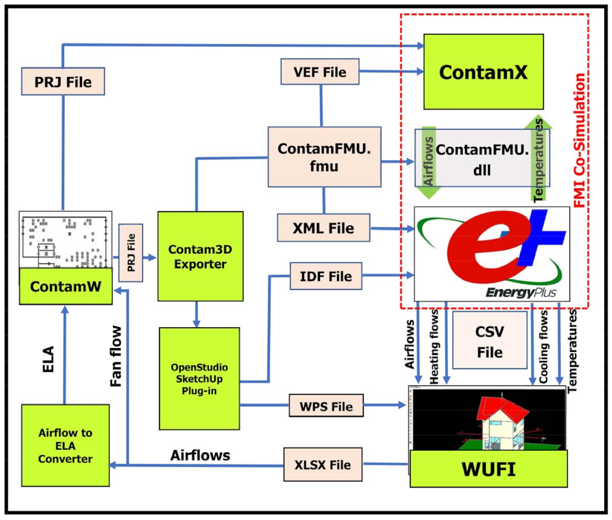
As shown in Figure 1, the interconnection and consequently integrations between each of the sub-models of EnergyPlus, CONTAM, and WUFI have been applied subject to the exchange of common control variables. The most important of these common control variables are indoor air temperatures and different types of airflows in the form of infiltration, natural, and mechanical ventilation. The three sub-models have been integrated into three phases according to Figure 1. In this interrelationship, common control variables are exchanged in a conversion loop between the three sub-models.

In the first phase, the coupling mechanism between EnergyPlus and CONTAM is performed based on the co-simulation method. This method was developed by Dols et al. [12]. The co-simulation method based on the standard functional mock-up interface provides the link between EnergyPlus and CONTAM [35]. The functional mock-up interface (FMI) standard is a tool-independent standard that supports exchange data and co-simulation of dynamic models [36]. The CONTAM model consists of two separate programs: (1) ContamW and (2) ContamX [10]. The ContamW runs as a graphic user interface and can be used to define the case of the building and also to view the simulated results. The ContamX, however, simulates and calculates indoor air quality measures. The input data related to the description of the building case study is saved as a project (PRJ) file in ContamW and can also be read in ContamW and ContamX. For co-simulation, the CONTAM model must first be implemented in the FMI standard. This model is implemented by exporting the CONTAM model into a functional mockup unit (FMU). The created FMU is called ContamFMU.fmu, which is a compressed zip file and can then be imported into EnergyPlus for co-simulation. The program that exports the CONTAM model to ContamFMU.fmu is called the CONTAM3DExporter tool which was developed by the National Institute of Standards and Technology (NIST) [37].

The CONTAM3DExporter tool converts the PRJ file created by ContamW into two files as shown in Figure 1. These two files are (1) input data file (IDF file) and (2) ContamFMU.fmu. The IDF file contains information about geometry, airflow infiltration, inter-zone airflow, and HVAC system airflows. Finally, this IDF file is provided to EnergyPlus. ContamFMU.fmu includes packages of compressed zipped files for controlling and exchanging common variables between EnergyPlus and CONTAM. The components of this package include XML file, VEF file, ContamFMU.dll (XML: extensible markup language, VEF: variable exchange file and dll: dynamic link library), and other files required in co-simulation. The XML file is exchanged with EnergyPlus and provides data on zone infiltration, inter-zone airflows, and control values of airflow ventilation. The VEF file is exchanged with ContamX and provides data on zone temperature, ventilation system airflows, outdoor airflow fractions, exhaust fan airflow, outdoor environment data, and output variables. Additionally, the ContamFMU.dll acts as a control file in exchanging temperature and airflow control variables along with other required information between EnergyPlus and ContamX. The temperatures and airflow control variables are exchanged between EnergyPlus and ContamX as shown in Figure 1 using ContamFMU.dll. This exchange leads to the integration of these two sub-models and the creation of coupled EnergyPlus–CONTAM [34].

In the second phase, the simulated variables resulted from the co-simulation in the previous phase are used as WUFI input data. Thus, the interconnection is made between the coupled EnergyPlus-CONTAM with WUFI. This mechanism is based on the replacement of simulated variables of coupled EnergyPlus-CONTAM with input data of WUFI. In this replacement control variables, airflows, temperature, heating, and cooling flows are exchanged as CSV files (CSV: comma-separated values) as shown in Figure 1. The simulated paths and ducts airflows in coupled EnergyPlus-CONTAM are replaced separately with input data of natural, mechanical, and interzone airflows in WUFI. The simulated heating and cooling temperatures in coupled EnergyPlus-CONTAM are replaced with input data of maximum and minimum temperatures in WUFI. Finally, the simulated space heating and cooling energy consumptions per hour in coupled EnergyPlus-CONTAM are also replaced by input data of heating and cooling space capacities in WUFI.

Integration of the developed model is completed by performing the third phase. This phase consists of two parts. In the first part, the airflows control variables simulated in WUFI as shown in Figure 1 are used as input data for flow rates of exhaust fan and leakage area. The simulated control variables related to the natural and mechanical ventilation in WUFI in the form of an XLSX file, as shown in Figure 1, are replaced by the input data of ELA (effective leakage area) and fan flow rate in ContamW, respectively. The simulated natural ventilation of WUFI is replaced with ELA input data in ContamW by using an Excel converter (airflow to effective leakage area converter tool).

The airflow to ELA converter operates on the basis of Equations (1)–(3) [18,38,39].

$$ACH=\frac{\dot{m}}{V_{net}}$$

(1)

$$NL\approx ACH$$

(2)

$$NL=1000·\frac{ELA}{A_f}·{\left(\frac{H}{2.5}\right)}^{0.3}$$

(3)

where $ACH$ for air change per hour (h⁻¹), $\dot{m}$ for volumetric airflow rate (m³/h), $V_{net}$ for building net volume (m³), $NL$ for normalized leakage, ELA for effective leakage area, $A_f$ for floor area (m²) and $H$ for building height (m) are considered (for more details regarding airflow element models and effective leakage area calculation conditions values in ContamW, see [18]).

In the next step, the geometry data simulated by ContamW is converted from the PRJ file to an IDF file with the help of CONTAM3DExporter. The IDF file can be viewed and edited by the importer of the OpenStudio SketchUp Plug-in extension and the details of this geometry can also be controlled and modified [40]. The geometry modified file can be exported from SketchUp into WUFI by the WUFI SketchUp’s Plug-in as an extension in SketchUp. The format of this imported file is WPS (WUFI Passive-SketchUp) for geometry files. In this procedure, the simulated modified geometry data is used as input geometry data in WUFI.

The exchange of both airflows and geometry control variables as shown in Figure 1 between WUFI and CONTAM completes the interconnection process in the final step. Exchange of common control variables airflows, temperatures, heating and cooling flows, geometry data, and other involved variables, leads to integration between sub-models of EnergyPlus, CONTAM, and WUFI dynamically resulting in simulating the energy, indoor air quality, and moisture for whole-building performance.

2.2. Governing Equations

The equations for the integrated model are the combination of the energy, moisture, and contaminant flow balances according to Equations (4)–(6), respectively.

$$\frac{d{E}_{heat,i}}{dt}={{\displaystyle \sum }}_k{\dot{E}}_{component,k}^{opaque}+{{\displaystyle \sum }}_k{\dot{E}}_{component,k}^{transparent}+{\dot{E}}_{solar}+{\dot{E}}_{internal}+{\dot{E}}_{nat-infiltration}+{\dot{E}}_{mech-ventilation}$$

(4)

$$\frac{d{w}_{moist,i}}{dt}={{\displaystyle \sum }}_k{\dot{w}}_{component,k}+{\dot{w}}_{indoor}+{\dot{w}}_{nat-infiltration}+{\dot{w}}_{mech-ventilation}$$

(5)

$$\frac{d{m}_{cont,i}^{\alpha }}{dt}={\displaystyle \sum }_j{\dot{m}}_{air-inwar{d}_{\left(j,i\right)}}·\left(1-{\eta }_{j,·i}^{\alpha }\right)·C_j^{\alpha }+G_i^{\alpha }+m_{ai{r}_i}·{\displaystyle \sum }_{\beta }{K}_i{}^{\alpha ,\beta }·C_i^{\beta }-{\displaystyle \sum }_j{\dot{m}}_{air-outwar{d}_{\left(i,j\right)}}·C_i^{\alpha }-R_i^{\alpha }·C_i^{\alpha }$$

(6)

In Equations (4)–(6), $\frac{d{E}_{heat,i}}{dt}$ as heat flow rate in the zone i (room) (W), $\frac{d{w}_{moist,i}}{dt}$ as moisture flow rate of the zone i (kg/s) and $\frac{d{m}_{cont,i}^{\alpha }}{dt}$ as contaminant of α flow rate in the zone i (kg/s) have been calculated [41,42,43].

In the integrated model, all three equations related to the balances of energy, moisture, and contaminant flows are connected to each other by exchanging two types of common control variables. These two common control variables are airflows and temperatures. The airflows are created by air exchange as a result of infiltration, natural and mechanical ventilation between the interior and the exterior air of the building. Air exchange is associated with changes in the air temperatures of zones.

The airflows of natural ventilation and infiltration (${\dot{m}}_{nat-infiltration}$), and supply mechanical ventilation (${\dot{m}}_{supply}$) are connected to each other via the equations of energy and moisture flow balances, according to Equations (7)–(15). The total airflow according to Equation (16) is equal to the sum of ${\dot{m}}_{nat-infiltration}$ and ${\dot{m}}_{supply}$. According to Equation (17), this total airflow can replace the airflows of ${\dot{m}}_{air-outwar{d}_{\left(i,j\right)}}$ and ${\dot{m}}_{air-inwar{d}_{\left(j,i\right)}}$ in the contaminant flow balance. Thus, the airflows control variables are exchanged between all three equations of energy, moisture, and contaminant flows balances. Equations (7)–(9) relate to the calculation of energy flows due to natural ventilation, infiltration, and mechanical ventilation as part of the energy balance equation.

$${\dot{E}}_{nat-infiltration}={\dot{m}}_{nat-infiltration}·\left(h_i-h_o\right)$$

(7)

$$h_i-h_o=\left(1006+x_o·1840\right)·\left(T_i-T_o\right)$$

(8)

Convective heat flow from building mechanical ventilation systems (${\dot{E}}_{mech-ventilation}$) is calculated by Equation (9).

$${\dot{E}}_{mech-ventilation}={\dot{m}}_{supply}·\left(h_i-h_o\right)·\left(1-{\eta }_{HR}\right)$$

(9)

In Equations (10)–(15), the moisture flows due to natural ventilation, infiltration, and mechanical ventilation as part of the moisture balance equation have been calculated.

$${\dot{w}}_{nat-Infiltration}={\dot{m}}_{nat-Infiltration}·\left(x_o-x_i\right)$$

(10)

$$x_o=0.622·\frac{P_{p_o}}{P_b-P_{p_o}}$$

(11)

$$x_i=0.622·\frac{P_{p_i}}{P_b-P_{p_i}}$$

(12)

$$P_{p_o}=\phi ·P_{s_o}\left(T_o\right)$$

(13)

$$P_{p_i}=\phi ·P_{s_i}\left(T_i\right)$$

(14)

In Equations (14)–(18), $x_i$, $P_{p_o}$, $P_{p_i}$, $P_b$, $\phi$, $P_{s_o}$ and $P_{s_i}$ are moisture content of inner air (kg/kg), water vapor partial pressure of outer air (Pa), water vapor partial pressure of inner air (Pa), barometric pressure (Pa), relative humidity, saturated vapor pressure depending on outer air temperature (Pa), and saturated vapor pressure depending on inner air temperature (Pa), respectively.

$${\dot{w}}_{mech-ventilation}={\dot{m}}_{supply}·\left(x_o-x_i\right)·\left(1-{\eta }_{MR}\right)$$

(15)

In Equation (16), the total airflow of ith zone (${\dot{m}}_{{\left(air-total\right)}_i}$), is resulted by airflow rates of natural ventilation and infiltration (${\dot{m}}_{nat-infiltration}$) plus supply mechanical ventilation (${\dot{m}}_{supply})$.

$${\dot{m}}_{{\left(air-total\right)}_i}={\dot{m}}_{nat-infiltration}+{\dot{m}}_{supply}$$

(16)

$${\dot{m}}_{air-inwar{d}_{total}}={\dot{m}}_{air-outwar{d}_{total}}={\dot{m}}_{{\left(air-total\right)}_i}$$

(17)

According to Equation (17), this total airflow of ith zone replaces the total of outward and inward airflows (${\dot{m}}_{air-outwar{d}_{total}},·{\dot{m}}_{air-inwar{d}_{total}}$) used in the contaminant balance equation. In Equation (18), the total airflow of ith zone (${\dot{m}}_{{\left(air-total\right)}_i}$) depends on the density variable of the room air of ith zone (${\rho }_i$). According to Equation (19), this density depends on the densities for dry air (${\rho }_{a,i}$) and water vapor (${\rho }_{w,i}$) of ith zone. The densities of dry air (${\rho }_{a,i}$) and water vapor (${\rho }_{w,i}$) of ith zone depend on the absolute inner air temperature of ith zone (${\theta }_i$) in Equations (20) and (21), respectively, and finally the absolute inner air temperature of ith zone (${\theta }_i$) depends on the inner air temperature ($T_i$) of ith zone in Equation (22).

Based on this, it can be concluded that the total airflow of the ith zone depends on the inner air temperature of the ith zone. Therefore, the mechanism of exchange of the inner air temperature of the ith zone between all three equations of energy, moisture, and contaminant balances can prove the interdependency of total airflow to inner air temperature based on Equations (18)–(22). Due to the dependence of total airflow on inner air temperature, it can be concluded that temperatures are exchanged simultaneously with the exchange of airflows control variables.

$${\dot{m}}_{{\left(air-total\right)}_i}={\dot{V}}_{{\left(air-total\right)}_i}·{\rho }_i$$

(18)

$${\rho }_i={\rho }_{a,i}+{\rho }_{w,i}$$

(19)

$${\rho }_{a,i}=\frac{P_b-P_{p_i}}{R_a·{\theta }_i}$$

(20)

$${\rho }_{w,i}=\frac{P_b-P_{p_i}}{R_w·{\theta }_i}$$

(21)

$${\theta }_i=273.15+T_i$$

(22)

In Equations (18)–(22), ${\dot{m}}_{{\left(air-total\right)}_i}$, ${\dot{V}}_{{\left(air-total\right)}_i}$, ${\rho }_i$, ${\rho }_{a,i}$, ${\rho }_{w,i}$, $R_a$, $R_w$ and ${\theta }_i$ are total airflow of ith zone (kg/s), total volumetric airflow of ith zone (m³/s), density for the room air of ith zone (kg/m³), density for dry air of ith zone (kg/m³), density for water vapor of ith zone (kg/m³), gas constant of dry air (=287.05 J/kgK), gas constant water vapor (=461.495 J/kgK), and absolute inner air temperature of ith zone (K).

The dependence of energy flow on temperatures can be proved based on Equations (7)–(9). In these equations, the relationships between specific enthalpy of the inner air ($h_i$) and specific enthalpy of the outer air ($h_o$) with the outer air temperature ($T_o$) and the inner air temperature ($T_i$) of ith zone, respectively, are presented. The dependence of moisture flow on temperatures can be proved based on Equations (10)–(15). In these equations, the relationships between moisture content of outer air ($x_o$) and moisture content inner air ($x_i$) with outer air temperature ($T_o$) and inner air temperature ($T_i$) of ith zone, respectively, are presented. The exchange of total airflow and inner air temperatures between the equations of energy, moisture, and contaminant flows balances as common variables lead to the combination potentials of energy, moisture, and indoor air quality models.

2.3. The Case Study Description

The case study is a three-story house. This case has three levels: basement, main floor, and bedrooms floor. The basement includes a utility room, exercise room, parking, and staircase with an area of 35.67 m² and a volume of 107.01 m³. The main level includes the living room, kitchen, washroom, and staircases with an area of 38.12 m² and a volume of 114.36 m³. 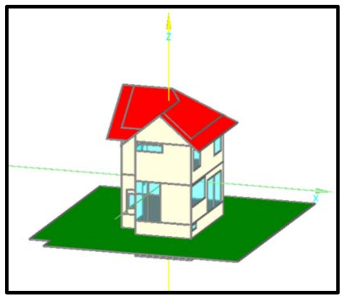The bedroom level includes three bedrooms, two bathrooms, a hall, and staircases with an area of 35.93 m² and a volume of 107.79 m³. The floor plans and a 3D view of the three-story house are shown in Figure 2 and Figure 3, respectively. Figure 2, created by WUFI, shows the position of all three levels of the basement, main and bedrooms, as well as the configuration of each of the components of exterior walls, roof, windows, and other openings in a 3D view in order to introduce the style of this type of residential three-story house. Figure 3, designed by CONTAM, shows the floor plans of the three-story-house case study to locate the levels of the basement (utility room, exercise room, parking, and staircase), main (living room, kitchen, washroom, and staircases) and bedrooms (three bedrooms, two bathrooms, hall, and staircases), with configurations of zones, AHS (air-handling system), source and sinks of contaminants, walls, and airflow paths.

A total floor area of 109.72 m², net volume of 329.16 m³, floor-to-ceiling height of 2.7 m, orientation of 0–180°and the window to the wall ratio of S, E, N, 40% have been assumed as geometry for the case study. The envelope effective leakage area (ELA) of this case study is considered at a pressure of 4 Pa, exponent of 0.65, discharge coefficient of 1 for the airtight and leaky cases of 0.04 m² and 0.3 m² [39], respectively. The exhaust fan with the flow rates of 24 L/s is operated in an on or off position. The number of zones and envelope airflow paths are 15 and 42, respectively. Envelope airflow paths represent doors, windows, cracks, and exhausts. A simple recirculating air handling system (AHS) with a total volumetric airflow of 0.35 m³/s is used in this house. The maximum space heating and cooling loads for this case study are 18.16 kW and 5.2 kW for Montreal, respectively, 15.10 kW and 5.2 kW for Vancouver, respectively, 10.59 kW and 7 kW for Miami, respectively, [44,45]. Moreover, the maximum airflow required to provide space heating/cooling loads in Montreal, Vancouver, and Miami are 0.4 m³/s, 0.365 m³/s, and 0.377 m³/s [46]. A design condition zone temperature of 20 °C has been defined.

The occupants of the case study include an adult male, an adult female, and also three children of ages 4, 10, and 13 years. The indoor sources of CO₂ in this study are the respiration of the occupants. Indoor CO₂ generation rates of 11 mg/s and 9.8 mg/s in awake and 6.6 mg/s and 6.2 mg/s in sleeping, have been considered for the adult male and female, respectively [47]. Indoor CO₂ generation rates of 3.8 mg/s, 6.8 mg/s, and 8.6 mg/s in awake and 2.3 mg/s, 4.1 mg/s, and 5.2 mg/s in sleeping, have been considered for the children of ages 4, 10, and 13 years, respectively [47]. The air filter with a MERV (minimum efficiency reporting value) rating of 4 with the supply of AHS ventilation has been used.

Heat transfer coefficient (U-value) or thermal resistance (RSI: R-value system international) for assemblies used in case study’s components of the ground floor, below-grade walls, above-grade walls, intermediate floor ceilings, roof, external doors, and interior walls are determined based on the climate zones categorized in ASHRAE Standard 90.1. The cities of Montreal, Vancouver and Miami are categorized into ASHRAE climate zones of 6-A, 5-A, and 1-A, respectively. Climate zones of 6-A, 5-A, and 1-A are defined as cold-humid, moderate-humid, and warm-humid in ASHRAE Standard 90.1. Based on this, the maximum acceptable U-value or minimum acceptable RSI in ASHRAE Standard 90.1 is considered as the assemblies’ U-value or RSI input data criteria. Window types of the case study have also been selected based on ASHRAE criteria from the WUFI database. In this database, reflected double-glazed windows with a U-value of 2.730 W/m²·K and frame factor of 0.7 for Montreal and Vancouver as well as the window type of reflective aluminum frame-fixed with U-value of 3.610 W/m²·K and frame factor of 0.7 for Miami are assumed.

In Montreal, for ground floor with RSI of 13.221 m² K/W, for below-grade walls with 5.445 RSI of m² K/W, for above-grade walls with RSI of 7.070 m² K/W, for intermediate floor ceilings with RSI of 6.801 m² K/W, for roof with RSI of 10.488 m² K/W, for reflected double-glazed windows with RSI of 0.366 m² K/W, for external doors with RSI of 0.350 m² K/W and for interior walls with RSI of 1.2 m² K/W have been assumed [45]. In Vancouver, for ground floor with RSI of 10.671 m² K/W, for below-grade walls with RSI of 3.695 m² K/W, for above-grade walls with RSI of 7.070 m² K/W, for intermediate floor ceilings with RSI of 6.801 m² K/W, for roof with RSI of 10.488 m² K/W, for reflected double-glazed windows with RSI of 0.366 m² K/W, for external doors with RSI of 0.350 m² K/W and for interior walls with RSI of 1.2 m² K/W have been considered [45]. In Miami, for ground floor with RSI of 5.241 m² K/W, for below-grade walls with RSI of 0.695 m² K/W, for above-grade walls with RSI of 4.445 m² K/W, for intermediate floor ceilings with RSI of 0.651 m² K/W, for roof with RSI of 4.678 m² K/W, for reflective aluminum frame-fixed windows with RSI of 0.277 m² K/W, for external doors with RSI of 0.350 m² K/W and for interior walls with RSI of 1.2 m² K/W have been chosen [45].

The materials of XPS (extruded polystyrene) surface skin, XPS Core, XPS surface skin, concrete w/c (water-cement-ratio) of 0.5, PVC roof membrane, EPS (expanded polystyrene, except for Miami), and gypsum-fiberboard have been used from outside to inside for ground floor. The materials of mineral plaster, oriented strand board, wood-fiberboard, EPS (except for Miami), polyethylene membrane, chipboard, and gypsum board have been assumed from outside to inside for below-grade walls. The materials of mineral plaster, oriented strand board, wood-fiberboard, EPS, polyethylene membrane, chipboard, and gypsum board have been selected from outside to inside for above-grade walls. The materials of oak-radial, air layer, EPS (except for Miami), softwood, and gypsum board have been considered from outside to inside for intermediate floor ceilings. The materials of 60-min building paper, mineral insulation board, softwood, vapor retarder, air layer, wood-fiber insulation board, polyethylene membrane, and softwood have been assumed from outside to inside for the roof. The wall-to-roof and wall-to-floor thermal bridges are 0.03 W/m·K, 0.04 W/m·K, respectively.

The data assumptions of infiltration, ventilation, envelope, geometry, occupants, and thermal bridges have been applied as input data for EneegyPlus. The input data of envelope leakage area, number of envelope paths, flow rate of the exhaust fan number of zones, indoor contaminant source elements, concentrations of outdoor contaminants, contaminants types, contaminants generation rates, and air-handling systems capacities are considered for the CONTAM model. The input parameters of geometry, internal load category, component assembly U-value, design conditions temperature, HVAC load and capacities, infiltration, and ventilation rates are used for the WUFI model. The input data and formats for EnergyPlus is EPW (EnergyPlus weather file) [48]. CONTAM can use the weather data files by using CONTAM Weather File Creator to convert the EPW file to a WTH (weather) [49]. In WUFI, the weather data files have been selected from the weather database. Finally, all input data for EnegyPlus, CONTAM, and WUFI models are used as input data for the integrated model for comparison and analyzing the simulated results (for more details see [18]).

2.4. Developed Integrated Model Verification

The present integrated model has been verified based on paired sample t-test method by using the SPSS tool [50] as the statistical method. This method was previously used for the verification of energy models [51,52,53]. The reasons for choosing the paired sample t-test method to verify the accuracy of the present integrated model are: (a) it is simple and valid as a statistical method for analyzing the differences between actual and simulated data, and (b) this method is quite accurate where the differences between the actual and simulated data are tested in two steps based on statistically reliable criteria. These two steps include (1) paired samples difference and (2) paired samples correlation.

Briefly, in paired samples difference method, the difference between the actual and simulated data samples was tested. When the standard deviation differences between the actual and simulated data are greater than half of the mean difference and also the significance level is greater than 0.05, then it is concluded that there is no significant difference between the actual and simulated data. When this step is confirmed, the second step for paired sample correlation is then performed for further testing.

In the paired samples correlation method, the correlations between the actual and simulated samples are tested. When the correlation coefficient between the actual and simulated data is greater than 0.5 and the significance level is less than 0.05, then there is no significant difference between the actual and simulated data. When the second stage of the test is also confirmed, it can be concluded that the actual and simulated data are very similar based on statistical criteria.

In this research, the values of daily space heating energy consumption, daily indoor CO₂ concentration, and hourly relative humidity (RH) are selected as energy, indoor air quality, and moisture data, respectively.

The actual and simulated values of these data for the three-story house case of leaky fans on in Montreal are shown in

Table 1. Daily space heating energy consumption data of the 15th day of the months in 2020 for cases of leaky fans on in Montreal.

Data (kWh)	Month
	January	February	March	April	May	June	July	August	September	October	November	December
Actual	14.48	23.24	45.84	47.92	43.90	9.88	1.08	0.00	17.24	43.40	46.60	45.84
Simulated	14.82	23.30	45.49	47.70	43.06	9.56	1.44	0.00	17.59	43.55	46.44	45.67

,

Table 2. Daily indoor CO₂ concentration data of the 15th day of the months in 2020 for cases of leaky fans on in Montreal.

Data ((kg/kg) × 10−4)	Month
	January	February	March	April	May	June	July	August	September	October	November	December
Actual	8.32	8.60	8.69	8.47	8.76	8.77	8.50	8.77	8.72	8.42	8.63	8.56
Simulated	8.01	8.55	8.72	8.27	8.85	8.89	8.36	8.91	8.84	8.27	8.74	8.68

and

Table 3. Hourly relative humidity (RH) data of the 15th day of the months in 2020 for cases of leaky fans on in Montreal.

Data (%)	Month
	January	February	March	April	May	June	July	August	September	October	November	December
Actual	58.71	66.88	63.02	57.12	53.57	68.86	64.62	61.37	74.23	68.74	70.10	68.29
Simulated	52.50	68.98	61.09	49.14	40.78	70.12	61.33	55.08	81.33	70.51	72.50	68.95

. Table 1 presents daily space heating energy consumption data for the 15th day of each month of the year 2020 for the case of leaky fans on in Montreal. The simulated data is calculated using the integrated model and the actual data is measured by the plug-in energy monitor.

Table 2 shows the daily indoor CO₂ concentration data for the case of leaky fans on in Montreal for the 15th day of each month for 2020. The simulated data is calculated by the integrated model and the actual data is measured by the CO₂ meter monitor.

The hourly relative humidity (RH) data for the case of leaky fans on in Montreal for the 15th day of each month for 2020. In this table, the values of the simulated data are calculated by the integrated model and the actual values are measured by the humidity meter monitor.

The results of paired samples differences and paired sample correlation analysis for actual and simulated data for the case of leaky fans on in Montreal are shown in

Table 4. Paired sample difference t-test results between actual and simulated data for space heating energy consumption, indoor CO₂ concentration, and indoor relative humidity (RH) in 2020 for cases of leaky fans on in Montreal.

Actual vs. Simulated Data		Paired Differences
		Mean	Standard. Deviation	Standard. Error Mean	95% Confidence Interval of the Difference		t-Value	df	Significance (Two-Tailed)
					Lower	Upper
1	Daily space heating energy consumption (kWh)	0.06667	0.35341	0.10202	−0.15788	0.29121	0.653	11	0.527
2	Daily indoor CO2 concentration ((kg/kg) × 10−4)	0.01000	0.15474	0.04467	−0.08832	0.10832	0.224	11	0.827
3	Hourly Indoor relative humidity (%)	1.93333	5.56633	1.60686	−1.60334	5.47001	1.203	11	0.254

and

Table 5. Paired sample correlation t-test results between actual and simulated data for space heating energy consumption, indoor CO₂ concentration, and indoor relative humidity (RH) in 2020 for cases of leaky fans on in Montreal.

Actual vs. Simulated Data		Measurers
		N	Correlation	Level of Significance
1	Space heating energy consumption (kWh)	12	1.000	0.000
2	Indoor CO2 concentration ((kg/kg) × 10−4)	12	0.973	0.000
3	Indoor relative humidity (%)	12	0.995	0.000

, respectively.

Table 4 reveals that the standard deviation difference between actual and simulated data for daily space heating energy consumption, daily indoor CO₂ concentration, and hourly relative humidity (RH) are 0.35341, 0.15474, and 5.56633, respectively (being > half mean difference) with the significance level of 0.527, 0.827 and 0.254, respectively (being > 0.05). As such, there are no significant differences between actual and simulated data for space heating energy consumption, indoor CO₂ concentration, and relative humidity (RH).

Table 5 shows that the correlation coefficients for actual and simulated data of space heating energy consumption, indoor CO₂ concentration and indoor relative humidity (RH) are 1.000, 0.973, and 0.995, respectively (being > 0.5) with a significance level of <0.05. Thus, the actual and simulated data are in good agreement.

According to the results of using the paired sample t-test method for evaluating the differences between actual and simulated data, the integrated model showed a high accuracy.

3. Results

The effect of the accuracy of the results simulated by the integrated model compared to the single models is presented in this section. Four scenarios are defined for a case of a three-story house.

For a case of a three-story house subjected to three different climatic zones of Montreal, Vancouver, and Miami, the scenarios that were chosen to analyze the accuracy of the integrated model compared to single models are based on 4 common features: (1) reducing energy consumption with reducing indoor air quality, (2) reducing energy consumption with increasing indoor air quality, (3) investigate the moisture performance due to reducing indoor air quality, and (4) investigate the moisture performance due to increasing indoor air quality. These four scenarios are called in this study as: (1) airtight fan off, (2) airtight fan on, (3) leaky fan off, and (4) leaky fan on. Additionally, by choosing these four scenarios, the accuracy of the integrated model in determining the optimal scenarios in each of energy performance, indoor air quality, and moisture performance can be evaluated more simply and realistically compared to single models.

The measures of space heating/cooling energy consumptions, indoor CO₂ concentration, and relative humidity (RH) for all four scenarios are simulated in the first phase by single models of EnergyPlus, CONTAM, and WUFI, respectively. In the second phase, all measures of space heating/cooling energy consumptions, indoor CO₂ concentration, and relative humidity (RH) are simulated by the integrated model.

The single models with the integrated model scenarios are compared by using the percentage differences of the simulated results with the acceptable level of ASHRAE Standards in different climates of Montreal, Vancouver, and Miami for each scenario.

3.1. Results of the Single Model of EnergyPlus

In this research, the simulated hourly space heating/cooling energy consumptions obtained with EnergyPlus are considered as energy performance measures for different scenarios of a three-story house. The energy performance measure is presented in these results by calculation of the percentage difference between the simulated hourly space heating/cooling energy consumptions and the acceptable ASHRAE Standard 90.1 level [45]. The obtained results for all four scenarios of airtight fans off, airtight fan on, leaky fan off, and leaky fan on are shown in Figure 4a–c. These results are compared for three different climatic conditions of Montreal, Vancouver, and Miami.

3.2. Results of the Single Model of CONTAM

The results of simulated daily indoor CO₂ concentration are obtained by CONTAM as indoor air quality performance for different three-story house case scenarios. The indoor air quality measure is presented in the results based on the calculation of the percentage difference between the simulated daily indoor CO₂ concentrations and the ASHRAE Standard 62.1 level [54]. The results for each of the four scenarios of airtight fans off, airtight fan on, leaky fan off, and leaky fan on are shown in Figure 5a–c for three different climatic conditions of Montreal, Vancouver, and Miami.

3.3. Result of the Single Model of WUFI

The simulated hourly indoor relative humidity (RH) obtained by WUFI is considered as moisture performance for the three-story house case with different scenarios. This measure is presented as a result based on the calculation of the percentage difference between the simulated hourly indoor relative humidity (RH) levels and the ASHRAE Standard 160 level [54]. These results are shown for each of the scenarios (airtight fan off, airtight fan on, leaky fan off, and leaky fan on) in Figure 6a–c for three different climatic conditions of Montreal, Vancouver, and Miami.

3.4. Results of the Integrated Model

With the present integrated model, all three performances of energy, indoor air quality, and moisture are calculated simultaneously. The results of the integrated model are calculated based on the percentage differences between the levels of the simulated hourly space heating/cooling energy consumptions, simulated daily indoor CO₂ concentrations, and simulated hourly relative humidity (RH), with ASHRAE Standards 90.1, 62.1, and 160 levels, respectively these results are shown for each of the four scenarios of (1) airtight fan off, (2) airtight fan on, (3) leaky fan off and (4) leaky fan on in Figure 7, Figure 8 and Figure 9 for three climates of Montreal, Vancouver, and Miami.

4. Discussion

In this research study, an integrated model was developed to predict with high accuracy for building applications the energy, indoor air quality, and moisture performances, dynamically. The mechanism that was used to develop the integrated model is based on the exchange of airflows and temperatures control variables between EnergyPlus, CONTAM and WUFI sub-models. This model was developed in three phases. In the first phase, EnergyPlus, and CONTAM were coupled using a co-simulation method based on exchanging airflows and temperatures. The details and assessment of this method were presented in a previous study [34]. In the second phase, the CONTAM has been combined with WUFI. The mechanism of this combination is based on the exchange of simulated air flows, temperatures, heating, and cooling flow variables between CONTAM with WUFI input data [18]. In the final phase, which is the subject of this paper, the exchange of simulated WUFI airflows with the input data of CONTAM completes the EnergyPlus, CONTAM, and WUFI sub-models exchange control variables. The exchange of control variables between sub-models increases the integrated model accuracy. The integrated model’s accuracy was verified by using paired sample t-test method. Moreover, the predictions of the integrated model were compared with single models. These comparisons are applied to four different scenarios in a three-story house. The simulated results included measures of performance of energy, indoor air quality, and moisture.

In this study, the ASHRAE Standards 90.1, 62.1, and 160 were used as the standard criteria for calculating the performances of energy, indoor air quality, and moisture, respectively. Using the percentage difference method, the results of simulated hourly energy consumptions of space heating/cooling, daily indoor CO₂ concentrations, and hourly indoor relative humidity (RH) with acceptable levels of ASHRAE Standards 90.1, 62.1, and 160 are compared and their differences are calculated. This percentage difference for the results of all 4 scenarios is calculated by single models and integrated models. For different scenarios considered in this study, the simulation results of every single model and integrated model for Montreal, Vancouver, and Miami are presented separately in Figure 4, Figure 5, Figure 6, Figure 7, Figure 8 and Figure 9 and

Table 6. Energy performance analysis results by comparison of average percentage difference of simulated hourly space heating/cooling energy consumptions with ASHRAE Standard 90.1 level between EnergyPlus and the integrated model.

Energy Performance Analysis
Cities	Montreal		Vancouver		Miami
Models	EnergyPlus Model	Integrated Model	EnergyPlus Model	Integrated Model	EnergyPlus Model	Integrated Model
S1	−73.06%	−75.09%	−75.76%	−77.58%	−29.60%	−37.38%
S2	−40.97%	−46.85%	−54.17%	−56.35%	23.21%	12.09%
S3	−53.65%	−65.20%	−56.14%	−69.86%	−10.06%	−34.19%
S4	−26.01%	−40.12%	−35.14%	−48.65%	27.71%	8.25%

,

Table 7. IAQ performance analysis results by comparison of average percentage difference of simulated daily indoor CO₂ concentration with ASHRAE Standard 62.1 levels between CONTAM and the integrated model.

IAQ Performance Analysis
Cities	Montreal		Vancouver		Miami
Models	CONTAM Model	Integrated Model	CONTAM Model	Integrated Model	CONTAM Model	Integrated Model
S1	−79.17%	−79.32%	−79.08%	−79.09%	−79.63%	−79.63%
S2	−79.62%	−83.35%	−79.59%	−83.33%	−80.14%	−83.87%
S3	−80.95%	−80.26%	−80.66%	−79.85%	−80.29%	−79.68%
S4	−81.25%	−83.53%	−80.96%	−83.42%	−80.65%	−83.87%

and

Table 8. Moisture performance analysis results by comparison of average percentage difference of simulated hourly relative humidity (RH) with ASHRAE Standard 160 level between WUFI and the integrated model.

Moisture Performance Analysis
Cities	Montreal		Vancouver		Miami
Models	WUFI Model	Integrated Model	WUFI Model	Integrated Model	WUFI Model	Integrated Model
S1	−12.19%	14.92%	−8.36%	15.93%	12.01%	−4.64%
S2	−25.62%	14.17%	−19.58%	17.93%	9.21%	−0.99%
S3	−40.30%	15.99%	−31.44%	18.25%	0.99%	−4.15%
S4	−40.59%	15.15%	−31.71%	18.87%	0.90%	−1.25%

.

It is important to point out that the scenarios in which the simulated result values are less than the ASHRAE Standard level have a negative percentage difference. Moreover, the scenarios in which simulated results values are higher than the ASHRAE Standard level have a positive percentage difference. The results of the simulated results with the single models are compared with the present integrated model for performances of energy, indoor air quality, and moisture.

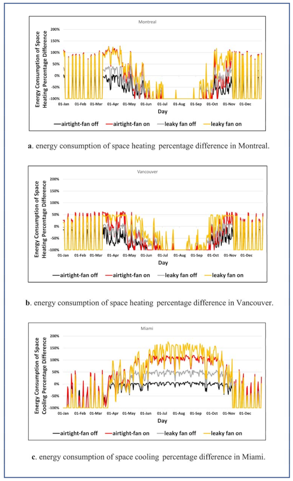
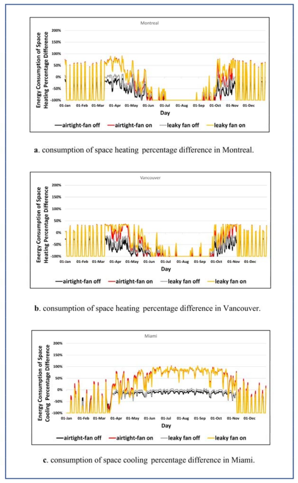
In Figure 4a–c, hourly energy consumptions (kWh) of space heating/cooling simulated by EnergyPlus, are compared with the acceptable power value (kW) of ASHRAE Standard 90.1, for scenarios 1, 2, 3, and 4, in Montreal, Vancouver, and Miami. The level that is acceptable by the ASHRAE Standard 90.1 is less than 1.72 kW for the building with a floor area of 109.72 m² [45]. Additionally, the simulated hourly space heating/cooling energy consumptions are compared with the acceptable level of ASHRAE Standard 90.1 (<1.72 kW), using the percentage difference method. The percentage difference is calculated by Equation (23) to compare the hourly space heating/cooling energy consumption results simulated by EnergyPlus with the level that is satisfactory by the ASHRAE Standard 90.1.

$$\begin{array}{c}\mathrm{Percentage}\mathrm{difference}\mathrm{of}\mathrm{energy}\mathrm{consumption}\left(\%\right)\hfill \\ =\frac{\mathrm{power}\mathrm{of}\mathrm{hourly}\mathrm{energy}\mathrm{consumption}\left(\frac{\mathrm{kWh}}{\mathrm{h}}\right)-\mathrm{ASHRAE}\mathrm{Standard}90.1\mathrm{level}\mathrm{of}1.72\mathrm{kW}}{\mathrm{ASHRAE}\mathrm{Standard}90.1\mathrm{level}\mathrm{of}1.72\mathrm{kW}}\times 100\hfill \end{array}$$

(23)

The usefulness of this method is, however, to present a dimensionless criterion as a percentage in order to compare the results of hourly space heating/cooling energy consumptions simulated by EnergyPlus for each of the scenarios with the level that is satisfactory by the ASHRAE Standard 90.1. These percentage differences are presented in four curves for each of the scenarios 1 to 4 for the entire days of 2020.

When the level of simulated hourly space heating/cooling energy consumption is more or less than the level that is satisfactory by the ASHRAE Standard 90.1, the resulted percentage difference values are positive or negative for different points of each of the four scenarios curves, respectively.

As shown in Figure 4a–c, in scenarios curves, the minimum values have the highest negative percentage difference compared to ASHRAE Standard 90.1 level (<1.72 kW) [45]. Therefore, these values have the highest performances. This percentage difference value is −100% in Montreal, Vancouver, Miami for scenarios 1 to 4. The percentage difference value of −100% means that since the maximum acceptable space heating/cooling energy consumption of ASHRAE Standard 90.1 per hour is 1.72 kW, then the value of hourly space heating/cooling energy consumption simulated by the EnergyPlus is zero kWh. When the value of zero kWh is calculated by Equation (23), the value of −100% has resulted.

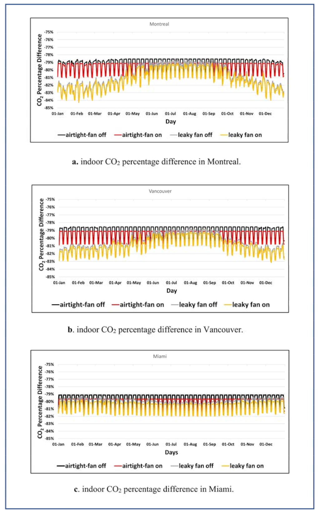
Figure 5a–c shows comparisons between daily indoor CO₂ concentrations (kg/kg) simulated by CONTAM and the level that is acceptable by the ASHRAE Standard 62.1, for scenarios 1 to 4, in Montreal, Vancouver, and Miami. The level that is acceptable by the ASHRAE Standard 62.1 for indoor CO₂ concentration is less than 52.32 × 10⁻⁴ kg/kg [54].

Equation (24) provides the percentage difference calculation relation for scenarios 1 to 4. Equation (24) is used in order to compare the results of daily indoor CO₂ concentrations simulated by CONTAM with an acceptable level of ASHRAE Standard 62.1.

$$\begin{array}{l}\mathrm{Percentage}\mathrm{difference}\mathrm{of}\mathrm{indoor}{\mathrm{CO}}_2\mathrm{concentration}\left(\%\right)\\ =\frac{{\mathrm{indoor}\mathrm{CO}}_2\mathrm{Concentration}\left(\frac{\mathrm{kg}}{\mathrm{kg}}\right)-\mathrm{ASHRAE}\mathrm{Standard}62.1\mathrm{level}\mathrm{of}52.32\times {10}^{-4}\frac{\mathrm{kg}}{\mathrm{kg}}}{\mathrm{ASHRAE}\mathrm{Standard}62.1\mathrm{level}\mathrm{of}52.32\times {10}^{-4}\frac{\mathrm{kg}}{\mathrm{kg}}}\times 100\end{array}$$

(24)

This method provides a dimensionless measure as a percentage to compare the results of daily indoor CO₂ concentrations, simulated by CONTAM for each of the scenarios with the acceptable level of ASHRAE Standard 62.1. These comparisons were performed in four curves of scenarios 1 to 4 for the days of 2020. If the level of simulated daily indoor CO₂ concentrations is more or less than the level that is acceptable by the ASHRAE Standard 62.1 criteria, then the values of percentage difference are positive or negative for different points of scenarios curves, respectively.

In scenarios curves, as shown in Figure 5a–c, the minimum values have the highest negative percentage difference compared to ASHRAE Standard 62.1 (indoor CO₂ < 52.32 × 10⁻⁴ kg/kg) [54]. So, these values have the highest performances. The percentage differences in the city of Montreal are calculated as the results values of −80.85% for scenario 1, −81.13% for scenario 2, −84.13% for scenario 3, and −84.30% for scenario 4. The percentage differences in the city of Vancouver are considered as the results values of −80.49% for scenario 1, −80.87% for scenario 2, −82.93% for scenario 3, and −83.15% for scenario 4. The percentage differences in Miami are calculated as the results values of −80.96% for scenario 1, −81.41% for scenario 2, −81.82% for scenario 3, and −81.98% for scenario 4.

Note that the percentage differences of all scenarios in CONTAM are less than −80%. These percentage differences values of less than −80% mean that since the maximum acceptable indoor CO₂ concentration according to ASHRAE Standard 62.1 is 52.32 × 10⁻⁴ kg/kg, so the daily indoor CO₂ concentrations simulated by CONATM are less than 51.90 × 10⁻⁴ kg/kg for all scenarios. As indicated above, the values of less than −80% are calculated by Equation (24) for all scenarios.

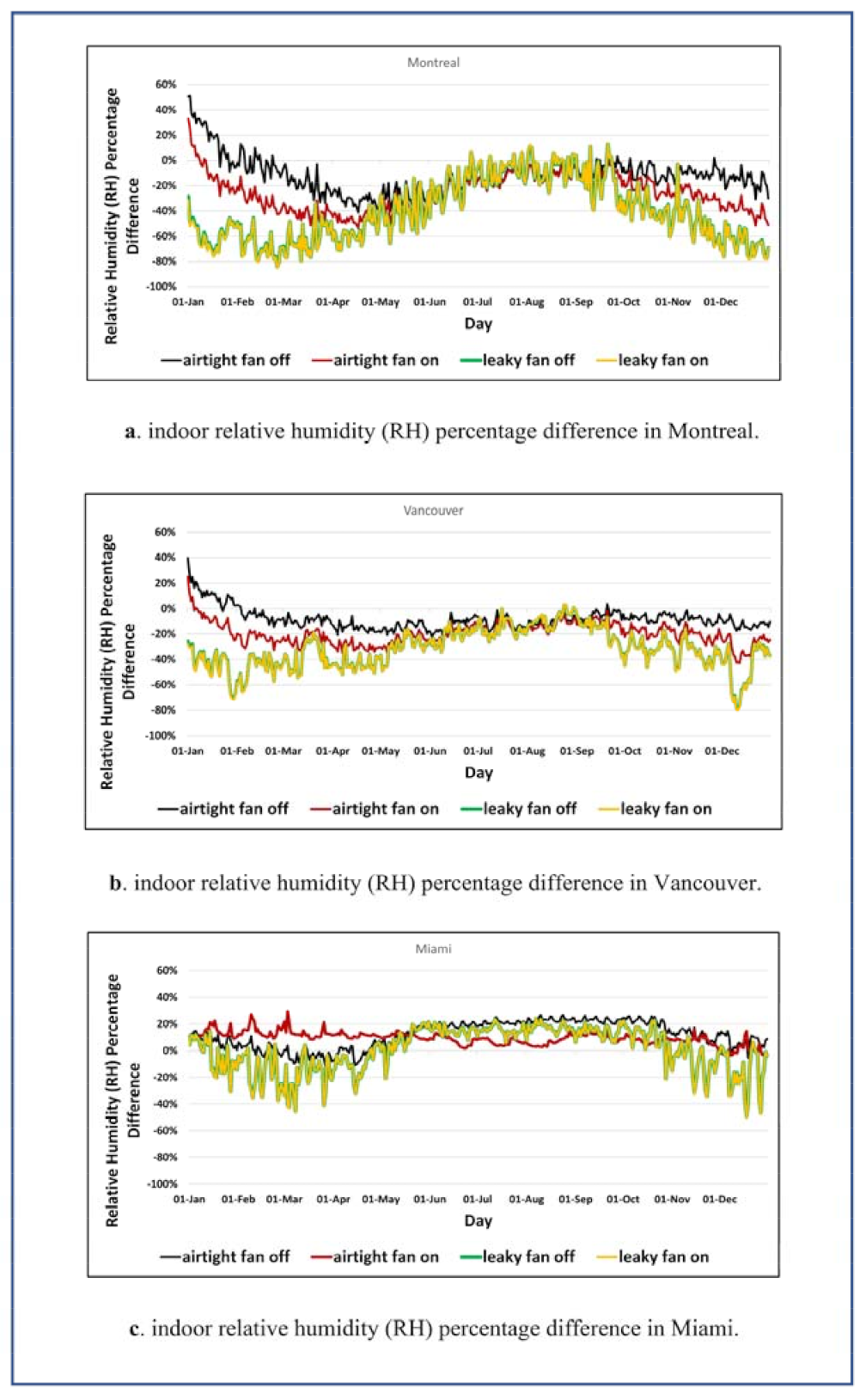
With WUFI according to Figure 6a–c, the simulated hourly indoor relative humidity (RH) is compared with the level that is satisfactory by the ASHRAE Standard 160, for scenarios 1 to 4, in Montreal, Vancouver, and Miami. The level that is acceptable by the ASHRAE Standard 160 for indoor relative humidity (RH) is less than 80% [54].

Finally, for the four scenarios considered in this study, the percentage difference is calculated by Equation (25) to compare the hourly indoor relative humidity (RH) results simulated by WUFI with the level that is acceptable by the ASHRAE Standard 160.

$$\begin{array}{l}\mathrm{Percentage}\mathrm{difference}\mathrm{of}\mathrm{indoor}\mathrm{relative}\mathrm{humidity}\left(\%\right)\\ =\frac{\mathrm{indoor}\mathrm{relative}\mathrm{humidity}\left(\%\right)-\mathrm{ASHRAE}\mathrm{Standard}160\mathrm{level}\mathrm{of}80\%}{\mathrm{ASHRAE}\mathrm{Standard}160\mathrm{level}\mathrm{of}80\%}\times 100\end{array}$$

(25)

The usefulness of this method is to create a dimensionless criterion as a percentage to compare the results of hourly indoor relative humidity (RH), simulated by WUFI for each of the scenarios with the level that is acceptable by the ASHRAE Standard 160. This percentage difference method has resulted in the four curves for four scenarios 1 to 4 for the days of 2020. When the level of simulated hourly indoor relative humidity (RH) is more or less than the level that is acceptable by the ASHRAE Standard 160, the values of percentage difference calculation are positive or negative for different points of scenarios curves, respectively.

According to Figure 6a–c, in scenarios curves, the minimum values have the highest negative percentage difference compared to ASHRAE Standard 160 level (indoor RH < 80%) [55]. Therefore, it is concluded that these values have the highest performances. The percentage differences in Montreal are considered as the results values of −41.29% for scenario 1, −53.60% for scenario 2, −84.18% for scenario 3, and −85.16% for scenario 4. The percentage differences in Vancouver are calculated as the results values of −22.10% for scenario 1, −43.06%, for scenario 2, −79.10% for scenario 3, and −80.13% for scenario 4. The percentage differences in Miami, are calculated as the results values of −11.83% for scenario 1, −3.57% for scenario 2, −49.26% for scenario 3, and −50.53% for scenario 4. Thus, the percentage differences of all scenarios are between −3.57% through −85.16%, which means that, since the maximum acceptable moisture content to minimize mold growth according to ASHRAE Standard 160 is 80%, so the hourly indoor relative humidity (RH), simulated by WUFI for all scenarios are between 79.97% through 79.31%. The percentage difference values between −3.57% through −85.16% for all scenarios in WUFI are calculated by Equation (25).

With the integrated model, the simulated hourly energy consumptions (kWh) of space heating/cooling, daily indoor CO₂ concentrations (kg/kg), and hourly indoor relative humidity (RH) (%) are compared with the levels that are acceptable by the ASHRAE Standards 90.1, 62.1 and 160, respectively, in cities of Montreal, Vancouver, and Miami for scenarios 1 to 4. Furthermore, the percentage difference method was used for comparing the simulated hourly energy consumptions of space heating/cooling, daily indoor CO₂ concentrations, and hourly indoor relative humidity (RH) with the levels that are acceptable by the ASHRAE Standards 90.1, 62.1, and 160, respectively.

For hourly energy consumptions (kWh) of space heating/cooling simulated by the integrated model, Figure 7a–c shows that in scenarios curves, the minimum values have the percentage difference compared to ASHRAE Standard 90.1. These values have the highest performances.

The percentage difference is calculated by Equation (23) to compare the hourly space heating/cooling energy consumption results simulated by the integrated model with the acceptable level of ASHRAE Standard 90.1. This percentage difference in Montreal, Vancouver, and Miami has resulted in a value of −100%. This means that since the maximum acceptable space heating/cooling energy consumption of ASHRAE Standard 90.1 per hour is 1.72 kW, so the value of hourly space heating/cooling energy consumption simulated by the integrated model is zero kWh. The value of −100% has resulted when the value of zero kWh is calculated by Equation (23).

For the simulated daily indoor CO₂ concentrations by the integrated model, Figure 8a–c, shows that in scenarios curves, the minimum values have the highest negative percentage difference compared to ASHRAE Standard 62.1. The values of these percentage differences have the highest performances. Equation (24) is used for the calculation of the percentage difference for comparing results of daily indoor CO₂ concentrations simulated by the integrated model with the level that is acceptable by the ASHRAE Standard 62.1. These percentage differences in Montreal are calculated as values of −81.18% for scenario 1, −84.17% for scenario 2, −82.86% for scenario 3, and −84.89% for scenario 4. The percentage differences in Vancouver are considered as the results values of −80.52% for scenario 1, −84.11% for scenario 2, −81.78% for scenario 3, and −84.30% for scenario 4. In Miami, this percentage difference is calculated as values of −80.96% for scenario 1, −84.65% for scenario 2, −81.10% for scenario 3, and −84.67% for scenario 4. The obtained percentage differences for all scenarios using the integrated model are less than −80%, which means that since the maximum acceptable indoor CO₂ concentration according to ASHRAE Standard 62.1 is 52.32 × 10⁻⁴ kg/kg, so the daily indoor CO₂ concentrations simulated by the integrated model are less than 51.90 × 10⁻⁴ kg/kg for all scenarios.

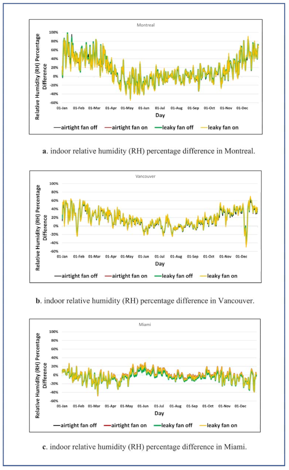
Additionally, for the simulated indoor relative humidity (RH) by the integrated model, Figure 9a–c shows that in scenarios curves, the minimum values have the highest negative percentage difference compared to ASHRAE Standard 160 and also have the highest performances.

The percentage difference in the integrated model is calculated by Equation (25) to compare the hourly indoor relative humidity (RH) results simulated by the integrated model with the level that is acceptable by the ASHRAE Standard 160. These percentage differences in Montreal are estimated as the results values of −46.35% for scenario 1, −52.44% for scenario 2, −50.37% for scenario 3, and −54.39% for scenario 4. These percentage differences in Vancouver are calculated as values of −36.92% for scenario 1, −47.67% for scenario 2, −43.55% for scenario 3, and −50.26% for scenario 4. The percentage differences in Miami are considered as results values of −42.63% for scenario 1, −47.88% for scenario 2, −44.75% for scenario 3, and −48.88% for scenario 4. The percentage difference of all scenarios in the integrated model is between −36.92% through −54.39%. These percentage difference values mean that, since the maximum acceptable moisture content to minimize mold growth according to ASHRAE Standard 160 is 80%, the hourly indoor relative humidity (RH), simulated by the integrated model for all scenarios, are between 79.70% through 79.56%.

Table 6, Table 7 and Table 8 show that the average performance of energy, indoor air quality, and moisture are compared for different scenarios between single and integrated models. The average performance calculation criterion is based on the average percentage difference of the simulated hourly space heating/cooling energy consumptions, daily indoor CO₂ concentration, and hourly indoor relative humidity (RH) with ASHRAE Standard 90.1, 62.1, and 160 levels.

As shown in Table 6 hourly energy consumptions of space heating/cooling, in Montreal, have been considered as the results average values of −73.06% for scenario 1, −40.97% for scenario 2, −53.65% for scenario 3, and −26.01% for scenario 4 by EnergyPlus and −75.09% for scenario 1, −46.85% for scenario 2, −65.20% for scenario 3, and −40.12% for scenario 4 by the integrated model, respectively.

The hourly energy consumptions of space heating/cooling in Vancouver (see Table 6), have been estimated as the results average values of −75.76% for scenario 1, −54.17% for scenario 2, −56.14% for scenario 3, and −35.14% for scenario 4 by EnergyPlus and −77.58% for scenario 1, −56.35% for scenario 2, −69.86% for scenario 3, and −48.65% for scenario 4 by the integrated model, respectively.

In Miami, according to Table 6, the hourly energy consumptions of space heating/cooling have been considered as the results average values of −29.60% for scenario 1, 23.21% for scenario 2, −10.06% for scenario 3, and 27.71% for scenario 4 by EnergyPlus and −37.38% for scenario 1, 12.09% for scenario 2, −34.19% for scenario 3, and 8.25% for scenario 4 by the integrated model, respectively.

According to Table 7, the daily indoor CO₂ concentration in Montreal has been calculated as the results average values of −79.17% for scenario 1, −79.62% for scenario 2, −80.95% for scenario 3, and −81.25% for scenario 4 by CONTAM, and −79.32% for scenario 1, −83.35% for scenario 2, −80.26% for scenario 3, and −83.53% for scenario 4 by the integrated model, respectively.

In Vancouver, the daily indoor CO₂ concentration (see Table 7) has been calculated as the results average values of −79.08% for scenario 1, −79.59% for scenario 2, −80.66% for scenario 3, and −80.96% scenario 4 by CONTAM, and −79.09% for scenario 1, −83.33% for scenario 2, −79.85% for scenario 3, and −83.42% for scenario 4 by the integrated model, respectively.

The daily indoor CO₂ concentration (see Table 7) in Miami has been considered as results average values of −79.63% for scenario 1, −80.14% for scenario 2, −80.29% for scenario 3, and 80.65% scenario 4 by CONTAM, and −79.63% scenario 1, −83.87% for scenario 2, −79.68% for scenario 3, and −83.87% for scenario 4 by the integrated model, respectively.

As shown in Table 8, the hourly indoor relative humidity (RH) in Montreal has been calculated as the results average values of −12.19% for scenario 1, −25.62% for scenario 2, −40.30% for scenario 3, and −40.59% for scenario 4 by WUFI, and 14.92% for scenario 1, 14.17% for scenario 2, 15.99% for scenario 3, and 15.15% for scenario 4 by the integrated model, respectively.

The hourly indoor relative humidity (RH) in Vancouver according to Table 8 has been estimated as the results average values of −8.36% for scenario 1, −19.58% for scenario 2, −31.44% for scenario 3, and −31.71% for scenario 4 by WUFI, and 15.93% for scenario 1, 17.93% for scenario 2, 18.25% for scenario 3, and 18.87% for scenario 4 by the integrated model, respectively.

In Miami, the hourly indoor relative humidity (RH), according to Table 8, has been considered as results average values of 12.01% for scenario 1, 9.21% for scenario 2, 0.99% for scenario 3, and 0.90% for scenario 4 by WUFI, and −4.64% for scenario 1, −0.99% for scenario 2, −4.15% for scenario 3, and −1.25% for scenario 4 by the integrated model, respectively.

For the results of the hourly space heating/cooling energy consumptions, by EnergyPlus and the integrated model, scenario 1 has resulted in the highest energy performance for different climatic conditions. With CONTAM to simulate the daily indoor CO₂ concentration, scenario 4 has resulted in the highest indoor air quality performance values in Montreal, Vancouver, and Miami, and for the integrated model scenario 4 in Montreal and Vancouver and both scenarios 2 and 4 in Miami have the highest indoor air quality performance value. For the simulated hourly indoor relative humidity measures simulated by WUFI, scenario 4 has resulted in the highest moisture performance values in Montreal, Vancouver, and Miami, and this measure simulated by the integrated model, for scenario 2 in Montreal, and scenario 1 in Vancouver and Miami have the highest indoor air quality performance. Given that the results of some scenarios with the highest performance values for indoor air quality and moisture measures for the cities of Vancouver, and Miami are different between single models and the present integrated model, it can be concluded that using the integrated model instead of single models seems necessary.

Considering that the reason for using the percentage difference method was to estimate the difference between the results of single models and the present integrated model with an acceptable level of ASHRAE Standards of 90.1, 62.1, and 160 by dimensionless percentage criteria, so this method makes it easier to compare simulated results. Therefore, it was possible to conduct comparisons for the average percentage difference of simulated results between the integrated model with single models as provided in Table 6, Table 7 and Table 8.

The percentage difference method was used to compare the results of scenarios 1, 2, 3, and 4 in Montreal, Vancouver, and Miami to choose the optimal scenario. When the percentage difference between the value of the result simulated by the integrated model or single models with an acceptable level of ASHRAE Standard is negative, the scenario with the highest difference is considered as the optimum scenario. Additionally, when the percentage difference is positive, the scenario with the lowest difference is selected as the optimal scenario. These optimal scenarios are chosen based on ASHRAE Standard 90.1, 62.1, and 160 criteria in terms of energy, indoor air quality and moisture, respectively, for Montreal, Vancouver, and Miami.

As shown in Table 6, Table 7 and Table 8, the average percentage difference of simulated results of the integrated model is different from single models for optimal scenarios. On the other hand, the accuracy of the integrated model for energy, indoor air quality, and moisture result samples have been verified by the paired sample t-test method presented in Table 4 and Table 5. The difference between the obtained results of a single method and the integrated method is due to the high accuracy of the present integrated model.

In summary, the reasons for the difference in the obtained results for the optimal scenarios simulated by single methods with the integrated method are:

• Scenario 1 is predicted as the optimal scenario for hourly energy consumptions of space heating/cooling in both EnergyPlus model and the integrated model methods, in Montreal, Vancouver, and Miami. The values of hourly energy consumptions of space heating/cooling for scenario 1 as the optimal scenario, by the integrated model method, are 2.77%, 2.40%, and 26.28% different from the EnergyPlus model method for Montreal, Vancouver, and Miami, respectively. The reason for this difference is that in the EnergyPlus model method, infiltration of 0.4 h⁻¹ and design air handling system airflow of 0.35 m³/s are defined as airflows input data by the user. In the integrated model, the airflow variables are corrected by the combination mechanism for EnergyPlus, CONTAM, and WUFI.
• Scenario 4 as an optimal scenario in terms of the daily indoor CO₂ concentration performance, through the integrated model method, 2.80% and 3.03% in Montreal and Vancouver are different from the CONTAM model method, respectively. The reason for this difference was because in the CONTAM model method, the effective leakage area of 0.3 m² and exhaust fan airflow of 24 L/s, as airflows input and junction temperature of 22.2 °C and default zone temperature of 20 °C as temperatures input data have been defined by the users. While the airflows and temperatures in the integrated model method have been corrected by the combination mechanism for EnergyPlus, CONTAM, and WUFI.
• In Miami, scenarios 2 and 4 for the daily indoor CO₂ concentration performance have led to the optimal scenarios through the integrated model method and are 3.09% different from the results of scenario 4 as the optimal scenario based on the CONTAM model method. Therefore, the reason for this difference is the same as optimal scenarios situations for Montreal and Vancouver.
• For the hourly indoor relative humidity (RH) performance in Montreal, scenario 2 is the optimal scenario through the integrated model method with −134.91% different from scenario 4 as the optimal scenario through the WUFI model method. The reason for this difference is that in the WUFI model method for scenario 4, infiltration of 3.2 h⁻¹ and mechanical ventilation of 0.3 h⁻¹ as airflows input data, minimal zone temperature of 20 °C and maximal zone temperature of 26 °C as temperatures input data and space heating capacity of 18.16 kW with cooling capacity of 5.2 kW as heating/cooling flows input data were defined by the users. However, in the integrated model method for scenario 2, the airflows, temperatures, and heating/cooling flows were corrected by the combination mechanism for EnergyPlus, CONTAM, and WUFI.
• For the hourly indoor relative humidity performance, scenario 1 results in the optimal scenario through the integrated model method are −150.23% and −615.55% different from scenario 4 as an optimal scenario through the WUFI model method, in Vancouver and Miami, respectively. The reason for this difference is that in the WUFI model method for scenario 1 as optimal scenario, infiltration of 0.4 h⁻¹ as airflow input data, minimal zone temperature of 20 °C and maximal zone temperature of 26 °C as temperatures input data, space heating capacity of 15.10 kW with cooling capacity of 5.2 kW in Vancouver and space heating capacity of 10.59 kW with cooling capacity of 7 kW in Miami as heating/cooling flows input data were defined by the users. However, in the integrated model method for scenario 4 as an optimal scenario, the airflows, temperatures, and heating/cooling flows were corrected by the combination mechanism for EnergyPlus, CONTAM, and WUFI.

5. Conclusions

In this research study, an integrated model was developed to predict the performances of energy, indoor air quality, and moisture performances. To develop this integrated model, an interconnection between the three models of EnergyPlus, CONTAM, and WUFI was implemented. This interconnection was performed between energy, indoor air quality, and moisture models based on the energy, contaminant, and moisture balances. The energy, contaminant and moisture balance mechanisms were performed based on the simultaneous exchange of airflows and temperatures control variables between the sub-models of EnergyPlus, CONATM, and WUFI. These exchanges have led to the correction of airflows, temperatures, and heating/cooling flows control variables.

The method of the percentage differences between the hourly energy consumptions of space heating/cooling, daily indoor CO₂ concentrations, and hourly indoor relative humidity (RH) with acceptable levels of ASHRAE Standards 90.1, 62.1, and 160, was used for determining energy, indoor air quality, and moisture performances, respectively. The accuracy of the integrated model was verified based on paired sample t-test method. In order to analyze the accuracy of the integrated model, four scenarios for a three-story house were defined. Then, the obtained results with the integrated model for the hourly energy consumptions of space heating/cooling, daily indoor CO₂ concentrations, and hourly indoor relative humidity (RH) performance predictions of all four scenarios were compared with those obtained using the single models. These comparisons were conducted for building subjected to the climatic conditions of Montreal, Vancouver, and Miami.

Considering that the accuracy of the integrated model was verified based on the paired sample t-test statistical method and analytical discussions described earlier by details, due to the difference between the optimal scenarios predicted by the single models and the integrated model, it can be concluded that this integrated model can be replaced by the single models. Other details that could be useful for potential replacement of the integrated model instead of the single models of EnergyPlus, CONTAM, and WUFI include the following:

• The integrated model can predict energy, indoor air quality, and moisture performances in an integrated procedure for each type of building, but the single models of EnergyPlus, CONTAM, and WUFI can calculate energy, indoor air quality, and moisture performance separately, respectively.
• The simulation results are predicted by the integrated model based on the combination mechanism for EnergyPlus, CONTAM, and WUFI sub-models. This mechanism is based on the simultaneous solution of all three energy, contaminant, and moisture balance equations. Whereas in the single models of EnergyPlus, CONTAM, and WUFI, the simulation results are calculated based on the energy, contaminant, and moisture balance equations, respectively, without any connections.
• In a single model of EnergyPlus, infiltration and design air handling system airflow values are defined as airflows input data by the user. In the integrated model, the airflow variables are corrected by the combination mechanism for EnergyPlus, CONTAM, and WUFI.
• In the single model of CONTAM the effective leakage area and exhaust fan airflow values, as airflows input and also junction temperature and default zone temperature values as temperatures input data, are defined by the users. While the airflows and temperatures in the integrated model method are corrected by the combination mechanism for EnergyPlus, CONTAM, and WUFI.
• In a single model of WUFI infiltration and mechanical ventilation values as airflows input data, minimal and maximal zone temperature values as temperatures input data, and space heating/cooling capacity values as heating/cooling flows input data were defined by the users. However, in the integrated model, the airflows, temperatures, and heating/cooling flows were corrected by the combination mechanism for EnergyPlus, CONTAM, and WUFI.

In addition, the accuracy of the integrated model is due to the correction of control variables as a result of the simultaneous exchange between the EnergyPlus, CONTAM, and WUFI sub-models. Therefore, this integrated model can be used as a benchmark for assessing the energy, indoor air quality, and moisture performances of residential and mid-rise buildings, subjected to various climate conditions. Lastly, since in this research, an integrated model has been developed by combining EnergyPlus, CONTAM, and WUFI concerning co-simulation mechanism, this article contributes to creating an integrated modelling approach for predicting building performance using co-simulation method for integrating single models to meet high accuracy in simulation results.