
A Method for Structure Breaking Point Detection in Engine Oil Pressure Data

 ,
,  ,
,
Abstract
1. Introduction
1.1. Brief State of the Art
1.2. Structure of the Paper
2. Machine, Obds, Experiment and Data Description
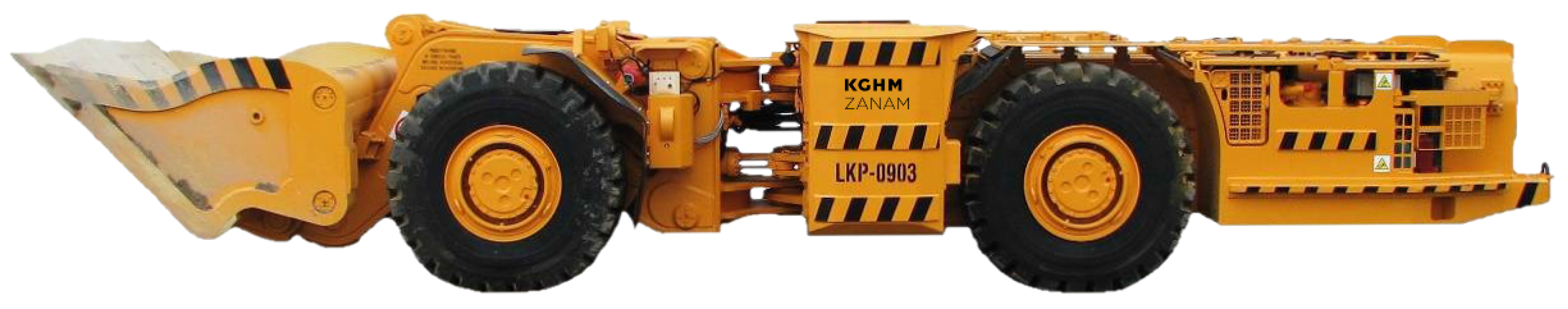
2.1. Machine Description
2.2. On Board Diagnostic System Description
2.3. Experiment Description
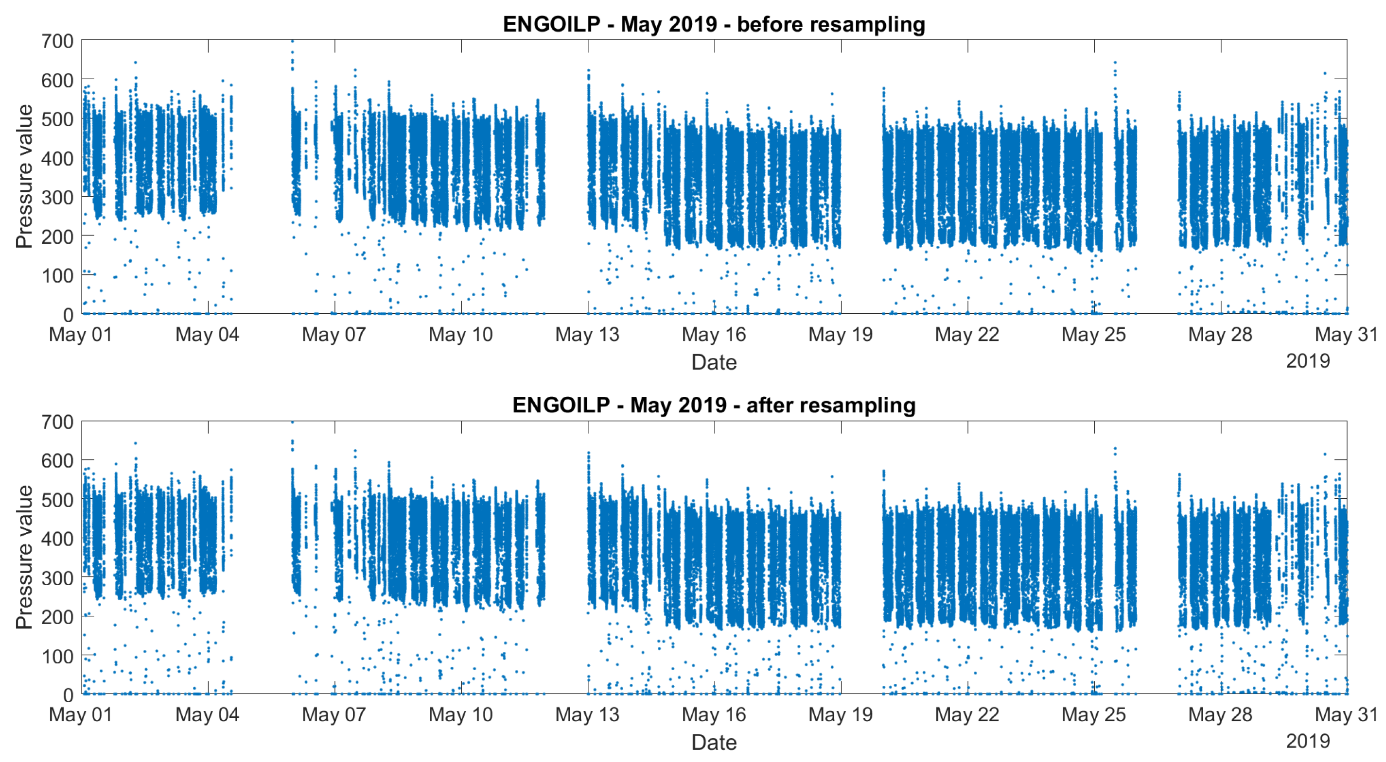
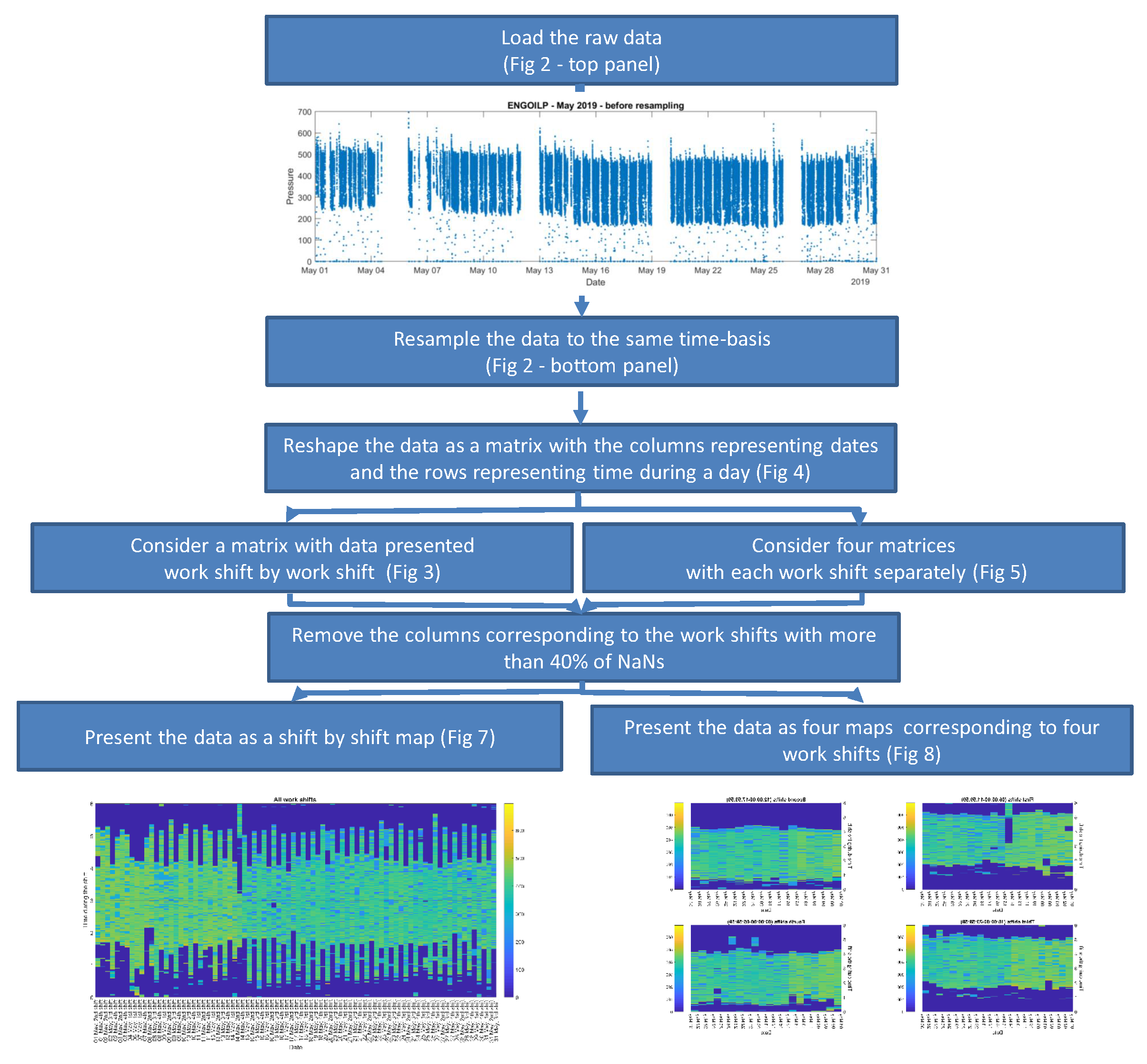
2.4. Data Pre-Processing
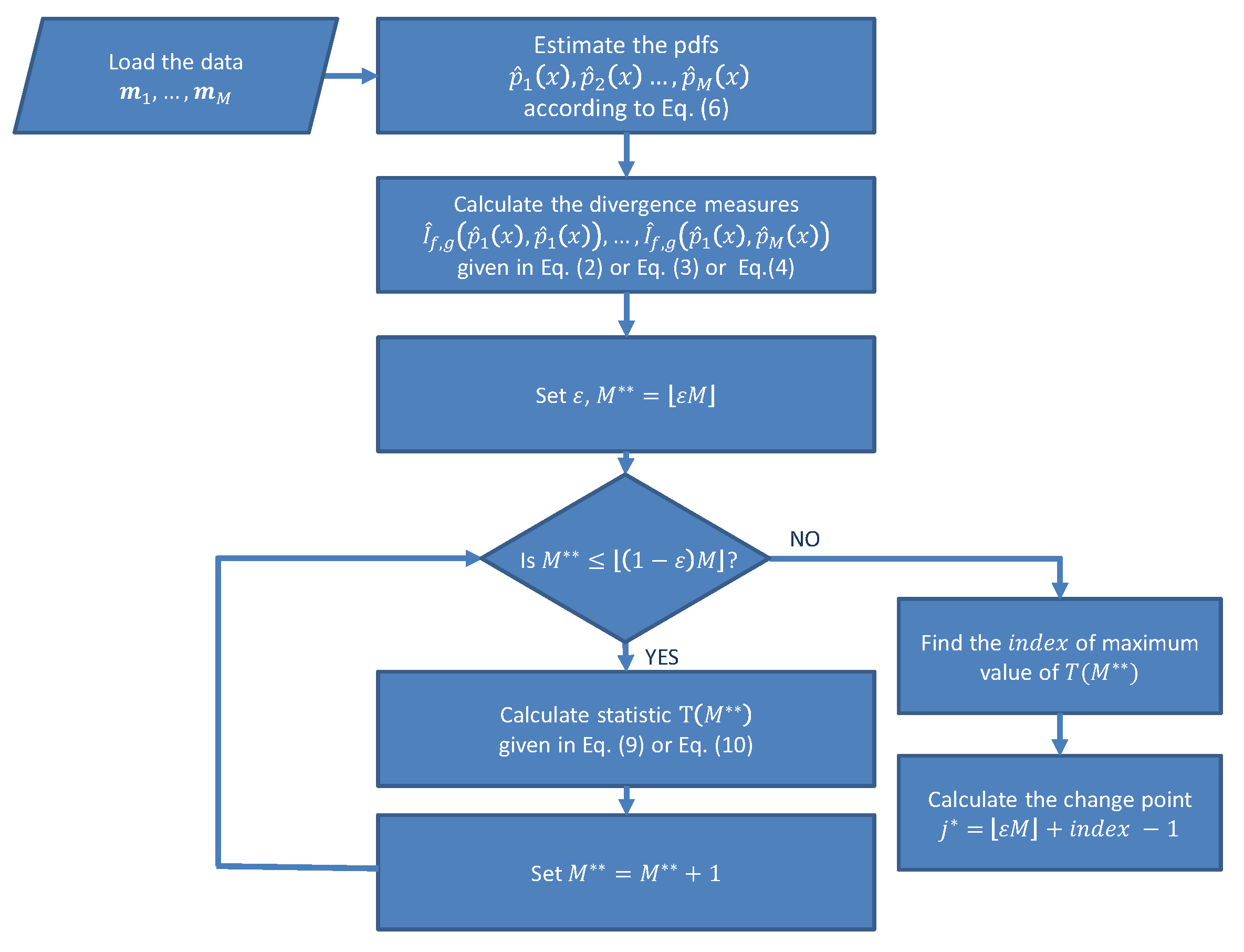
3. Methodology
4. Real Data Analysis
5. Discussion
6. Conclusions
- We have proposed a novel multistep procedure that covers pre-processing, statistical analysis, and visualization.
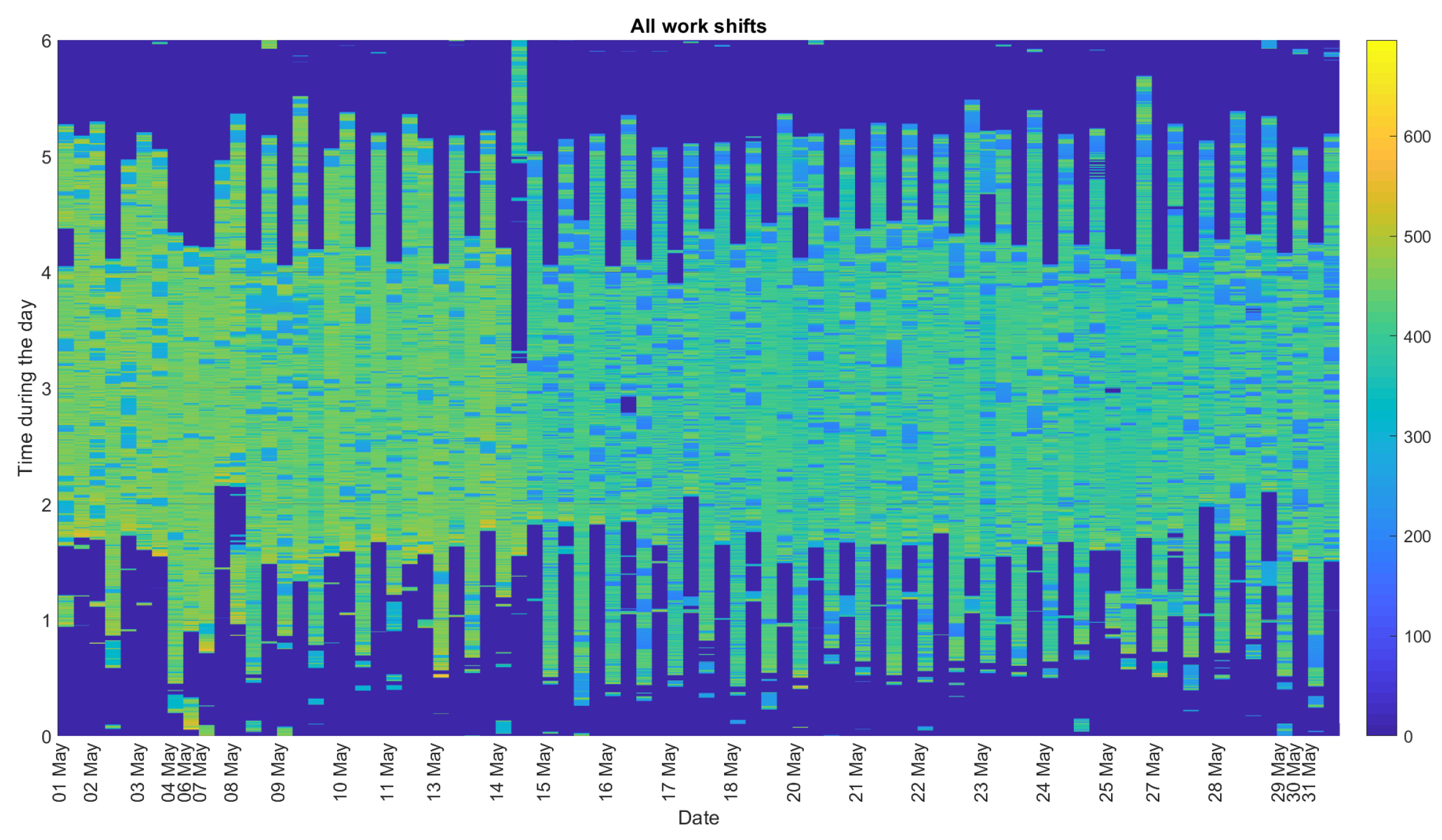
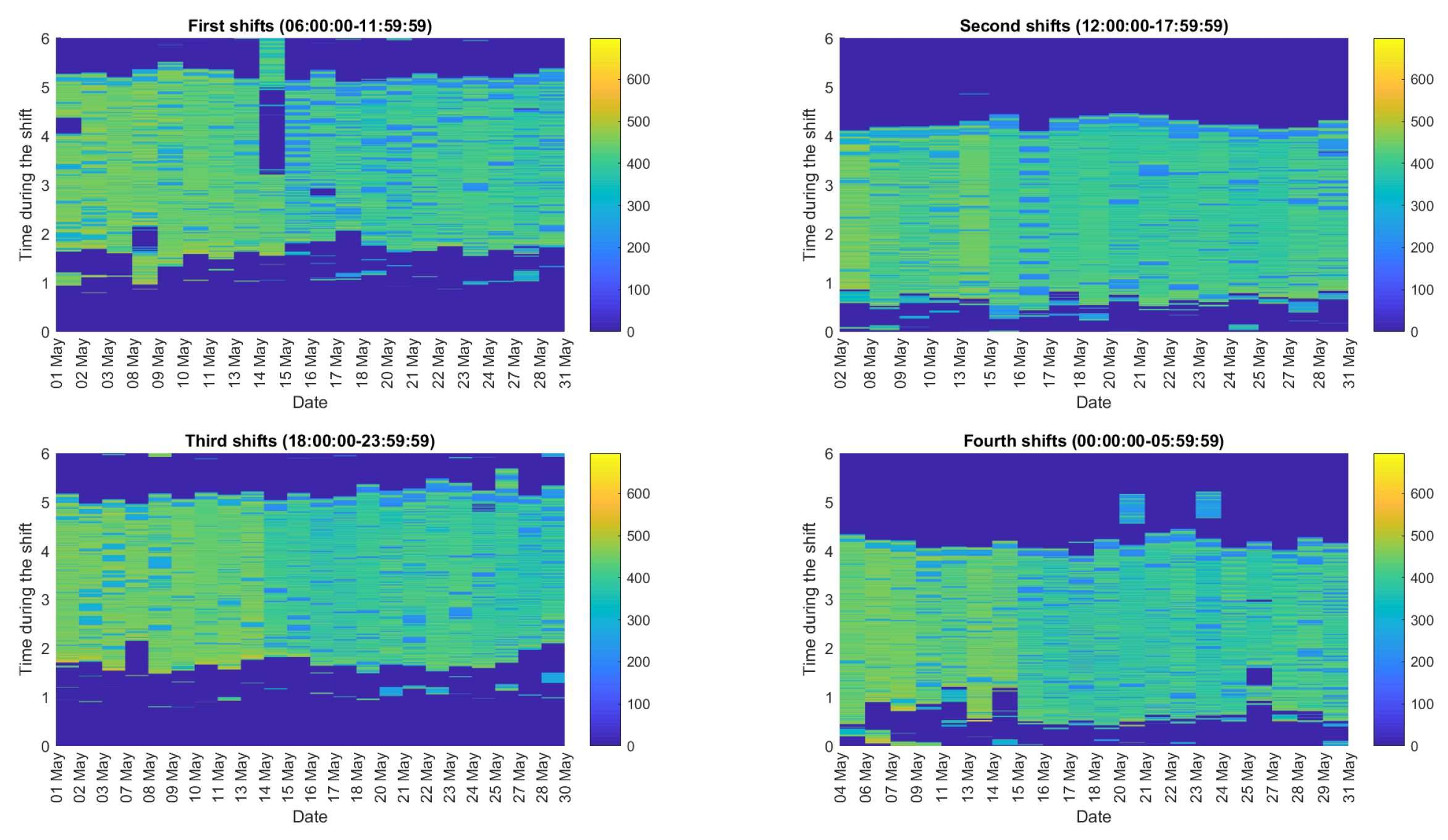
- The proposed procedure is the novel one. The innovation is related to the combination of the crucial steps of the proposed methodology, namely, the initial segmentation and the representation as a matrix in the work shift perspective as well as the analysis of the characteristics of the data (probability density functions) and the distance measures based on them. Finally, the last step (segmentation) is performed not for the real data, but for the distance measures of the time series’ pdfs. According to our knowledge, this approach is rarely used in real applications.
- The utilization of the distance measures of time series’ pdfs causes that we do not consider here the problem when one parameter of the data changes (like mean or variance). The examined issue is much more general. The analysis of the pdf’s changes causes the algorithm is sensitive to the dynamics of various characteristics of the data, not only the single one.
- The proposed approach is a universal one. It can be used for any cycle that corresponds to the considered phenomena (in our case it is a work shift), to any characteristics of the data (in our case it is the probability density function), and to any distance measure applied to the characteristics (in our case there are distance measures based on the probability density functions).
- The whole procedure is automatic, thus we believe it could be implemented in the monitoring systems used in the company. When the new data corresponding to the next day (four work shifts) come, then using the introduced procedure we can test if they belong to the current regime. In our case, the new sample means the data corresponding to the next day. This approach is often used in monitoring systems. Thus, in some sense, the methodology can be used in a continuous manner.
- The historical data with precise knowledge about replacement has been used for training and validation. Implementation of the proposed method as an automatic data processing procedure should not be a problem for any new machine. Small dataset from a couple of shifts from a new machine (new data set) will be enough to establish the averaged picture of the signature of good condition. If the damage will appear (change of regime), the method will be able to detect it after a few work shifts (min. 2), that is much better than the current situation. Note that a machine with such damage was able to operate for two weeks as there was not a tool to detect the problem.
- It should be highlighted, the proposed methodology has also some limitations. One of this is related to the special requirements of the data. More precisely, there is a need to consider data that could be arranged as work shifts (or any other cycles). This influences the identified structure break point corresponds to the work shift, not the real time point (like hour).
Author Contributions
Funding
Institutional Review Board Statement
Informed Consent Statement
Data Availability Statement
Conflicts of Interest
Appendix A. Tables

| Variable Name | Description |
|---|---|
| Temperatures | |
| ’ENGCOOLT’ | temperature of the cooling liquid of the internal combustion engine |
| ’GROILT’ | oil temperature of transmission and torque |
| ’HYDOILT’ | hydraulic oil temperature |
| Pressures | |
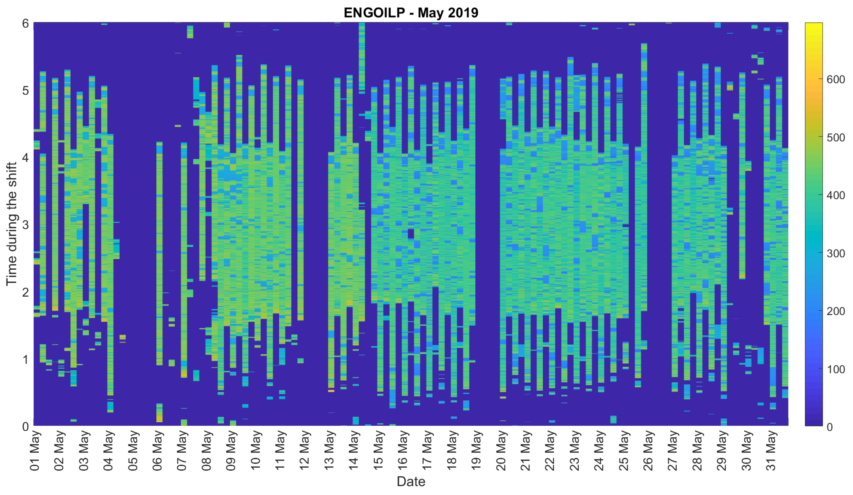
| ’ENGOILP’ | oil pressure of the internal combustion engine |
| ’BREAKP’ | breaking pressure |
| ’GROILP’ | transmission oil pressure |
| ’HYDOILP’ | pressure in the hydraulic system |
| Others | |
| ’ENGRPM’ | engine speed |
| ’FUELUS’ | instant fuel consumption |
| ’SELGEAR’ | direction and current gear |
| ’SPEED’ | average speed every 1s |
| Hellinger Distance | |
|---|---|
| Student’s t | Wilcoxon |
| 1st shift on | 1st shift on |
| 14th of May | 14th of May |
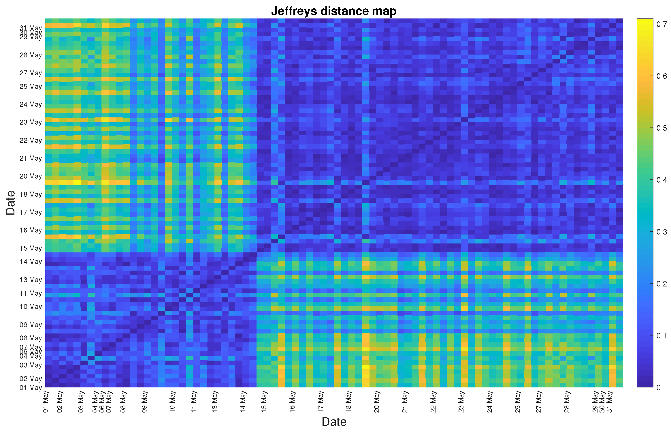
| Jeffreys distance | |
| Student’s t | Wilcoxon |
| 1st shift on | 1st shift on |
| 14th of May | 14th of May |
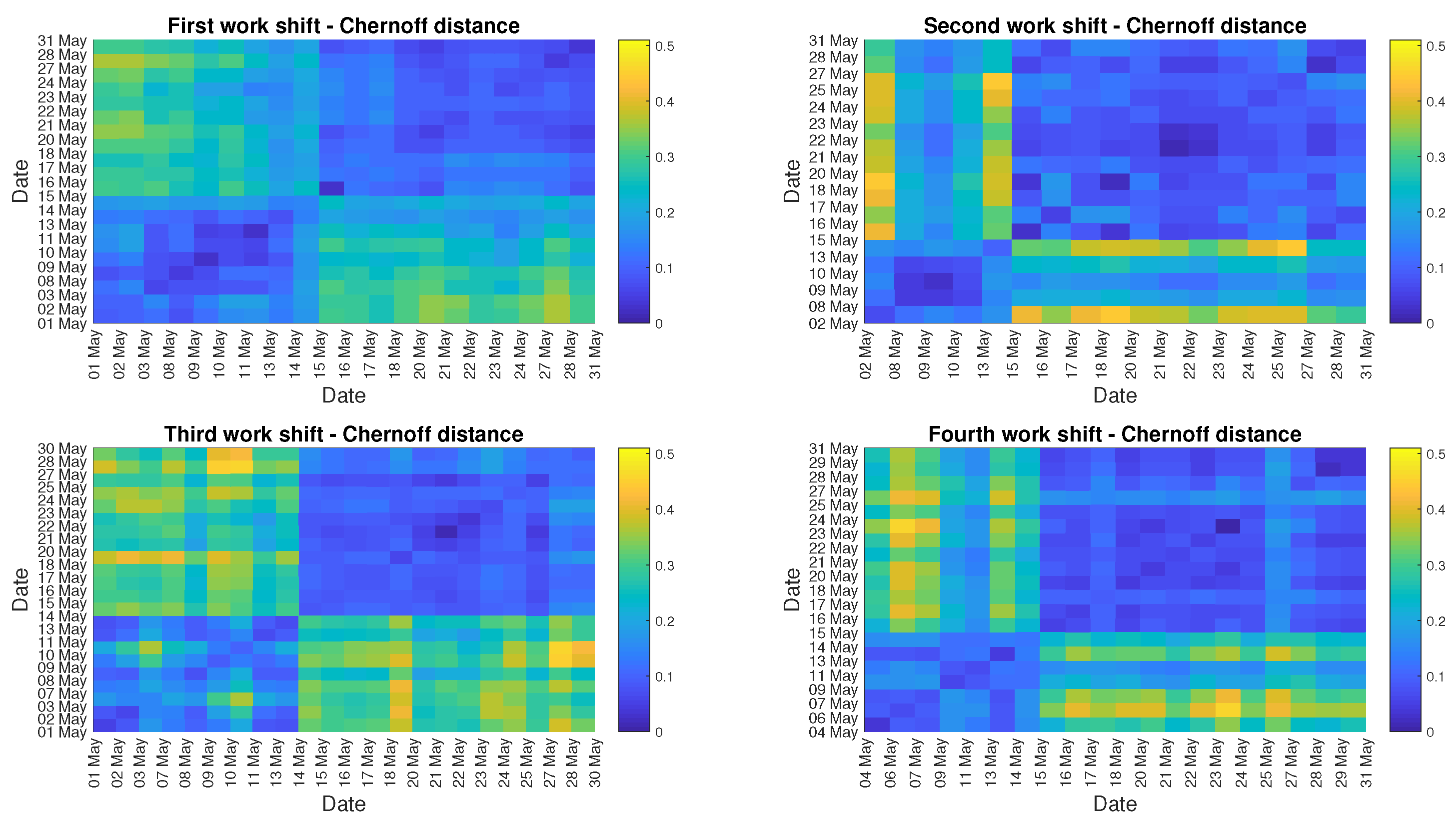
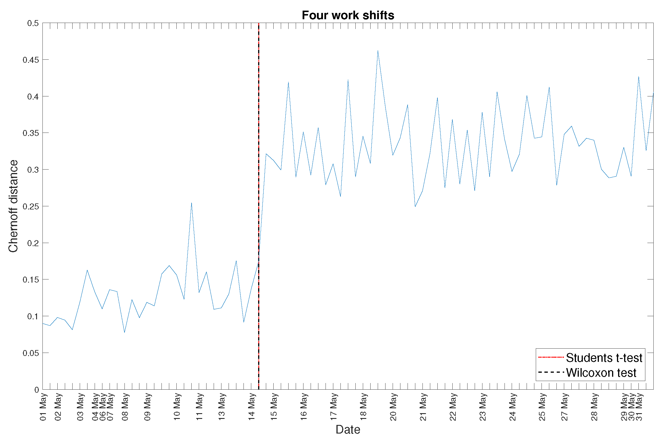
| Chernoff distance | |
| Student’s t | Wilcoxon |
| 1st shift on | 1st shift on |
| 14th of May | 14th of May |
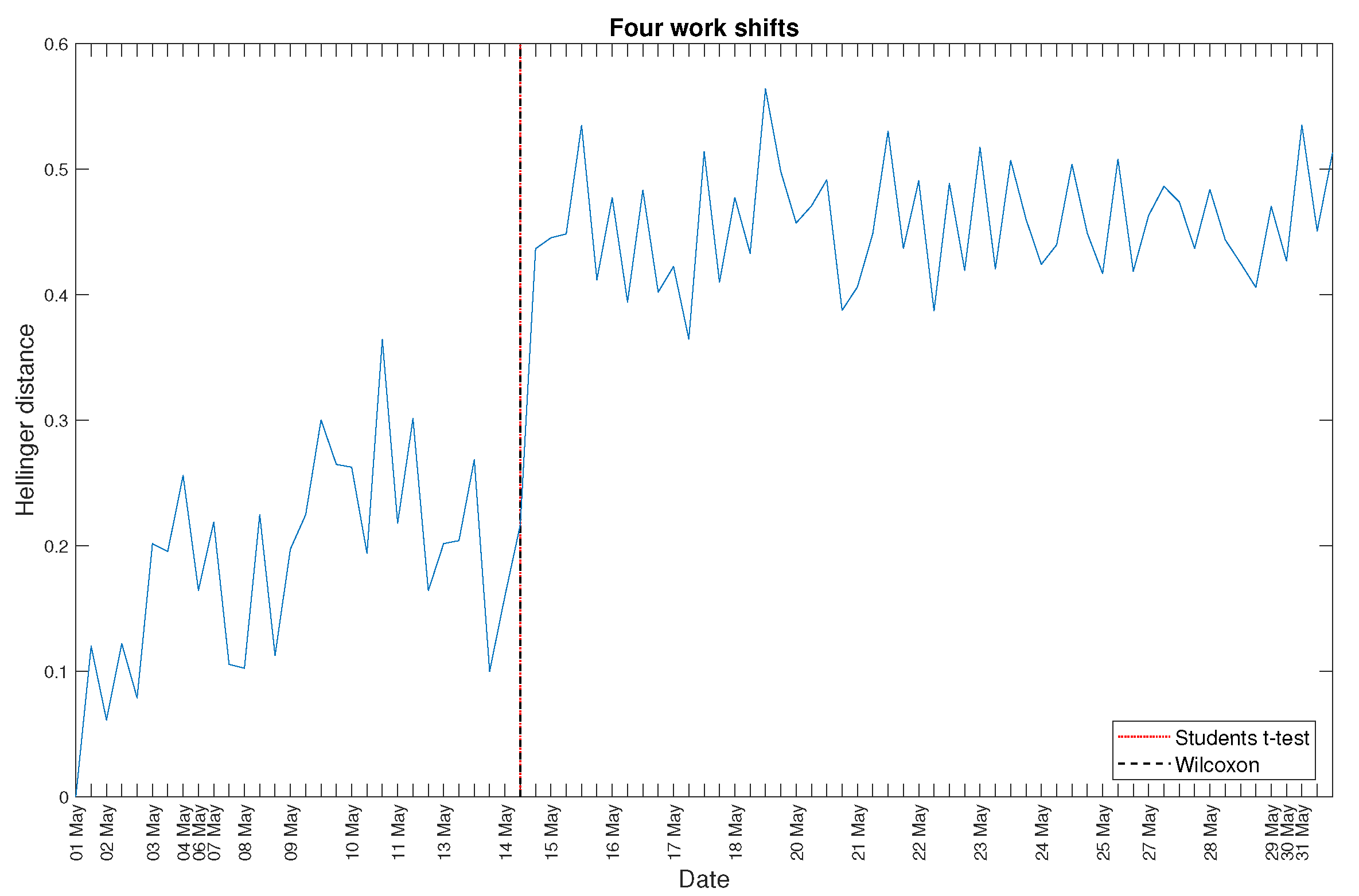
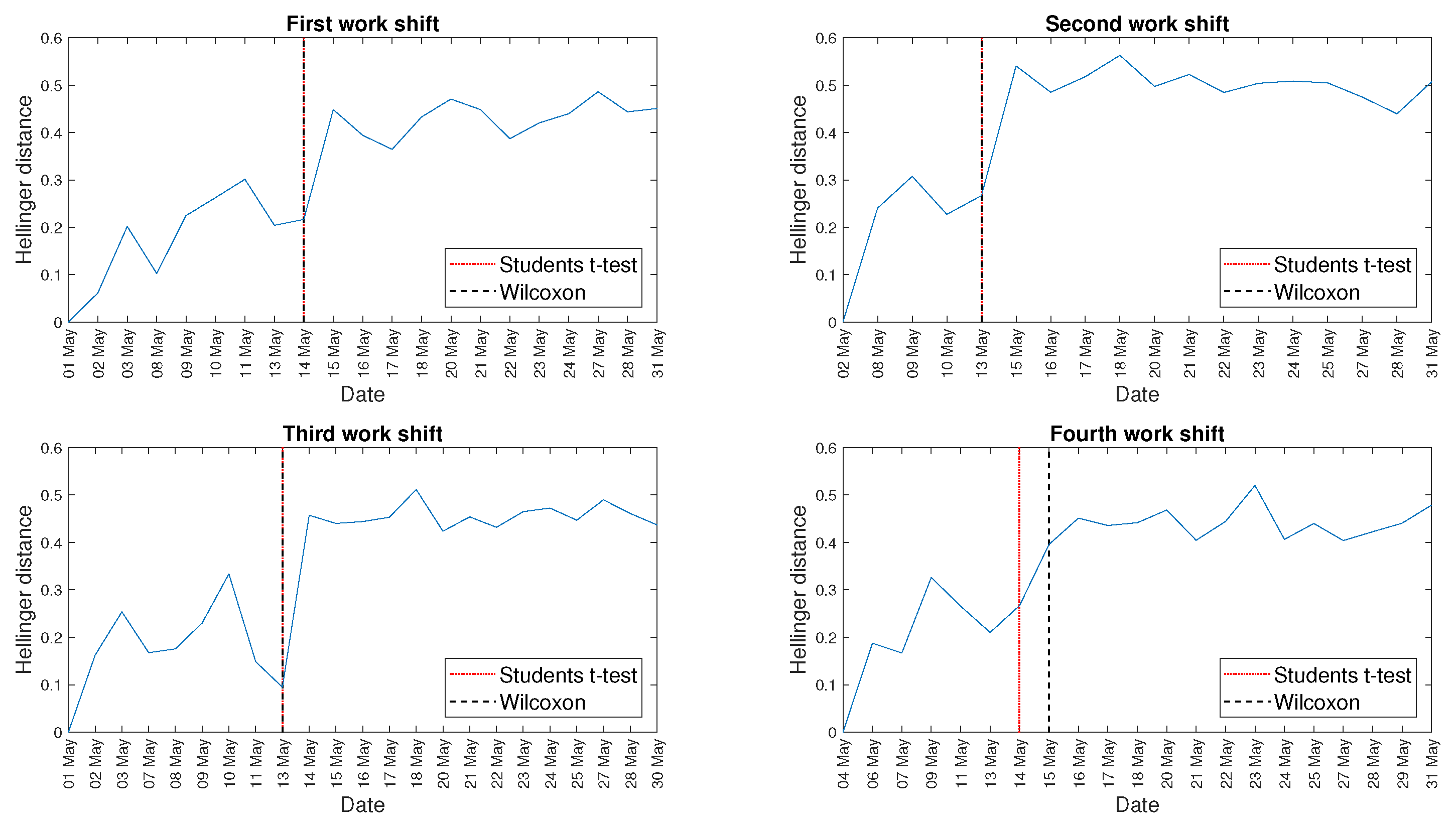
| Hellinger Distance | |
|---|---|
| First Shift | |
| Student’s t | Wilcoxon |
| 14th of May | 14th of May |
| Second shift | |
| Student’s t | Wilcoxon |
| 13th of May | 13th of May |
| Third shift | |
| Student’s t | Wilcoxon |
| 13th of May | 13th of May |
| Fourth shift | |
| Student’s t | Wilcoxon |
| 14th of May | 15th of May |
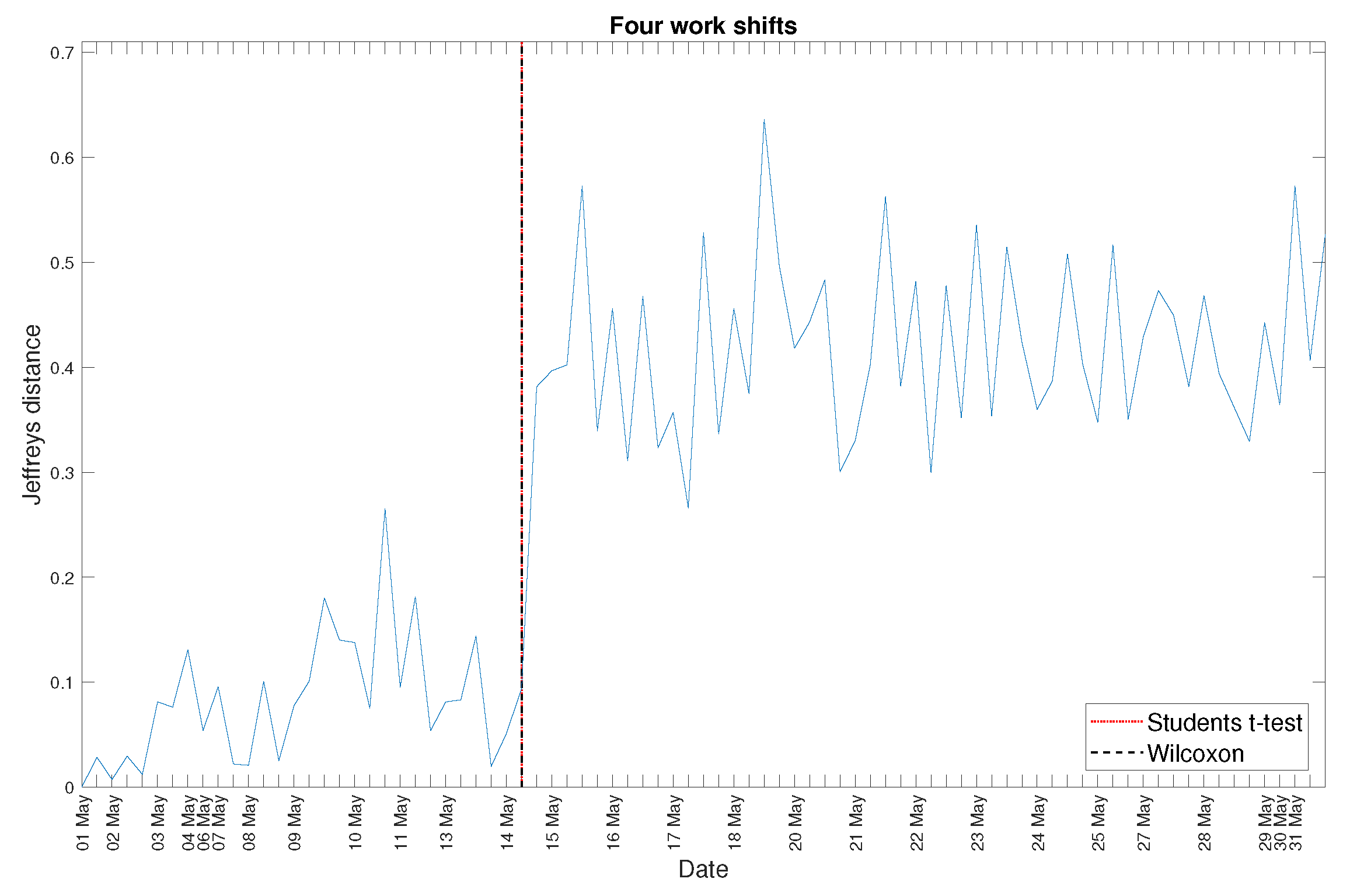
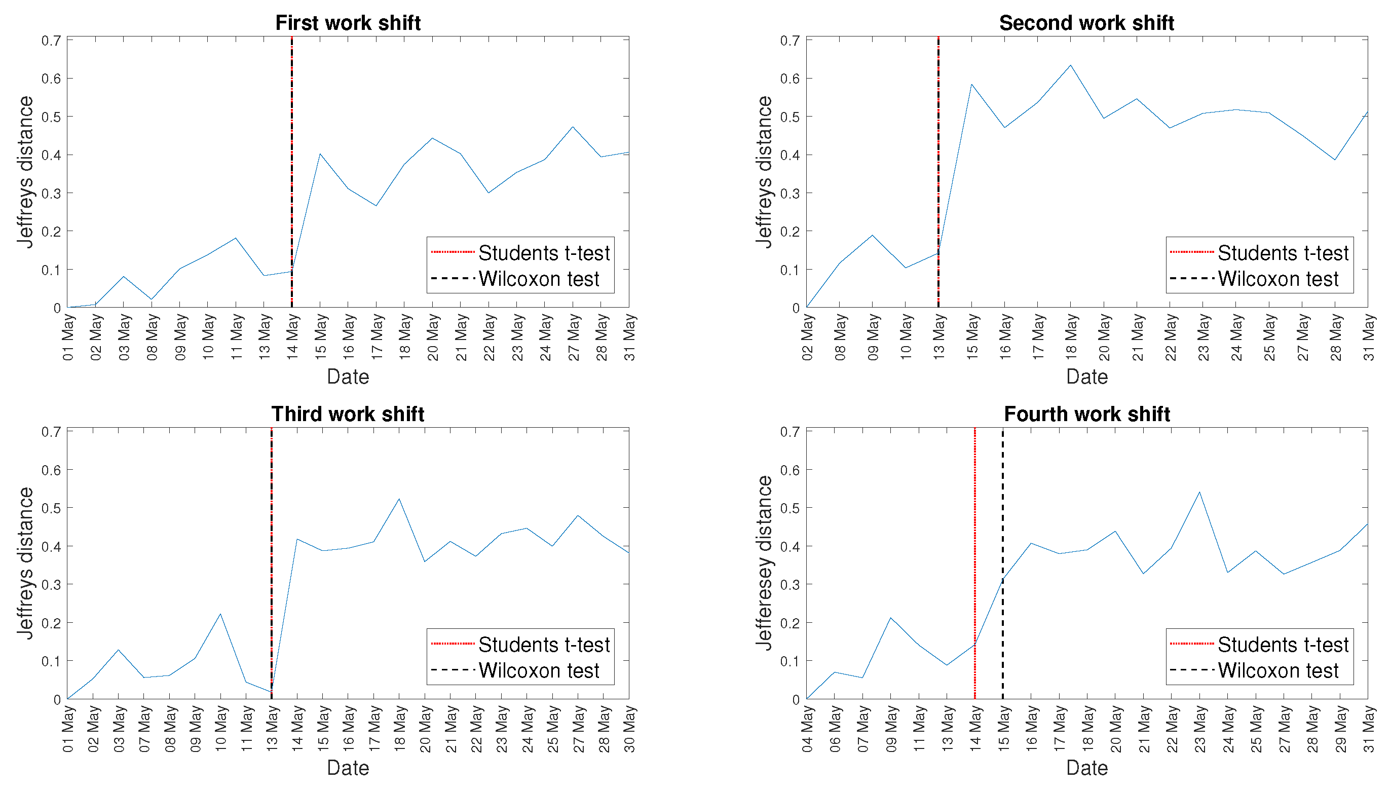
| Jeffreys Distance | |
|---|---|
| First Shift | |
| Student’s t | Wilcoxon |
| 14th of May | 14th of May |
| Second shift | |
| Student’s t | Wilcoxon |
| 13th of May | 13th of May |
| Third shift | |
| Student’s t | Wilcoxon |
| 13th of May | 13th of May |
| Fourth shift | |
| Student’s t | Wilcoxon |
| 14th of May | 15th of May |
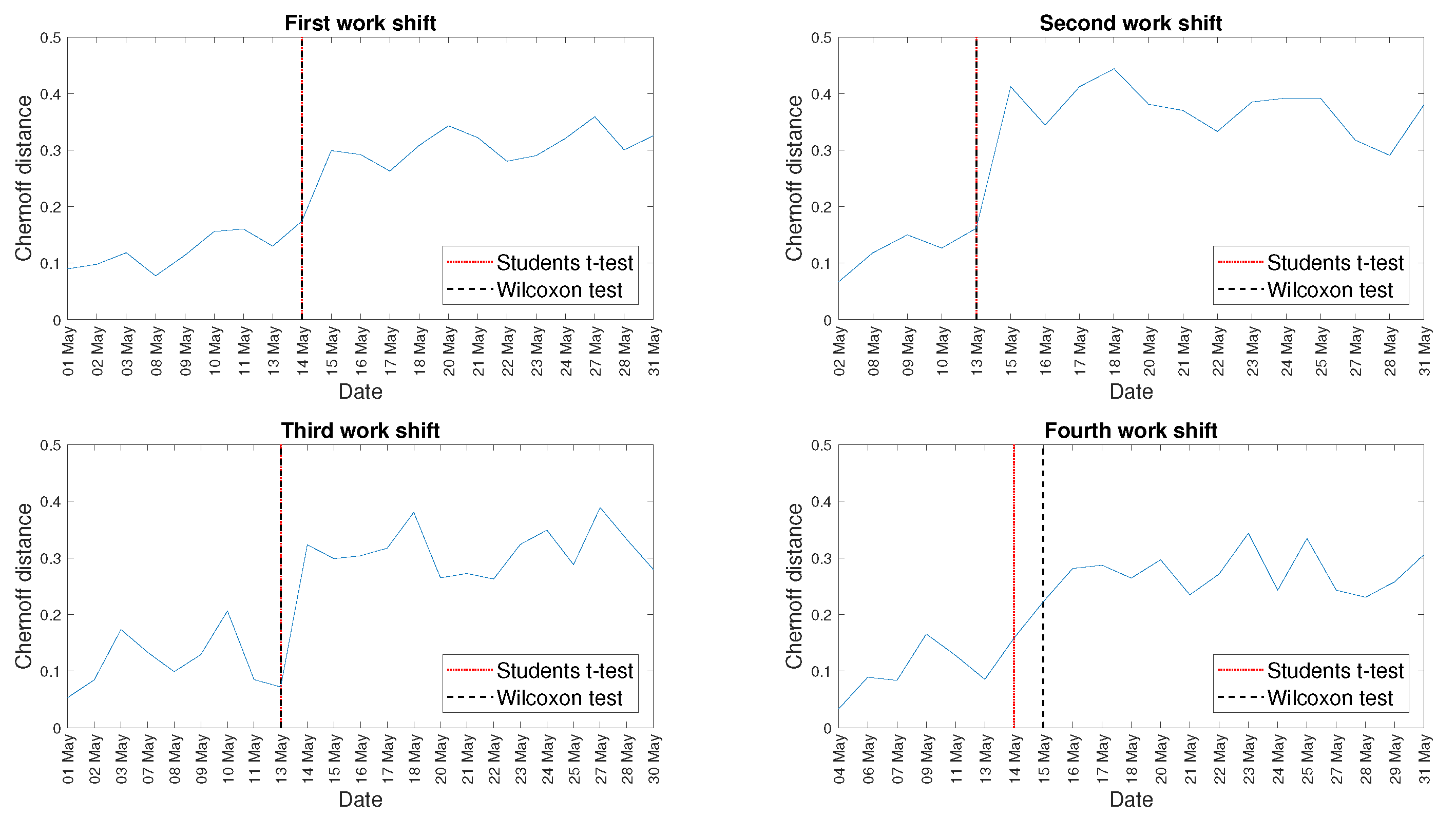
| Chernoff Distance | |
|---|---|
| First Shift | |
| Student’s t | Wilcoxon |
| 14th of May | 14th of May |
| Second shift | |
| Student’s t | Wilcoxon |
| 13th of May | 13th of May |
| Third shift | |
| Student’s t | Wilcoxon |
| 13th of May | 13th of May |
| Fourth shift | |
| Student’s t | Wilcoxon |
| 14th of May | 15th of May |
Appendix B. Additional Graphs


References
- Vashistha, S.; Kumar Agrawal, A.; Siddiqui, M.; Chattopadhyaya, S. Reliability and Maintainability Analysis of LHD Loader at Saoner Mines, Nagpur, India. IOP Conf. Ser. Mater. Sci. Eng. 2019, 691, 012013. [Google Scholar] [CrossRef]
- Jakkula, B.; Govinda Raj, M.; Murthy, C. Maintenance management of load haul dumper using reliability analysis. J. Qual. Maint. Eng. 2019, 26, 290–310. [Google Scholar] [CrossRef]
- Chatterjee, S.; Bandopadhyay, S. Reliability estimation using a genetic algorithm-based artificial neural network: An application to a load-haul-dump machine. Expert Syst. Appl. 2012, 39, 10943–10951. [Google Scholar] [CrossRef]
- Dindarloo, S. Reliability forecasting of a load-haul-dump machine: A comparative study of ARIMA and neural networks. Qual. Reliab. Eng. Int. 2016, 32, 1545–1552. [Google Scholar] [CrossRef]
- Bala, R.; Govinda, R.; Murthy, C. Reliability analysis and failure rate evaluation of load haul dump machines using Weibull distribution analysis. Math. Model. Eng. Probl. 2018, 5, 116–122. [Google Scholar] [CrossRef]
- Paithankar, A.; Chatterjee, S. Forecasting time-to-failure of machine using hybrid Neuro-genetic algorithm–a case study in mining machinery. Int. J. Mining Reclam. Environ. 2018, 32, 182–195. [Google Scholar] [CrossRef]
- Balaraju, J.; Govinda Raj, M.; Murthy, C.S.N. Prediction and Assessment of LHD Machine Breakdowns Using Failure Mode Effect Analysis (FMEA). In Reliability, Safety and Hazard Assessment for Risk-Based Technologies; Varde, P.V., Prakash, R.V., Vinod, G., Eds.; Springer: Singapore, 2020; pp. 833–850. [Google Scholar]
- Jakkula, B.; Mandela, G.; Chivukula, S. Application ANN Tool for Validation of LHD Machine Performance Characteristics. J. Inst. Eng. (India) Ser. D 2020, 101, 27–38. [Google Scholar] [CrossRef]
- Jakkula, B.; Mandela, G.; Chivukula, M. Improvement of overall equipment performance of underground mining machines- a case study. Adv. Model. Anal. A 2018, 79, 6–11. [Google Scholar] [CrossRef]
- Jakobs, A. The Sandvik LH621, from hardrock loader to high-performance machine in German salt and potash mining. World Min. Surf. Undergr. 2018, 70, 276–279. [Google Scholar]
- Mkhwanazi, D. Optimizing LHD utilization. J. South Afr. Inst. Min. Metall. 2011, 111, 273–280. [Google Scholar]
- Krot, P.; Śliwiński, P.; Zimroz, R.; Gomolla, N. The identification of operational cycles in the monitoring systems of underground vehicles. Measurement 2020, 151, 107111. [Google Scholar] [CrossRef]
- Mbhalati, W. LHD optimization at an underground chromite mine. J. South Afr. Inst. Min. Metall. 2015, 115, 313–320. [Google Scholar] [CrossRef]
- Fukui, R.; Kusaka, K.; Nakao, M.; Kodama, Y.; Uetake, M.; Kawai, K. Production analysis of functionally distributed machines for underground mining. Int. J. Min. Sci. Technol. 2016, 26, 477–485. [Google Scholar] [CrossRef]
- Stefaniak, P.; Zimroz, R.; Obuchowski, J.; Śliwiński, P.; Andrzejewski, M. An Effectiveness Indicator for a Mining Loader Based on the Pressure Signal Measured at a Bucket’s Hydraulic Cylinder. Procedia Earth Planet. Sci. 2015, 15, 797–805. [Google Scholar] [CrossRef]
- Balaraju, J.; Govinda Raj, M.; Murthy, C. Fuzzy-FMEA risk evaluation approach for LHD machine—A case study. J. Sustain. Min. 2019, 18, 257–268. [Google Scholar] [CrossRef]
- Ghodrati, B.; Hoseinie, S.; Kumar, U. Context-driven mean residual life estimation of mining machinery. Int. J. Mining Reclam. Environ. 2018, 32, 486–494. [Google Scholar] [CrossRef]
- Laukka, A.; Saari, J.; Ruuska, J.; Juuso, E.; Lahdelma, S. Condition-based monitoring for underground mobile machines. Int. J. Ind. Syst. Eng. 2016, 23, 74–89. [Google Scholar] [CrossRef]
- Zimroz, R.; Wodecki, J.; Król, R.; Andrzejewski, M.; Śliwiński, P.; Stefaniak, P. Self-propelled Mining Machine Monitoring System—Data Validation, Processing and Analysis. In Mine Planning and Equipment Selection; Drebenstedt, C., Singhal, R., Eds.; Springer International Publishing: Cham, Switzerland, 2014; pp. 1285–1294. [Google Scholar]
- Wodecki, J.; Stefaniak, P.; Michalak, A.; Wyłomańska, A.; Zimroz, R. Technical condition change detection using Anderson-Darling statistic approach for LHD machines—Engine overheating problem. Int. J. Mining Reclam. Environ. 2018, 32, 392–400. [Google Scholar] [CrossRef]
- Michalak, A.; Śliwiński, P.; Kaniewski, T.; Wodecki, J.; Stefaniak, P.; Wyłomańska, A.; Zimroz, R. Condition Monitoring for LHD Machines Operating in Underground Mine—Analysis of Long-Term Diagnostic Data. In Proceedings of the 27th International Symposium on Mine Planning and Equipment Selection—MPES 2018; Widzyk-Capehart, E., Hekmat, A., Singhal, R., Eds.; Springer International Publishing: Cham, Switzerland, 2019; pp. 471–480. [Google Scholar]
- Stefaniak, P.; Śliwiński, P.; Poczynek, P.; Wyłomańska, A.; Zimroz, R. The Automatic Method of Technical Condition Change Detection for LHD Machines—Engine Coolant Temperature Analysis. In Advances in Condition Monitoring of Machinery in Non-Stationary Operations; Fernandez Del Rincon, A., Viadero Rueda, F., Chaari, F., Zimroz, R., Haddar, M., Eds.; Springer International Publishing: Cham, Switzerland, 2019; pp. 54–63. [Google Scholar]
- Paraszczak, J.; Gustafson, A.; Schunnesson, H. Technical and operational aspects of autonomous LHD application in metal mines. Int. J. Mining Reclam. Environ. 2015, 29, 391–403. [Google Scholar]
- Gustafson, A.; Paraszczak, J.; Tuleau, J.; Schunnesson, H. Impact of technical and operational factors on effectiveness of automatic load-haul-dump machines. Trans. Institutions Min. Metall. Sect. A Min. Technol. 2017, 126, 185–190. [Google Scholar]
- Kaniewski, T.; Śliwiński, P.; Hebda-Sobkowicz, J.; Zimroz, R. Comprehensive, experimental verification of the effects of the lock-up function implementation in LHD haul trucks in the deep underground mine. In Proceedings of the Mining Goes Digital: Proceedings of the 39th International Symposium on Application of Computers and Operations Research in the Mineral Industry (APCOM 2019), Wrocław, Poland, 4–6 June 2019; pp. 506–514. [Google Scholar]
- Śliwiński, P.; Kaniewski, T.; Hebda-Sobkowicz, J.; Zimroz, R.; Wyłomańska, A. Analysis of dynamic external loads to haul truck machine subsystems during operation in a deep underground mine. In Proceedings of the Mining Goes Digital: Proceedings of the 39th International Symposium on Application of Computers and Operations Research in the Mineral Industry (APCOM 2019), Wrocław, Poland, 4–6 June 2019; pp. 515–524. [Google Scholar]
- Wang, Y.; Jin, T.; Liu, L. Output torque prediction of hybrid underground LHD motor based on least square support vector machine. Meitan Xuebao J. China Coal Soc. 2017, 42, 619–625. [Google Scholar]
- Saari, J.; Odelius, J. Detecting operation regimes using unsupervised clustering with infected group labelling to improve machine diagnostics and prognostics. Oper. Res. Perspect. 2018, 5, 232–244. [Google Scholar] [CrossRef]
- Wyłomańska, A.; Zimroz, R. Signal segmentation for operational regimes detection of heavy duty mining mobile machines-a statistical approach. Diagnostyka 2014, 15, 33–42. [Google Scholar]
- Wodecki, J.; Michalak, A.; Stefaniak, P. Review of smoothing methods for enhancement of noisy data from heavy-duty LHD mining machines. E3S Web Conf. 2018, 29, 00011. [Google Scholar] [CrossRef]
- Stefaniak, P.K.; Zimroz, R.; Śliwiński, P.; Andrzejewski, M.; Wyłomańska, A. Multidimensional Signal Analysis for Technical Condition, Operation and Performance Understanding of Heavy Duty Mining Machines. In Advances in Condition Monitoring of Machinery in Non-Stationary Operations; Chaari, F., Zimroz, R., Bartelmus, W., Haddar, M., Eds.; Springer International Publishing: Cham, Switzerland, 2016; pp. 197–210. [Google Scholar]
- Śliwiński, P.; Andrzejewski, M.; Kaniewski, T.; Hebda-Sobkowicz, J.; Zimroz, R. Selection of variables acquired by the on-board monitoring system to determine operational cycles for haul truck vehicle. In Proceedings of the Mining Goes Digital: Proceedings of the 39th International Symposium on Application of Computers and Operations Research in the Mineral Industry (APCOM 2019), Wrocław, Poland, 4–6 June 2019; pp. 525–533. [Google Scholar]
- Kucharczyk, D.; Wyłomańska, A.; Zimroz, R. Structural break detection method based on the Adaptive Regression Splines technique. Physica A 2017, 471, 499–511. [Google Scholar] [CrossRef]
- Obuchowski, J.; Wyłomańska, A.; Zimroz, R. The local maxima method for enhancement of time-frequency map and its application to local damage detection in rotating machines. Mech. Syst. Signal Process. 2014, 46, 389–405. [Google Scholar] [CrossRef]
- Andreao, R.V.; Dorizzi, B.; Boudy, J. ECG signal analysis through hidden Markov models. IEEE Trans. Biomed. Eng. 2006, 53, 1541–1549. [Google Scholar] [CrossRef] [PubMed]
- Azami, H.; Mohammadi, K.; Bozorgtabar, B. An Improved Signal Segmentation Using Moving Average and Savitzky-Golay Filter. J. Signal Inf. Process. 2012, 3, 39–44. [Google Scholar]
- Bhagavatula, C.; Jaech, A.; Savvides, M.; Bhagavatula, V.; Friedman, R.; Blue, R.; O Griofa, M. Automatic segmentation of cardiosynchronous waveforms using cepstral analysis and continuous wavelet transforms. In Proceedings of the 19th IEEE International Conference on Image Processing, Orlando, FL, USA, 30 September–3 October 2012; pp. 2045–2048. [Google Scholar]
- Choi, S.; Jiang, Z. Comparison of envelope extraction algorithms for cardiac sound signal segmentation. Expert Syst. Appl. 2008, 34, 1056–1069. [Google Scholar] [CrossRef]
- Micó, P.; Mora, M.; Cuesta-Frau, D.; Aboy, M. Automatic segmentation of long-term ECG signals corrupted with broadband noise based on sample entropy. Comput. Methods Programs Biomed. 2010, 98, 118–129. [Google Scholar] [CrossRef]
- Khanagha, V.; Daoudi, K.; Pont, O.; Yahia, H. Phonetic segmentation of speech signal using local singularity analysis. Digit. Signal Process. 2014, 35, 86–94. [Google Scholar] [CrossRef]
- Lovell, B.; Boashash, B. Segmentation of non-stationary signals with applications. In Proceedings of the International Conference on Acoustics, Speech, and Signal Processing, New York, NY, USA, 11–14 April 1988; Volume 5, pp. 2685–2688. [Google Scholar]
- Makowski, R.; Hossa, R. Automatic speech signal segmentation based on the innovation adaptive filter. Int. J. Appl. Math. Comput. Sci. 2014, 24, 259–270. [Google Scholar] [CrossRef]
- Janczura, J.; Weron, R. Goodness-of-fit testing for the marginal distribution of regime-switching models with an application to electricity spot prices. AStA Adv. Stat. Anal. 2013, 97, 239–270. [Google Scholar] [CrossRef]
- Janczura, J. Pricing electricity derivatives within a Markov regime-switching model: A risk premium approach. Math. Methods Oper. Res. 2014, 79, 1–30. [Google Scholar] [CrossRef]
- Chen, C. On a segmentation algorithm for seismic signal analysis. Geoexploration 1984, 23, 35–40. [Google Scholar] [CrossRef]
- Gaby, J.E.; Anderson, K.R. Hierarchical segmentation of seismic waveforms using affinity. Geoexploration 1984, 23, 1–16. [Google Scholar] [CrossRef]
- Kucharczyk, D.; Wyłomańska, A.; Obuchowski, J.; Zimroz, R.; Madziarz, M. Stochastic Modelling as a Tool for Seismic Signals Segmentation. Shock Vib. 2016, 2016, 1–13. [Google Scholar] [CrossRef]
- Popescu, T.D. Signal segmentation using changing regression models with application in seismic engineering. Digit. Signal Process. 2014, 24, 14–26. [Google Scholar] [CrossRef]
- Sokołowski, J.; Obuchowski, J.; Zimroz, R.; Wyłomańska, A.; Koziarz, E. Algorithm Indicating Moment of P-Wave Arrival Based on Second-Moment Characteristic. Shock Vib. 2016, 2016, 1–6. [Google Scholar] [CrossRef]
- Gajda, J.; Sikora, G.; Wyłomańska, A. Regime Variance Testing—A Quantile Approach. Acta Phys. Pol. B Proc. Suppl. 2013, 44, 1015–1035. [Google Scholar] [CrossRef]
- Makowski, R.; Zimroz, R. New techniques of local damage detection in machinery based on stochastic modelling using adaptive Schur filter. Appl. Acoust. 2014, 77, 130–137. [Google Scholar] [CrossRef]
- Makowski, R.; Zimroz, R. A procedure for weighted summation of the derivatives of reflection coefficients in adaptive Schur filter with application to fault detection in rolling element bearings. Mech. Syst. Signal Process. 2013, 38, 65–77. [Google Scholar] [CrossRef]
- Tsay, R.S. Outliers, level shifts, and variance changes in time series. J. Forecast. 1988, 7, 1–20. [Google Scholar] [CrossRef]
- Urbanek, J.; Barszcz, T.; Zimroz, R.; Antoni, J. Application of averaged instantaneous power spectrum for diagnostics of machinery operating under non-stationary operational conditions. Measurement 2012, 45, 1782–1791. [Google Scholar] [CrossRef]
- Lanoiselée, Y.; Grebenkov, D. Unraveling intermittent features in single-particle trajectories by a local convex hull method. Phys. Rev. E 2017, 96, 022144. [Google Scholar] [CrossRef]
- Wagner, T.; Kroll, A.; Haramagatti, C.R.; Lipinski, H.G.; Wiemann, M. Classification and Segmentation of Nanoparticle Diffusion Trajectories in Cellular Micro Environments. PLoS ONE 2017, 12, 1–20. [Google Scholar]
- Akimoto, T.; Yamamoto, E. Detection of transition times from single-particle-tracking trajectories. Phys. Rev. E 2017, 96, 052138. [Google Scholar] [CrossRef]
- Sikora, G.; Wyłomańska, A.; Krapf, D. Recurrence statistics for anomalous diffusion regime change detection. Comput. Stat. Data Anal. 2018, 128, 380–394. [Google Scholar] [CrossRef]
- Sikora, G.; Wyłomańska, A.; Gajda, J.; Solé, L.; Akin, E.; Tamkun, M.; Krapf, D. Elucidating distinct ion channel populations on the surface of hippocampal neurons via single-particle tracking recurrence analysis. Phys. Rev. E 2017, 96, 062404. [Google Scholar] [CrossRef]
- Li, W.; Li, H.; Gu, S.; Chen, T. Process fault diagnosis with model- and knowledge-based approaches: Advances and opportunities. Control. Eng. Pract. 2020, 105, 104637. [Google Scholar] [CrossRef]
- Qin, S. Survey on data-driven industrial process monitoring and diagnosis. Annu. Rev. Control. 2012, 36, 220–234. [Google Scholar] [CrossRef]
- Yan, Y.; Li, J.; Gao, D. Condition parameter modeling for anomaly detection in wind turbines. Energies 2014, 7, 3104–3120. [Google Scholar] [CrossRef]
- Aghabozorgi, S.; Seyed Shirkhorshidi, A.; Ying Wah, T. Time-series clustering—A decade review. Inf. Syst. 2015, 53, 16–38. [Google Scholar] [CrossRef]
- Branisavljević, N.; Kapelan, Z.; Prodanović, D. Improved real-time data anomaly detection using context classification. J. Hydroinform. 2011, 13, 307–323. [Google Scholar] [CrossRef]
- Chandola, V.; Banerjee, A.; Kumar, V. Anomaly detection: A survey. ACM Comput. Surv. 2009, 41, 1–58. [Google Scholar] [CrossRef]
- Markou, M.; Singh, S. Novelty detection: A review—Part 1: Statistical approaches. Signal Process. 2003, 83, 2481–2497. [Google Scholar] [CrossRef]
- Myers, D.; Suriadi, S.; Radke, K.; Foo, E. Anomaly detection for industrial control systems using process mining. Comput. Secur. 2018, 78, 103–125. [Google Scholar] [CrossRef]
- Zhao, H.; Liu, H.; Hu, W.; Yan, X. Anomaly detection and fault analysis of wind turbine components based on deep learning network. Renew. Energy 2018, 127, 825–834. [Google Scholar] [CrossRef]
- Available online: https://www.kghmzanam.com/en/kategoria/mining-machinery/loaders/ (accessed on 27 July 2021).
- Csiszár, I. Information-Type Measures of Difference of Probability Distributions and Indirect Observations. Stud. Sci. Math. Hung. 1967, 2, 299–318. [Google Scholar]
- Csiszár, I. I-Divergence Geometry of Probability Distributions and Minimization Problem. Ann. Probab. 1975, 3, 146–158. [Google Scholar] [CrossRef]
- Basseville, M. Distance measures for signal processing and pattern recognition. Signal Process. 1989, 18, 349–369. [Google Scholar] [CrossRef]
- Basseville, M. Divergence measures for statistical data processing - An annotated bibliography. Signal Process. 2013, 93, 621–633. [Google Scholar] [CrossRef]
- Chung, J.; Kannappan, P.; Ng, C.; Sahoo, P. Measures of distance between probability distributions. J. Math. Anal. Appl. 1989, 138, 280–292. [Google Scholar] [CrossRef]
- Hill, P.D. Kernel estimation of a distribution function. Commun. Stat. Theory Methods 1985, 14, 605–620. [Google Scholar]
- Bowman, A.W.; Azzalini, A. Applied Smoothing Techniques for Data Analysis; Oxford University Press Inc.: New York, NY, USA, 1997. [Google Scholar]
- Silverman, B. Density Estimation: For Statistics and Data Analysis; Chapman & Hall: London, UK, 1986. [Google Scholar]
- Blair, R.C.; Higgins, J.J. A Comparison of the Power of Wilcoxon’s Rank-Sum Statistic to that of Student’st Statistic Under Various Nonnormal Distributions. J. Educ. Stat. 1980, 5, 309–335. [Google Scholar] [CrossRef]
- Rice, J.A. Mathematical Statistics and Data Analysis, 3rd ed.; Duxbury Press: Belmont, CA, USA, 2006. [Google Scholar]
- Hogg, R.; Craig, A. Introduction to Mathematical Statistics, 4th ed.; Macmillan: New York, NY, USA, 1978. [Google Scholar]
- Venables, W.N.; Ripley, B.D. Modern Applied Statistics with S, 4th ed.; Springer: New York, NY, USA, 2010. [Google Scholar]
- Fay, M.P.; Proschan, M.A. Wilcoxon-Mann-Whitney or t-test? On assumptions for hypothesis tests and multiple interpretations of decision rules. Stat. Surv. 2010, 4, 1–39. [Google Scholar] [CrossRef] [PubMed]
- Conover, W.J. Practical Nonparametric Statistics, 2nd ed.; Wiley: New York, NY, USA, 1980; pp. 225–226. [Google Scholar]
- Grzesiek, A.; Zimroz, R.; Śliwiński, P.; Gomolla, N.; Wyłomańska, A. Long term belt conveyor gearbox temperature data analysis—Statistical tests for anomaly detection. Measurement 2020, 165, 108124. [Google Scholar] [CrossRef]
- Urbanek, J.; Barszcz, T.; Straczkiewicz, M.; Jablonski, A. Normalization of vibration signals generated under highly varying speed and load with application to signal separation. Mech. Syst. Signal Process. 2017, 82, 13–31. [Google Scholar] [CrossRef]
- Schmidt, S.; Heyns, P.; Gryllias, K. A methodology using the spectral coherence and healthy historical data to perform gearbox fault diagnosis under varying operating conditions. Appl. Acoust. 2020, 158, 107038. [Google Scholar] [CrossRef]
- Schmidt, S.; Heyns, P. Normalisation of the amplitude modulation caused by time-varying operating conditions for condition monitoring. Measurement 2020, 149, 106964. [Google Scholar] [CrossRef]


Publisher’s Note: MDPI stays neutral with regard to jurisdictional claims in published maps and institutional affiliations. |
© 2021 by the authors. Licensee MDPI, Basel, Switzerland. This article is an open access article distributed under the terms and conditions of the Creative Commons Attribution (CC BY) license (https://creativecommons.org/licenses/by/4.0/).
Share and Cite
Grzesiek, A.; Zimroz, R.; Śliwiński, P.; Gomolla, N.; Wyłomańska, A. A Method for Structure Breaking Point Detection in Engine Oil Pressure Data. Energies 2021, 14, 5496. https://doi.org/10.3390/en14175496
Grzesiek A, Zimroz R, Śliwiński P, Gomolla N, Wyłomańska A. A Method for Structure Breaking Point Detection in Engine Oil Pressure Data. Energies. 2021; 14(17):5496. https://doi.org/10.3390/en14175496
Chicago/Turabian StyleGrzesiek, Aleksandra, Radosław Zimroz, Paweł Śliwiński, Norbert Gomolla, and Agnieszka Wyłomańska. 2021. "A Method for Structure Breaking Point Detection in Engine Oil Pressure Data" Energies 14, no. 17: 5496. https://doi.org/10.3390/en14175496
APA StyleGrzesiek, A., Zimroz, R., Śliwiński, P., Gomolla, N., & Wyłomańska, A. (2021). A Method for Structure Breaking Point Detection in Engine Oil Pressure Data. Energies, 14(17), 5496. https://doi.org/10.3390/en14175496