Abstract
The problem of freshwater deficit in the last decade has progressed, not only in Africa or Asia, but also in European countries. One of the possible solutions is to obtain freshwater from drifting icebergs. The towing of large icebergs is the topic analyzed in various freshwater supply projects conducted in different zone-specific regions of the world. These projects show general effects of iceberg transport efficiency but do not present a detailed methodology for the calculation of their mass losses. The aim of this article is to develop the methodology to calculate the mass losses of icebergs transported on a selected route. A multi-agent simulation was used, and the numerical model to estimate the melting rate of the iceberg during its energy-efficient towing was developed. Moreover, the effect of towing speed on the iceberg’s mass loss was determined. It was stated that the maximum use of ocean currents, despite longer route and increased transport time, allows for energy-efficient transport of the iceberg. The optimal towing speed of the iceberg on the selected route was recommended at the range of 0.4–1 m/s. The achieved results may be of interest to institutions responsible for sustainable development and dealing with water resources and freshwater supply.
1. Introduction
Our planet is currently in a period of global warming, when millions of inhabitants live in regions without sustainable supplies of freshwater, or in areas that are threatened by floods or droughts [1,2]. The world’s population is growing and the issue of sustainable access to safe drinking water and sanitation services is becoming increasingly more important. The access to freshwater enables people to solve different challenges of contemporaneity, such as those related to public health, food safety, climate change, including droughts [3,4]. Such problems may have both a direct (immediate) or a mediated (long-term) nature. Therefore, different countries have made efforts to solve these problems. The investments made in this area cover a wide range of freshwater supply projects that consider drilling groundwater wells, controlling consumption through usage limits and quotas, as well as other solutions [5]. Nevertheless, the effects are insufficient. United Nations data reveal that the consumption of water that does not meet sanitary standards deteriorates the health of every fourth inhabitant of the Earth, and entire locations are forced to use water of extremely poor quality [6,7]. According to some researchers [8], more than 3.4 billion people of the planet’s current population of around 8 billion will suffer from water scarcity by 2030, and the gap between freshwater resources and the demand for it will rise to 2 trillion cubic meters per year. Moreover, international institutions point to the urgent need to secure universal access to freshwater resources by 2030 [9].
One of the ways to access freshwater is to get it from floating icebergs. The number of projects was carried out to analyze the profitability of the transport of icebergs. Different routes of iceberg transport were analyzed. The world is gradually approaching the practical implementation of these large-scale projects; however, doubts remain concerning the effectiveness of the proposed technologies. This effectiveness depends on factors such as eco-friendliness, the complexity of practical implementation, transport time and costs, fuel consumption, towing trajectories, and ice melting rate during the iceberg’s movement. The problems of such projects’ implementation are also connected with the long towing distance from the icebergs’ location up to the shorelines of the arid and drinking water-deprived regions. The loss of the iceberg’s mass during transport may vary from 20% to 80% of the initial mass. Therefore, the low profitability of icebergs’ towing projects has been widely discussed.
The analysis of available literature revealed that mass losses of towed icebergs are given mainly as the approximate values, without showing the methodology or the way calculations were conducted. Moreover, the question remains with regard to the optimal speed for the icebergs’ energy-efficient towing that will not have much influence on the iceberg’s loss of mass.
The aim of this article is to develop the methodology for the calculation of the mass loss of icebergs transported on a selected route. The route from South Georgia (southern Atlantic Ocean) to Cape Town (South Africa) was considered. The relation of towing speeds and iceberg mass loss was investigated, and the optimal towing speed range for the set transport conditions was determined.
This article includes a literature review section, focusing on the comparative analysis of existing projects on the transport of icebergs used to facilitate freshwater supplies. The proposed numerical models to conduct calculations were presented in the Methodology section. The Results and Discussion sections confirm the possibility of applying the developed methodology for conducting calculations of iceberg towing under the set conditions on the selected route. The article is summed up with the Conclusions section.
2. Literature Review
Available literature positions pay attention to the climatic changes observed in the oceans [10,11,12,13]. Global coupled climate models predict that ice loss will continue through the twenty-first century, with implications in governance, economics, security, and global weather [14].
As the result of climate changes, more and more icebergs are formed. Sea ice classification was conducted by Zakhvatkina et al. [15], while Tournadre et al. [16] created a database of 5366 icebergs’ freeboard elevation, length, and backscatter based on data covering the 2002–2012 period and analyzed it in terms of distributions of freeboard, length, and backscatter, showing differences as a function of the iceberg’s quadrant of origin.
It was noted that sea and ocean currents influence ice drift [10,17,18,19]. Sea ice drift maps can be estimated from satellite sensors, particularly from scatterometers and radiometers [20]. The benefits of combining single drift fields with the same resolution into a “merged” field, built at three- and six-day lags during winters, with a 62.5 km resolution were considered. Satellite observations were also used to detect and forecast sea-ice conditions and iceberg movement [21].
The behavior of Antarctic icebergs on the ocean waves were investigated by Wadhams et al. [22]. The developed model allowed for the prediction of wave height and period that will cause the breakup of the icebergs, especially during major storms in the open southern ocean. Pancake ice thickness mapping from wave dispersion was carried out in different regions [23]. In turn, Marson et al. [24] simulated the drift and decay of Greenland icebergs.
The solution to the problem of freshwater shortage was sought all over the world [5,6,7,25,26]. Research was carried out in different directions, and with the use of different technologies, including the obvious technology for supplying this resource in the solid state by towing icebergs of different dimensions over oceanic routes. High costs resulting from the iceberg melt during towing comprise the main barrier to the wider application of solid water supply technology in areas with insufficient drinking water resources. The conflicts around the water resources of the Arctic and Antarctic regions were also analyzed by Filin et al. [27].
Available literature cover the number of projects that analyzed the possibility of iceberg transport for freshwater supplies. Table 1 presents the list of strengths and weaknesses of the most advanced projects. These projects assume the transport of icebergs of different dimensions (Table 2).

Table 1.
Comparative analysis of selected projects of iceberg-sourced freshwater supply to tropical-zone countries (own elaboration based on [28,29,30,31,32,33,34,35,36,37,38,39]).
Table 2.
Iceberg’s parameters assumed in major projects in accordance with Table 1 (own elaboration).
The “Living water” project by G. Khalidov should be highlighted [34]. The objective of the project was to supply ice from Antarctica to Saudi Arabia and neighboring peninsular countries. It envisages the construction of a fleet of 40–50 specialized trimaran hull vessels for transporting blocks of ice of a certain shape and size, and weighing several thousand tons each. According to the assumptions of the authors of the project, the speed of such a trimaran will be about 20 knots, and its displacement should be from 40 to 50 thousand tons, which will allow for the transportation of 10 to 16 blocks of ice on board a single ship. The calculated loading time is one to two days. Contemporary reloading techniques do not allow for the handling of such masses and dimensions, and the glacier edge is not a suitable place for the operation of stationary machines and mechanisms.
According to preliminary calculations of the economic effects performed by the authors of the project, the annual income that a fleet of 40 vessels serving Saudi Arabia can generate is about USD 5 billion, at a water price of USD 0.2/liter (these costs vary considerably, depending on the country and continent) and a water demand of 18.25 million tons per year, which corresponds to 20 million tons of ice. However, the costs of just building such a fleet (without taking into account land infrastructure and the accompanying expenses) will amount to over USD 4 billion. This is a huge amount, even for such a rich country [34].
However, it still seems that not all of the strictly technical issues, or those related to natural sciences, were resolved as part of this project. Ice cutting may face the phenomenon of ice recovery (repeated freezing), as described in the book of Japanese professor N. Maeno [40]. An attempt to cut the ice with a mill may cause the water to quickly freeze again, as a result of heat exchange. Water freezes again as a consequence of the cold accumulated in the block of ice. The mean block temperature will only increase by a fraction of a degree in the process. The occurrence of these phenomena will render it impossible to cut such a large block of ice off the glacier. In addition, even if the blocks can be cut out, they will freeze together in the cargo hold, which in turn will prevent their unloading through the airlock.
It is worth mentioning that there are also iceberg transport projects not related to freshwater supply. They concern water tourism and the construction of floating airports, including the use of ice composites [41,42]. These projects, as well as the iceberg transport projects using sails, kites, multi-sectional water engine blocks [28], will not be the subject of further analysis in the present article.
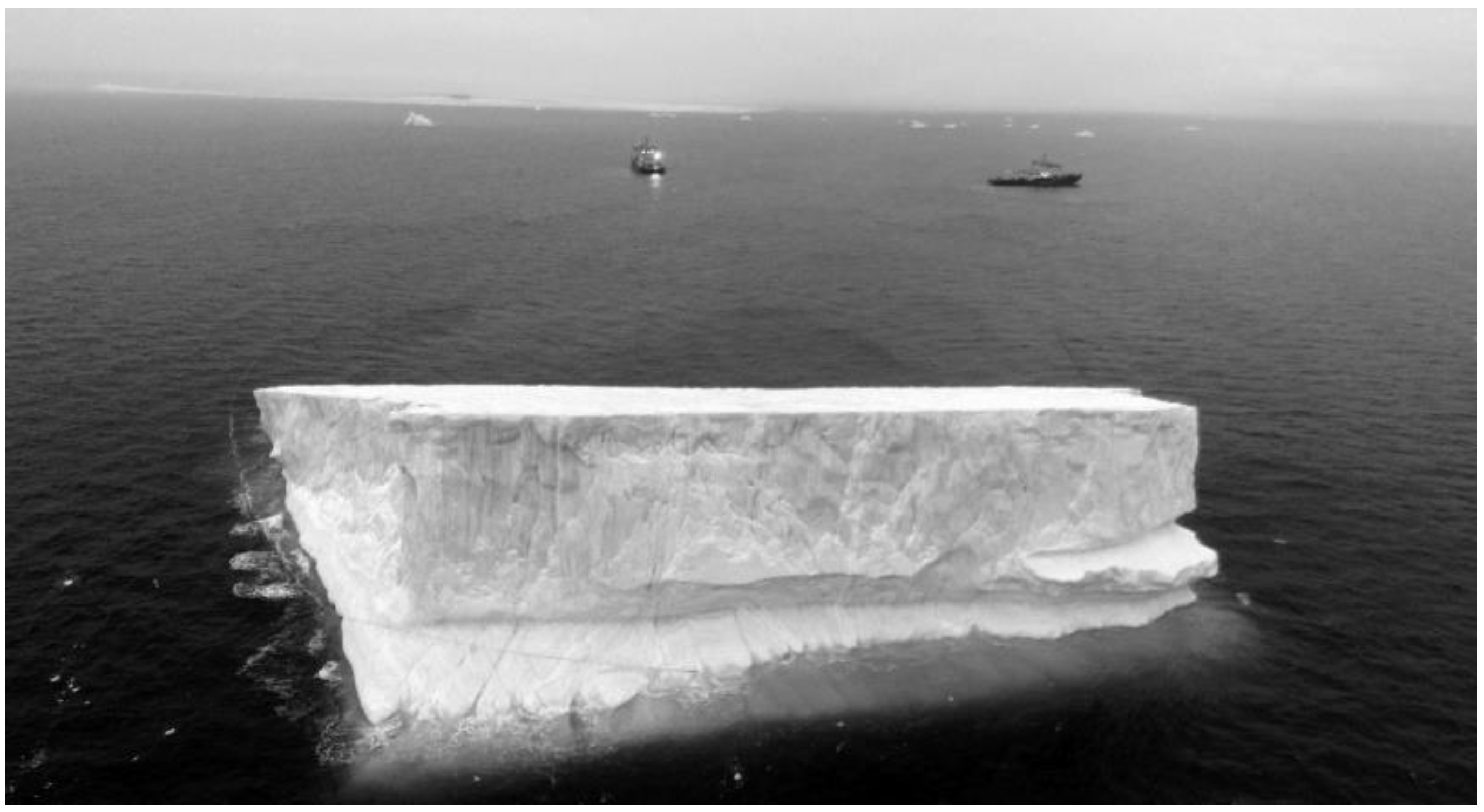
World experience in iceberg transport is gradually increasing. However, it is associated with a slightly different problem: the threat of collision of icebergs with oil rigs. Oil companies in the North and Norwegian seas and off the coast of Newfoundland rent special vessels that hook up dangerous icebergs and change their drift rate by several degrees to avoid collision with the rig [43]. Moreover, these actions should be thoroughly planned and practiced (Figure 1).

Figure 1.
The towing of an over two-million-ton iceberg, using two icebreakers [43].
Attention should be also paid to Sloane’s project (No. 5, Table 1), which considers iceberg towing and mass loss during its transport. This project investigates the transport of icebergs with large dimensions (Table 2) on relatively short routes that pass mainly through the cold waters of the southern part of Atlantic Ocean. It should be noted that Sloane’s assumptions, related to the selected route, were as follows: route length—2000 km, average tow speed—0.9 km/h, time to cover the route—3 months. However, the efficiency of the icebergs’ energy-efficient transport on longer routes should also be further investigated.
A number of studies have paid attention to the issues of ice melting [44,45]. Climate simulations related to ice shelf melt and dynamics of freshwater fluxes across the sea surface were carried out by Gwyther et al. [46], Kimura et al. [47], Liu et al. [48], Lemström et al. [49], Mackie et al. [50], Stouffer et al. [51], and Silva et al. [52]. Paolo et al. [53] highlighted that volume loss from Antarctic ice shelves is accelerating. Eirund et al. [54] paid attention to the effect of airmass perturbations on boundary layer and cloud changes, as well as their impact on the surface radiative balance, especially over sea ice with regard to sea ice melt. The dynamics and trends of sea ice albedo and melt ponds in the Arctic for the years 2002–2011 was analyzed by Istomina et al. [55]. The melt pond fraction and sea ice albedo spatial and temporal dynamics obtained with the Melt Pond Detection retrieval scheme for the Medium Resolution Imaging Spectrometer satellite data were studied. Eicken et al. [56] found that the seasonal evolution of first-year and multiyear ice permeability and surface morphology determine several distinct stages of ice melt. The areas of improvement for fully prognostic simulations of ice albedo have been identified, calling for parameterizations of sea ice permeability and the integration of ice topography and refined ablation schemes into atmosphere–ice–ocean models.
Sivák et al. [57] noted that rain or snow affects heat exchange. Duarte et al. [2] used meteorological data, satellite observations of sea ice concentration and drift to investigate sea ice melt in the analyzed Atlantic water case study. The modeling carried out revealed that realistic melt rates require a combination of warm near-surface Atlantic water and storm-induced ocean mixing. In turn, Carmack et al. [14] made an attempt to summarize the understanding of how heat reaches the ice base from the original sources—inflows of Atlantic and Pacific water, river discharge, and summer sensible heat and shortwave radiative fluxes on the ocean/ice surface—and speculated on how such processes may change in the new Arctic. Sutterley et al. [58] compared four independent estimates of the mass balance of the Amundsen Sea Embayment of West Antarctica, an area experiencing rapid retreat and ice mass loss to the sea. However, it should be noted that these positions mainly describe ice melting in regard to freshwater fluxes across the sea surface, but do not consider the issue of iceberg mass loss during its towing.
An analysis of available literature revealed that the methodology for calculating the mass losses of towed icebergs was not described in detail. Available literature positions include mainly the route simulation results and do not show the way the research can be conducted. Moreover, the are no dependences of iceberg towing speed on the iceberg melt while considering transport conditions. Therefore, an appropriate calculation methodology should be developed.
3. Methodology
3.1. Assumptions of Physical Parameters
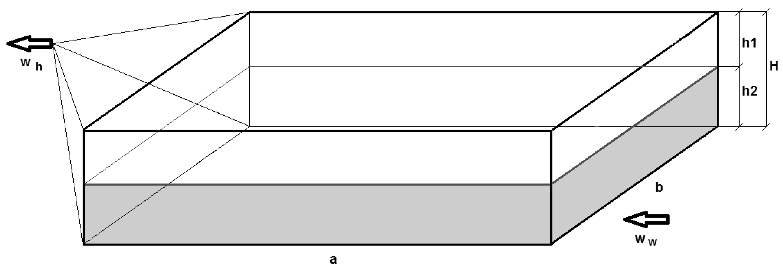
In order to conduct the research, the set of assumptions was determined. Initial calculated iceberg parameters are presented in Figure 2. The index 0 was used to indicate the parameters of the iceberg at the beginning of the route.
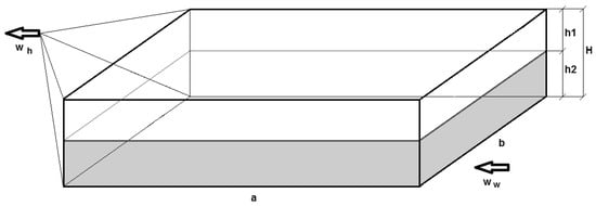
Figure 2.
Iceberg calculation scheme (own elaboration), where: wh—tug speed, ww—current speed, H—total height of the iceberg, h1—height of the above-water part of the iceberg, h2—height of the underwater part of the iceberg (own elaboration).
The most important assumptions related to the movement of the iceberg during its towing include the following:
- That the icebergs are moving using sea currents. This fact allows for the reduction of fuel consumed by the tugs. Due to the significant differences in conditions prevailing at different route sections while the iceberg moves toward its destination [12,59], the concept of calculating the ice losses is adopted individually for every section of the route, and for every season;
- That the iceberg is flowing with the speed V0 using natural currents, the speed increase that the tug needs to use;
- Take into account the large size of the iceberg and its proportion, the heat exchange for all its walls, both above-water and underwater (submerged) surfaces, are treated as flow around the unlimited wall [60,61];
- That the ice surface temperature Tl at all walls is assumed at 0 °C [61], as well as the water temperature at all walls is the same;
- That when the iceberg moves at low speeds, in fixed conditions of heat exchange and is surrounded by water, a laminar boundary layer of freshwater is formed, moving together with the iceberg. At the bottom surface of the iceberg, a zone of permanent thermal stratification is formed [61], where the stratification of water masses, according to their density without their mixing, is observed (in this case, the effect of water salinity on the heat transfer coefficient α can be neglected.). These conditions correspond to low values of this coefficient (α = 20–40 W/m2K), while the current speed has a weak effect on this value. For the vertical iceberg surfaces, the α coefficient depends on the speed of the berg related to the current, the water’s salt content and temperature, and the slope of the surface related to the vertical plane [62]. In sea water with temperatures above 4–8 °C, an ascending stream occurs, while at higher temperatures—a descending stream ensues [61,63].
It should be also noted that the height of the underwater part h2 of the iceberg chosen for transportation is limited by selected conditions. The average value of this parameter should be at least 50 m, which guarantees the stability of the towed iceberg. At the same time, a depth of more than 100 m (even taking into account its decrease during transportation due to melting) can create problems in the port of destination in case the port water area does not have the appropriate depth.
Based on preliminary calculation results and literature data analysis [61], it was also assumed that heat exchange between the air and the above-water part of the iceberg does not have a significant effect on the final result of conducted calculations. When the air temperature is below 0 °C, there is an increase in ice mass and its density due to the condensation of moisture from the air as well as snowfall. When temperatures are above 0 °C, the opposite situation takes place—the ice and snow melt. The melting of the above-water part of the iceberg is not considered in the presented methodology, estimating this at the level of a 5% loss in relation to the initial mass of the underwater part of the iceberg. The calculation methodology also does not take into account the total mass increase for the above-water part of the iceberg under certain weather conditions (outside temperature above 0 °C), considering the pessimistic conditions of iceberg transport. However, the differences in the following conditions of iceberg transport, within individual route sections, are taken into account:
- Weather conditions, especially wind speed influence on the iceberg during particular sections of the route;
- Ice density and, respectively, its mass in the above-water and underwater parts of the iceberg;
- Values of the heat transfer coefficient α, assuming that it is 5–10 times lower for ice–air relation, when compared to coefficient values for ice–water heat exchange.
- Furthermore, the following limitations were set:
- Due to the adopted proportions of iceberg dimensions, the option of the iceberg “tipping over”, as well as iceberg horizontal rotations during towing are not considered;
- The methodology does not take into account the way the iceberg is towed, thus omitting the heat exchange of ropes that the iceberg is towed with;
- Impact of sea waves on transported iceberg is ignored, mainly due to the size of the iceberg, although this can be taken into account by the relative increase in mass loss of about 10–15% [31], which results from the proportion of the surface on which the waves make an impact in relation to the total underwater surface;
- The ability to limit ice–air heat exchange by covering the top with an appropriate screen [28] is not considered.
Based on the abovementioned set of assumptions, the mathematical model was elaborated.
3.2. Mathematical Model
Multi-agent simulation was used to conduct the research. After selecting the route and dividing it into sections, the conditions of iceberg transport within particular sections are analyzed and appropriate calculations are carried out. It is considered that a tug is used while the iceberg is flowing with the current.
The speed of the iceberg wg in relation to the speed of water ww and the speed of the tug wh may be determined on the basis of the vector triangle principle, using the following formulas:
where φ—angle of the route direction relative to the direction of the sea current.
In order to assess the iceberg’s melting speed, the heat transfer coefficient α should be calculated. For the underwater part of the iceberg at low water speed, this coefficient may be calculated using the formula [60]:
where Nu—Nusselt number, Re—Reynolds number, Pr—Prandtl number.
The transformation of this formula to evaluate infinite large surfaces allows for its simplification, as shown below [61]:
where B—proportionality coefficient, λ—water thermal conductivity coefficient at 0 °C, ν—kinematic viscosity of water at the same temperature.
Formula (4) means that, at least within the adopted range of changes in speed and temperatures, the α coefficient for water–ice heat transfer (applied to vertical surfaces [64]) is linearly dependent on the speed of the iceberg in relation to the surrounding water (fresh and sea (saline)). The i index refers to the relevant section of the route (where different climatic conditions may occur), while the j index refers to the relevant iceberg surface (e.g., bottom, side, front, rear).
The values of the iceberg’s mass loss, established for its respective surfaces and for individual sections of the route, can be determined by applying the generalized heat balance equation [60,61,62]:
where V—iceberg’s volume, F—melting surface, r—specific heat of ice melting, τ—time, related to the relevant section of the route and the iceberg’s surface, Tl—temperature of the iceberg’s surface, Tw—temperature of water, identified for the relevant section of the route and the iceberg’s surface.
Assuming the elementary heat exchange surface F for the selected surface of the iceberg and the selected zone, the Formula (6) may be simplified as follows:
where wl—the ice melting speed at the respective surface, expressed in m/s.
The wl value determines the loss of the iceberg’s mass at the end of its transport route. The thickness of the molten ice layer δ in the i-th section of the route, at the j-th wall of the underwater part of the iceberg is calculated as follows:
where τi—the time required to cover the i-th section of the route.
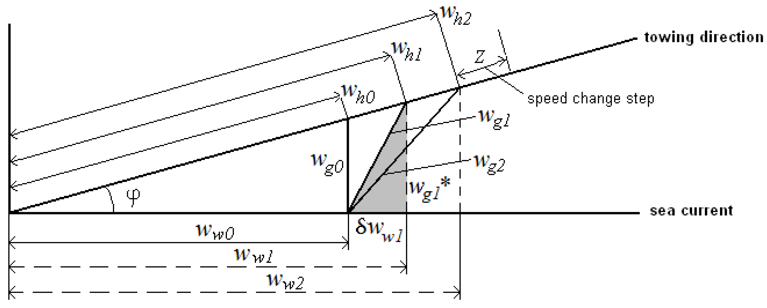
In order to analyze the impact of towing speed on mass loss, the following approach is proposed. It should be noted that by increasing the towing speed, the transport time τ is reduced; however, the intensity of ice melting wl simultaneously increases. The calculation algorithm presented below is illustrated with a diagram in Figure 3. It is assumed that the wh0 value is equivalent to the minimum towing speed, ensuring that the set course is kept, and that the sea current speed wh0, adopted for a respective section of the route, remains unchanged. The adopted water speed, considering an increase of towing speed with step z, may be calculated as follows:
where wh1 = wh0 + z.
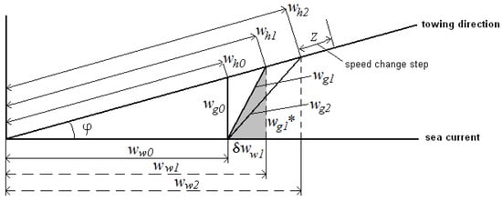
Figure 3.
Vector diagram for calculating the wg value for the selected section of the route (own elaboration).
The adopted increase of this value may be evaluated using the formula:
Therefore:
From the triangle marked in grey in Figure 3, it follows that:
The wg values are calculated analogously for subsequent cycles. Considering the speed increase using the set step z, it is possible to find the speed range that is the most efficient for iceberg’s transport.
The presented methodology was used to develop computational programs. Calculations were conducted using QBASIC i Matlab software. It allowed us to trace the impact of various factors (variables), including towing speed, on the iceberg’s mass loss for selected routes.
4. Results and Discussion
4.1. Case Study Description
The analyzed case study focuses on iceberg-sourced freshwater delivery to Cape Town (South Africa). Cape Town was considered in different projects as a city that needs to be supplied with freshwater [65]. It was also chosen for further analysis due to its location. In the southern part of the Atlantic Ocean, 2000 km away from Cape Town, only single, relatively small icebergs drift, mostly in the November–December period [59]. Their small number strongly limits the selection of icebergs suitable for transport. Therefore, the more remote locations of icebergs were analyzed in the case study.
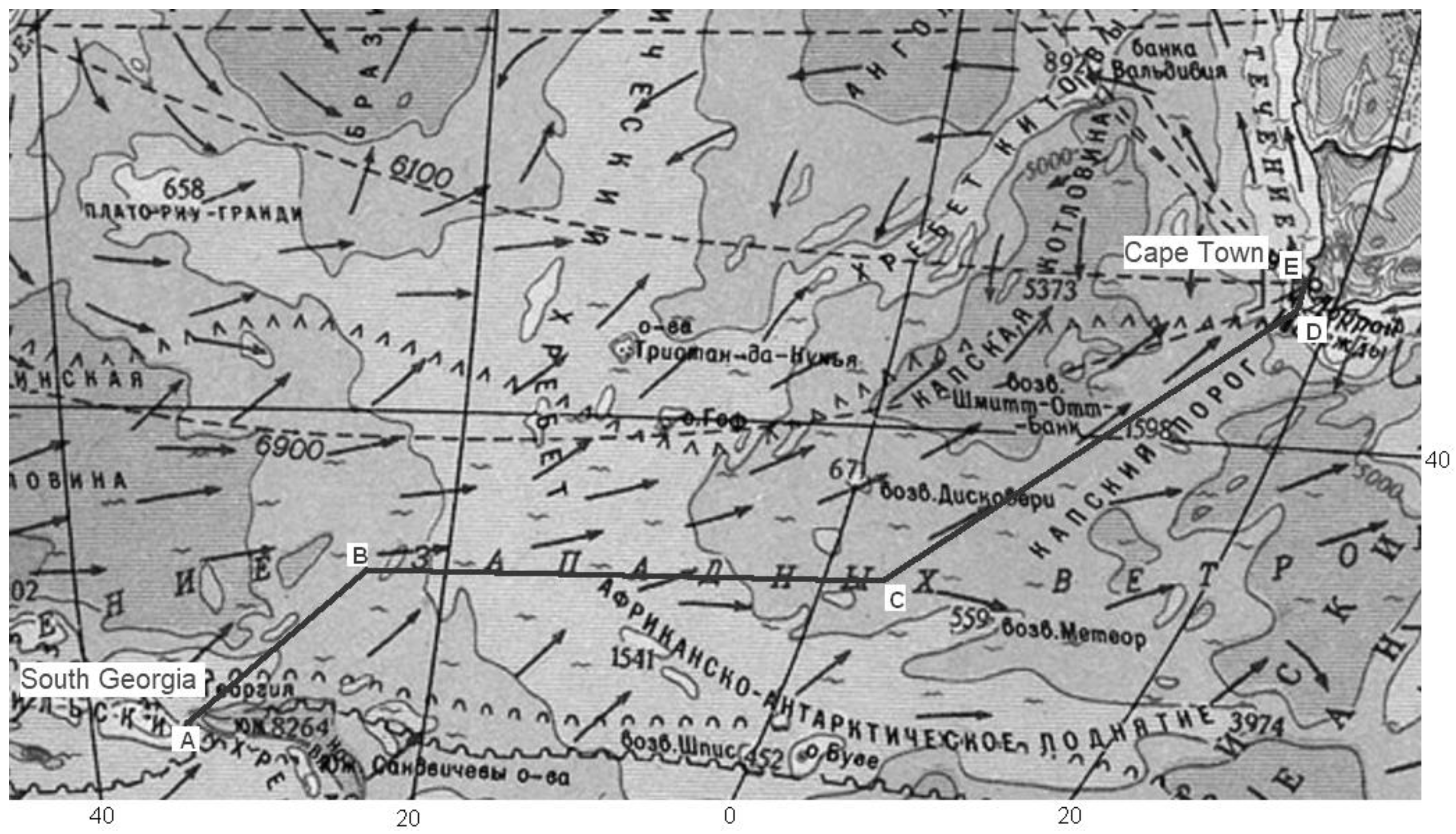
The south-eastern coast of the island of South Georgia was adopted as an area for the iceberg selection (Figure 4). This area was chosen due to the floating icebergs observed there during the August–September period [12]. These icebergs are carried away from the continent by the eddy current of the Weddell Sea, and some of them run aground [66]. The shortest distance from South Georgia to Cape Town is about 4730 km [67]. In the case of an attempt to maximize the use of ocean currents to transport the icebergs, the route extends to about 6100 km (Figure 4, Table 3).

Figure 4.
The sections of selected iceberg transport route (own elaboration based on [59]).
Table 3.
Assumptions for input parameters, divided into route sections considering climate zones (own elaboration).
Selected climate assumptions for the respective sections of the route are presented in Table 3. Taking into account the initial results of transport time calculations, the temperature assumptions for the A–C route sections were adopted for the August–November period, and the C–E sections, for the November–January period.
4.2. Calculation Results
The parameters used to calculate the iceberg’s mass loss on the selected route are presented in Table 4. By substituting the physical values in the Formula (4), the B = 1938 J/m3K was calculated. The differences in heat exchange conditions at the respective iceberg surfaces on the individual walls of the underwater part of the iceberg during particular route sections are presented in Table 5.
Table 4.
Basic parameters used for calculation (own elaboration).
Table 5.
Calculated and assumed average values of the heat transfer coefficient α on the respective walls of the underwater part of the iceberg, W/m2K (own elaboration).
Calculated values of ice melting speed wl and the thickness of the molten layer δ, based on Formula (8) for the respective surfaces and individual sections of the route, are presented in Table 6.
Table 6.
Calculated values of ice melting speed and thickness of molten layer for the respective surfaces and individual sections of the route (own elaboration).
The calculation results of mass loss for the underwater part of the iceberg, for route sections and total route are presented in Table 7. The calculations show the values of the losses at the end of individual route sections.
Table 7.
The calculated mass loss of the underwater part of the iceberg for individual route sections and total route (own elaboration).
Taking into account the set assumptions, the estimated mass losses of iceberg on the selected route are:
- For its underwater part—about 22.5%;
- For its above-water part—about 5%.
The final mass of both parts of the iceberg, transported within the selected route, account for 71.673 and 31.112 million tons, respectively, which correspond to an overall iceberg mass loss of 17.9%. The comparison of the final masses of the above-water and underwater parts clearly indicates that by the end of the journey, the mass of the underwater part of the iceberg remains significantly higher than the mass of the above-water part, which indicates the impossibility of its toppling over and the correctness of the adopted assumptions.
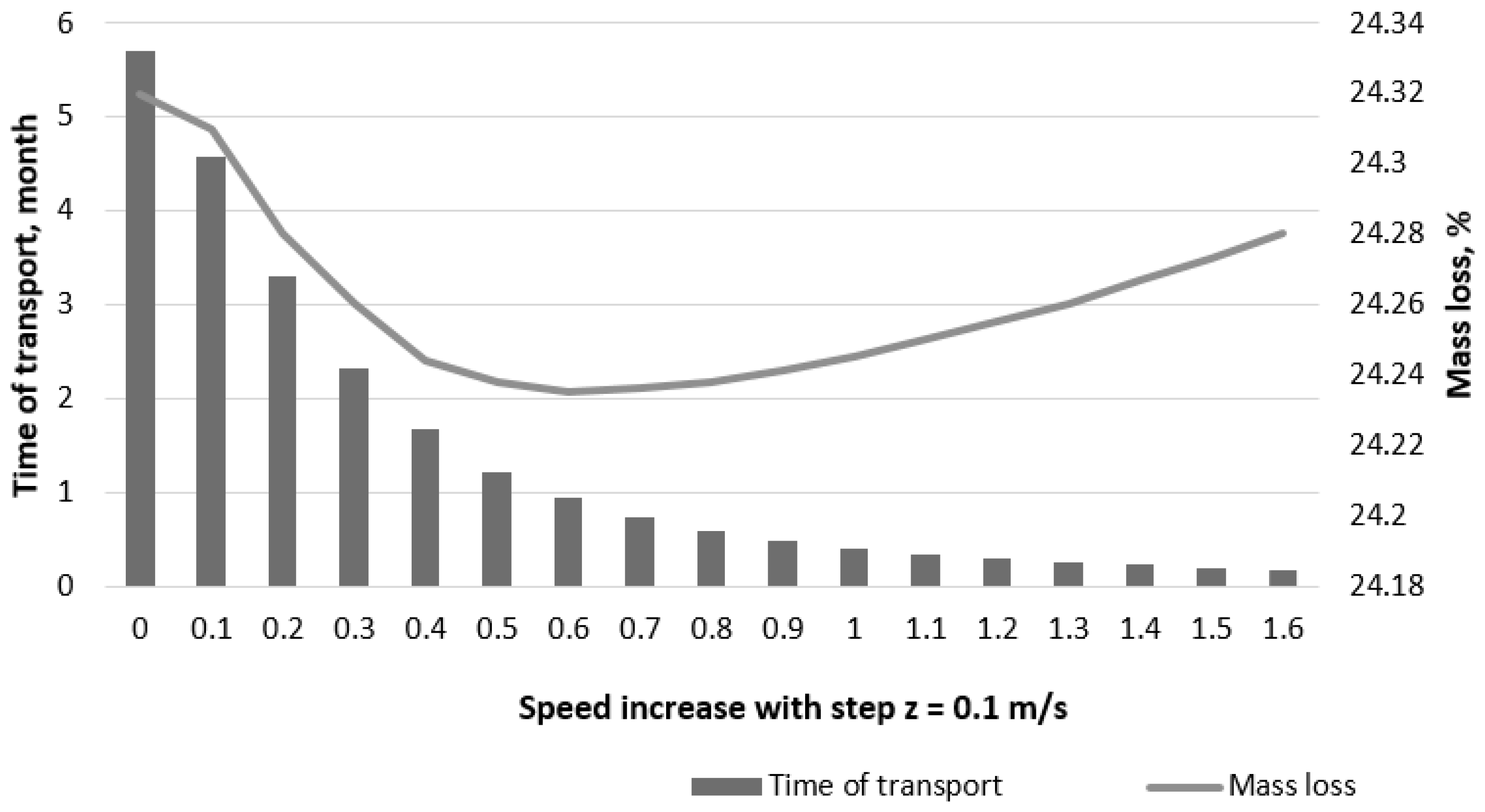
In order to determine the optimal towing speed of the iceberg, we assume that the towing speed increase step z is 0.1 m/s. The subsequent values of this speed relative to water wg for each step were calculated (Figure 5).

Figure 5.
Dependence of route travel time and loss of mass of the underwater part of the iceberg on towing speed (own elaboration).
The results analysis (Figure 5) demonstrates that as long as the heat transfer coefficient α linearly depends on the speed of the iceberg relative to water, the trend of the increase in the ice melting speed wl is balanced by the shorter time required to cover the route. This means that the ice mass loss only minimally depends on the towing speed. The slight variations of ice loss values noticeable in Figure 5 for speed changes are within 0.5%, which is 15–20 times less than the accuracy for calculating the α coefficient. These variations can be explained by a separate analysis of ice losses along the sections of the route and at the walls of the iceberg. Increasing the relative speed of the iceberg over 0.5 m/s (along with increasing the tow speed over 2.0 m/s) leads to the breaking of the laminar layer of cold water at the walls of the iceberg and the need to apply different formulas to calculate the α coefficient for the conditions of forced convection. In turn, this causes the rate of α increase to be significantly greater than the rate of shortening the travel time, thus leading to a significant increase in the iceberg’s mass loss.
Considering that the curve of the dependence of the iceberg’s mass loss on the towing speed has a weakly expressed minimum (Figure 5), a rather wide range of towing speeds wh can be recommended as optimal (from 0.4 to 1.0 m/s). The specific choice for this speed depends on the priorities set by the decision maker. If there is a priority to minimize the travel time, then the speed values closer to the upper bound of the range may be chosen. If the priority is to minimize fuel consumption for tugs, the speed values closer to the lower bound of the wh range may be selected.
The calculation results clearly indicate the desirability for the icebergs’ towing at low speeds. The presented research results do not take into account the possibility of reducing the cost of these tasks by using, for example, a kite adapting to the gusts of the wind, placed over the iceberg on a rope. The use of such and other innovative propulsion systems would reduce fuel consumption by approximately 20–30%.
When analyzing ice losses during towing, some authors of iceberg transport projects (e.g., Georges Mougin [32]) take into account the erosion of the iceberg vertical surface near the water line due to sea (ocean) waves. Undoubtedly, this process is taking place. In Mougin’s project, the initial iceberg mass was 7 million tons; however, in this article, the transport of an iceberg with an assumed mass of 125 million tons was analyzed, which is almost 18 times more. Accordingly, in the example considered in this study, the impact of wave erosion is correspondingly smaller and can be estimated at a level of a small percentage of the total mass loss.
Moreover, breakages of large pieces of iceberg due to emerging cracks may take place during iceberg towing. These phenomena are of random nature and were not taken into account in the presented methodology. Nevertheless, this process can be considered by correction factor implementation. However, its estimation requires a large array of experimental data that are currently unavailable in the literature for the analyzed subject.
However, it should be highlighted that the research results may have been influenced by the assumptions and limitations set solely for the purpose of making calculations. In reality, different weather conditions may take place. The proposed methodology does not take into consideration waves and storms that can influence the icebergs during its towing to its destination [68]. Therefore, the calculation methodology may be improved in order to take these issues into account.
5. Conclusions
The shortage of drinking water is increasing every year and is observed on almost all continents (except Antarctica). It has generated an increased interest in various water supply projects that were previously considered as unrealistic or very difficult to implement. Nowadays, a number of concept projects has been developed, and specialists are trying to solve specific technical problems related to freshwater supply.
The icebergs’ transportation allows for access to high quality water for inhabitants of regions threatened with shortages of freshwater supply. The proposed methodology showed a possible way to assess the mass loss of towed icebergs. The obtained calculation results are reliable, and methodology may be applied to assess the mass loss of icebergs during their energy-efficient towing at low speeds on different routes.
It has been established that the iceberg’s mass loss, calculated for the selected 6103 km long route, was 17.9%. This result may be compared with the assumptions presented in Sloane’s project [36,37,38,39] and other projects. The received calculated value is slightly below the possible iceberg mass loss presented in other projects. It should be noted that Sloane’s project assumed iceberg mass loss at a level of up to 30%, considered for shorter routes, and higher towing speeds; however, iceberg transport time was comparable. The presented calculation results showed that the level of losses may be similar, however, on a longer route selected under set assumptions. On that basis, it may be stated that presented methodology may be widely used to conduct calculations of towed icebergs’ mass loss.
The results of the conducted analysis prove that the correct selection of the route, combined with the maximum use of ocean currents, can prevent additional costly treatments such as insulation of both the underwater and above-water parts of the iceberg, limiting the heat exchange of the iceberg with water during movement.
Moreover, it was possible to calculate the optimal speed range for iceberg transport. For the analyzed case, it was 0.4–1 m/s. Therefore, it could be stated that the minimum loss of ice mass is obtained for towing speeds equivalent to some 1.5 times the average ocean current speed. Low towing speeds, required to keep the set course, may be treated as optimal for the minimization of fuel consumed by the tug. The possibility of iceberg transport for longer distances was also demonstrated. The achieved results may be beneficial for institutions responsible for the development of freshwater supply and the sustainable utilization of water resources.
Our further research will deal with an assessment of the effectiveness of approaches applied to minimize the heat transfer between iceberg and water. The effective ways to use sails on icebergs to increase their transport speed to ports will be considered. Moreover, the technologies to get freshwater from icebergs in ports should be further discussed.
Author Contributions
Conceptualization, S.F.; methodology, S.F., I.S. and L.F.-D.; software, S.F.; validation, L.F.-D.; formal analysis, I.S.; investigation, S.F. and L.F.-D.; resources, I.S. and L.F.-D.; data curation, L.F.-D.; writing—original draft preparation, S.F. and I.S.; writing—review and editing, L.F.-D.; visualization, S.F.; supervision, S.F.; funding acquisition, L.F.-D. All authors have read and agreed to the published version of the manuscript.
Funding
This research was funded by the West Pomeranian University of Technology in Szczecin, Poland. In addition, if accepted, the APCs will be funded by the West Pomeranian University of Technology in Szczecin, Poland.
Institutional Review Board Statement
Not applicable.
Informed Consent Statement
Not applicable.
Data Availability Statement
Not applicable.
Acknowledgments
The authors would like to acknowledge the West Pomeranian University of Technology in Szczecin, Poland for funding this work.
Conflicts of Interest
The authors declare no conflict of interest. The funders had no role in the design of the study; in the collection, analyses, or interpretation of data; in the writing of the manuscript; or in the decision to publish the results.
References
- Jacobs, H.E.; Du Plessis, J.I.; Nel, N.; Gugushe, S.; Levin, S. Baseline adjustment methodology in a shared water savings contract under serious drought conditions. Water SA 2020, 46, 22–29. [Google Scholar] [CrossRef] [Green Version]
- Duarte, P.; Sundfjord, A.; Meyer, A.; Hudson, S.R.; Spreen, G.; Smedsrud, L.H. Warm Atlantic Water explains observed sea ice melt rates north of Svalbard. J. Geophys. Res. Oceans 2020, 125, e2019JC015662. [Google Scholar] [CrossRef]
- Brown, C.; Lall, U. Water and economic development: The role of inter annual variability and a framework for resilience. Nat. Resour. Forum 2006, 30, 306–317. [Google Scholar] [CrossRef]
- The Food and Agriculture Organization. Climate Change, Water and Food Security; The Food and Agriculture Organization: Rome, Italy, 2011; 176p. [Google Scholar]
- Goga, T.; Friedrich, E.; Buckley, C.A. Environmental life cycle assessment for potable water production—A case study of seawater desalination and mine-water reclamation in South Africa. Water SA 2019, 45, 700–709. [Google Scholar] [CrossRef] [Green Version]
- Kirby, T. Stephen Luby: Promoting the importance of water for health. Lancet 2009, 374, 1961. [Google Scholar] [CrossRef]
- Shomar, B. Water Resources, Water Quality and Human Health in Regions of Extreme Stress. Middle East. J. Earth Sci. Clim. Chang. 2013, 4, 153. [Google Scholar] [CrossRef] [Green Version]
- Berke, J. An Engineering Firm Wants to Tow Icebergs Thousands of Miles from Antarctica to Quench the Driest Areas of the World—And It’s Starting with Dubai. Business Inside. 2018. Available online: http://www.businessinsider.com/engineering-firm-tow-icebergs-antarctica-for-water?IR=T.html (accessed on 20 November 2020).
- World Health Organization/UNICEF. Wash in Health Care Facilities; Global Baseline Report 2019; World Health Organization/UNICEF: Geneva, Switzerland, 2019. [Google Scholar]
- Dinniman, M.; Asay-Davis, X.; Galton-Fenzi, B.; Holland, P.; Jenkins, A.; Timmermann, R. Modeling ice shelf/ocean interaction in Antarctica: A review. Oceanography 2016, 29, 144–153. [Google Scholar] [CrossRef] [Green Version]
- Duan, C.; Dong, S.; Wang, Z.; Liao, Z. Climatic characteristics of drift ice in the northern Barents Sea. J. Water Clim. Chang. 2020, 11, 800–811. [Google Scholar] [CrossRef]
- Kholoptsev, A. Changes in the temperature of surface currents in the southern hemisphere of the Earth, which are part of the global thermal oceanic conveyor during modern climate warming. Meteorological 2012, 14, 104–113. (In Russian) [Google Scholar]
- Orheim, O. The polar oceans and climate change. In the World Ocean in Globalisation: Climate Change, Sustainable Fisheries, Biodiversity, Shipping, Regional Issues; Brill Nijhoff: Leiden, The Netherlands, 2011; pp. 147–154. [Google Scholar] [CrossRef]
- Carmack, E.; Polyakov, I.; Padman, L.; Fer, I.; Hunke, E.; Hutchings, J.; Jackson, J.; Kelley, D.; Kwok, R.; Layton, C.; et al. Toward quantifying the increasing role of oceanic heat in sea ice loss in the new Arctic. Bull. Am. Meteorol. Soc. 2015, 96, 2079–2105. [Google Scholar] [CrossRef]
- Zakhvatkina, N.; Smirnov, V.; Bychkova, I. Satellite SAR data-based sea ice classification: An overview. Geosciences 2019, 9, 152. [Google Scholar] [CrossRef] [Green Version]
- Tournadre, J.; Bouhier, N.; Girard-Ardhuin, F.; Rémy, F. Large icebergs characteristics from altimeter waveforms analysis. J. Geophys. Res. Oceans 2015, 120, 1954–1974. [Google Scholar] [CrossRef]
- Gwyther, D.E.; Galton-Fenzi, B.K.; Dinniman, M.S.; Roberts, J.L.; Hunter, J.R. The effect of basal friction on melting and freezing in ice shelf-ocean models. Ocean Model. 2015, 95, 38–52. [Google Scholar] [CrossRef]
- Lund, B.; Graber, H.C.; Pog, P.; Smith, M.; Doble, M.; Thomson, J.; Wadhams, P. Arctic sea ice drift measured by shipboard marine radar. J. Geophys. Res. Oceans 2018, 123, 4298–4321. [Google Scholar] [CrossRef]
- McKenna, R.; Loewen, A.; Crocker, G. A finite element model for the deformation of floating ice covers. Cold Reg. Sci. Technol. 2021, 182, 103213. [Google Scholar] [CrossRef]
- Girard-Ardhuin, F.; Ezraty, R. Enhanced arctic sea ice drift estimation merging radiometer and scatterometer data. IEEE Trans. Geosci. Remote Sens. 2012, 50, 2639–2648. [Google Scholar] [CrossRef] [Green Version]
- Mäkynen, M.; Haapala, J.; Aulicino, G.; Balan-Sarojini, B.; Balmaseda, M.; Gegiuc, A.; Girard-Ardhuin, F.; Hendricks, S.; Heygster, G.; Istomina, L.; et al. Satellite observations for detecting and forecasting sea-ice conditions: A summary of advances made in the SPICES Project by the EU’s Horizon 2020 Programme. Remote Sens. 2020, 12, 1214. [Google Scholar] [CrossRef] [Green Version]
- Wadhams, P.; Kristensen, M.; Orheim, O. The response of Antarctic icebergs to ocean waves. J. Geophys. Res. 1983, 88, 6053–6065. [Google Scholar] [CrossRef]
- Wadhams, P.; Aulicino, G.; Parmiggiani, F.; Pog, P.; Holt, B. Pancake ice thickness mapping in the Beaufort Sea from wave dispersion observed in SAR imagery. J. Geophys. Res. Oceans 2018, 123, 2213–2237. [Google Scholar] [CrossRef]
- Marson, J.M.; Myers, P.G.; Hu, X.; Le Sommer, J. Using vertically integrated ocean fields to characterize Greenland icebergs’ distribution and lifetime. Geophys. Res. Lett. 2018, 45, 4208–4217. [Google Scholar] [CrossRef]
- Prieto, M. Equity vs. efficiency and the human right to water. Water 2021, 13, 278. [Google Scholar] [CrossRef]
- Peña-Ramos, J.A.; De Luis, F.R. Past, Present, and Future Conflicts over Freshwater. Int. J. Environ. Sustain. 2021, 17, 19–31. [Google Scholar] [CrossRef]
- Filin, S.; Semenov, I.; Filina-Dawidowicz, L. Technical and economic aspects of transporting icebergs to regions threatened with shortages of freshwater supplies. In Proceedings of the 37th IBIMA International Conference, Cordoba, Spain, 1–2 April 2021. [Google Scholar]
- Korzun, V.A. Assessment of the Possibilities of Using Antarctic Resources; IMEMO RAN: Moscow, Russia, 2009; 116p. (In Russian) [Google Scholar]
- Shlionskaya, I. Living Water Can Be Obtained from Icebergs. 2008. Available online: https://www.pravda.ru/science/294541-ice/ (accessed on 17 August 2020). (In Russian).
- The Problem of Fresh Water Supply Has Been Resolved. 2013. Available online: http://korabley.net/news/problema_dostavki_presnoj_vody_reshena/2013-03-25-1410 (accessed on 15 August 2020). (In Russian).
- Ruiz, R. Media Environments: Icebergs/Screens/History. J. North. Stud. 2015, 9, 33–50. [Google Scholar]
- Mamontov, D. Georges Mougins’ Ice Dream: An Iceberg. Pop. Mech. 2012, 2, 12–18. (In Russian) [Google Scholar]
- Bikmurzina, E. Get the Iceberg. Sci. Focus. 2012, 2. Available online: http://www.vokrugsveta.ru/nauka/article/155129/ (accessed on 18 August 2020). (In Russian).
- Alive Water from Antarctica. The Global Ecological Project “ALIVE WATER”—New Technologies of Drinking Water and Cool Air Obtaining from the High-Latitude Ice. 2020. Available online: http://www.khalidov.net/english/water/alivewater_e.html (accessed on 5 August 2020).
- Khalidov, G.; Khalidov, U. Trimaran Ice Carrier. Patent No. RU 2177429 C2, 27 December 2001. [Google Scholar]
- An Iceberg Will Be Shipped from Antarctica to Africa to Water 4 Million People. 2019. Available online: https://lenta.ua/iz-antarktiki-v-afriku-perepravyat-aysberg-chtoby-napoit-4-milliona-lyudey-15635/ (accessed on 12 October 2020). (In Russian).
- A South African Engineer Suggests Supplying Drought-Stricken Cape Town with Water from Icebergs. 2018. Available online: https://densegodnya.ru/nauka/article_post/inzhener-iz-yuar-predlagayet-obespechivat-stradayushchiy-ot-zasukhi-keyptaun-vodoy-iz-aysbergov (accessed on 2 October 2020). (In Russian).
- Heiberg, T. Icebergs Could Float to the Rescue of Cape Town Water Crisis. Reuters. 2018. Available online: https://www.reuters.com/article/us-safrica-drought-iceberg/icebergs-could-float-to-the-rescue-of-cape-town-water-crisis-idUSKBN1I11NF (accessed on 17 September 2020).
- Iceberg Could Solve Cape Town’s Fresh Water Problem. 2018. Available online: https://www.japantimes.co.jp/ (accessed on 16 October 2020).
- Maeno, N. Science of Ice; Hokkaido University Press: Sapporo, Japan, 1981; 240p. [Google Scholar]
- Filin, S.; Semenov, I. Innovative technologies for the use of ice-composite materials in the construction and operation of floating objects. Refrig. Bus. 2011, 7, 22–29. (In Russian) [Google Scholar]
- Filin, S.; Semenov, I. The use of ice and ice composites in shipbuilding and water tourism. Tech. chłodnicza Klim. 2011, 9, 426–432. (In Polish) [Google Scholar]
- OOO “Gazprom geologorazvedka” Conducted an Exercise in the Kara Sea. 2018. Available online: http://www.gazprom.ru/press/media/2018/833245/ (accessed on 11 September 2020). (In Russian).
- Li, Y.; Yan, Z.; Yang, C.; Guo, B.; Yuan, H.; Zhao, J.; Mei, N. Study of a Coil Heat Exchanger with an Ice Storage System. Energies 2017, 10, 1982. [Google Scholar] [CrossRef] [Green Version]
- Dinniman, M.S.; Klinck, J.M.; Smith, W.O. Influence of sea ice cover and icebergs on circulation and water mass formation in a numerical circulation model of the Ross Sea. Antarctica. J. Geophys. Res. 2007, 112, C11013. [Google Scholar] [CrossRef] [Green Version]
- Gwyther, D.E.; Kusahara, K.; Asay-Davis, X.S.; Dinniman, M.S.; Galton-Fenzi, B.K. Vertical processes and resolution impact ice shelf basal melting: A multi-model study. Ocean Model. 2020, 147, 101569. [Google Scholar] [CrossRef]
- Kimura, S.; Nicholls, K.W.; Venables, E. Estimation of ice shelf melt rate in the presence of a thermohaline staircase. J. Phys. Oceanogr. 2015, 45, 133–148. [Google Scholar] [CrossRef] [Green Version]
- Liu, Y.; Moore, J.C.; Cheng, X.; Gladstone, R.M.; Bassis, J.N.; Liu, H.; Wen, J.; Hui, F. Ocean-driven thinning enhances iceberg calving and retreat of Antarctic ice shelves. Proc. Natl. Acad. Sci. USA 2015, 112, 3263–3268. [Google Scholar] [CrossRef] [Green Version]
- Lemström, I.; Polojärvi, A.; Tuhkuri, J. Numerical experiments on ice-structure interaction in shallow water. Cold Reg. Sci. Technol. 2020, 176, 103088. [Google Scholar] [CrossRef]
- Mackie, S.; Smith, I.J.; Ridley, J.K.; Stevens, D.P.; Langhorne, P.J. Climate response to increasing Antarctic iceberg and ice shelf melt. J. Clim. 2020, 33, 8917–8938. [Google Scholar] [CrossRef]
- Stouffer, R.J.; Seidov, D.; Haupt, B.J. Climate response to external sources of freshwater: North Atlantic versus the Southern Ocean. J. Clim. 2007, 20, 436–448. [Google Scholar] [CrossRef] [Green Version]
- Silva, T.A.M.; Bigg, G.R.; Nicholls, K.W. Contribution of giant icebergs to the Southern Ocean freshwater flux. J. Geophys. Res. Oceans 2006, 111, C03004. [Google Scholar] [CrossRef]
- Paolo, F.S.; Fricker, H.A.; Padman, L. Volume loss from Antarctic ice shelves is accelerating. Science 2015, 348, 327–331. [Google Scholar] [CrossRef] [Green Version]
- Eirund, G.K.; Possner, A.; Lohmann, U. The impact of warm and moist airmass perturbations on arctic mixed-phase stratocumulus. J. Clim. 2020, 33, 9615–9628. [Google Scholar] [CrossRef]
- Istomina, L.; Heygster, G.; Huntemann, M.; Marks, H.; Melsheimer, C.; Zege, E.; Malinka, A.; Prikhach, A.; Katsev, I. Melt pond fraction and spectral sea ice albedo retrieval from MERIS data—Part 2: Case studies and trends of sea ice albedo and melt ponds in the Arctic for years 2002–2011. Cryosphere 2015, 9, 1567–1578. [Google Scholar] [CrossRef] [Green Version]
- Eicken, H.; Krouse, H.R.; Kadko, D.; Perovich, D.K. Tracer studies of pathways and rates of meltwater transport through Arctic summer sea ice. J. Geophys. Res. Oceans 2002, 107. [Google Scholar] [CrossRef] [Green Version]
- Sivák, P.; Tauš, P.; Rybár, R.; Beer, M.; Šimková, Z.; Baník, F.; Zhironkin, S.; Čitbajová, J. Analysis of the Combined Ice Storage (PCM) Heating System Installation with Special Kind of Solar Absorber in an Older House. Energies 2020, 13, 3878. [Google Scholar] [CrossRef]
- Sutterley, T.C.; Velicogna, I.; Rignot, E.; Mouginot, J.; Flament, T.; van Den, B.M.; van Wessem, J.M.; Reijmer, C.H. Mass loss of the Amundsen Sea Embayment of West Antarctica from four independent techniques. Geophys. Res. Lett. 2014, 41, 8421–8428. [Google Scholar] [CrossRef] [Green Version]
- Atlantic Ocean. Physical Map. 2020. Available online: http://geoman.ru/geography/item/f00/s00/e0000691/index.shtml (accessed on 30 August 2020). (In Russian).
- Pekhovich, A.I. Basics of Hydro-Ice Thermic; Energoatomizdat: Leningrad, Russia, 1983; 200p. (In Russian) [Google Scholar]
- Shatalina, I.N. Heat Transfer in the Processes of Freezing and Melting Ice; Energoatomizdat: Leningrad, Russia, 1990; 120p. (In Russian) [Google Scholar]
- Carey, V.; Gebhart, B. Transport near a vertical ice surface melting in saline water: Experiments at low salinities. J. Fluid Mech. 1982, 117, 403–423. [Google Scholar] [CrossRef]
- Bobkov, V.A. Ice Production and Application; Food Industry: Moscow, Russia, 1977; 232p. (In Russian) [Google Scholar]
- Gogolev, E.S.; Krasavin, A.N. Influence of the orientation of the ice surface on the intensity of heat transfer from water to ice under conditions of free convection. J. Eng. Phys. Thermoph. 1984, XLVI, 447–451. (In Russian) [Google Scholar]
- Lubofsky, E. Can Icebergs Be Towed to Water-Starved Cities? Wood Hole Oceanographic Institution. 2021. Available online: https://www.whoi.edu/news-insights/content/can-icebergs-be-towed-to-water-starved-cities/ (accessed on 20 June 2021).
- Romanov, A.A. Ice conditions for Navigation in the Southern Ocean. World Meteorological Organization. Mar. Meteorol. Relat. Oceanogr. Act. 1996, 35, 116–119. (In Russian) [Google Scholar]
- Great World Atlas; Pascal: Bielsko-Biała, Poland, 2007; 340p. (In Polish)
- Zhang, Y.; Chen, C.; Beardsley, R.C.; Perrie, W.; Gao, G.; Zhang, Y.; Qi, J.; Lin, H. Applications of an unstructured grid surface wave model (FVCOM-SWAVE) to the Arctic Ocean: The interaction between ocean waves and sea ice. Ocean Model. 2020, 145, 101532. [Google Scholar] [CrossRef]
Publisher’s Note: MDPI stays neutral with regard to jurisdictional claims in published maps and institutional affiliations. |
© 2021 by the authors. Licensee MDPI, Basel, Switzerland. This article is an open access article distributed under the terms and conditions of the Creative Commons Attribution (CC BY) license (https://creativecommons.org/licenses/by/4.0/).