Abstract
The subject of this study is the chemical composition of potentially geothermal waters of the Mesozoic basement of the central part of the Carpathian Foredeep and the Outer Carpathians regions. The research objectives were: (1) to identify statistically significant differences between the chemical composition of waters from the Cretaceous, Jurassic, and Triassic aquifers, and between the waters of both regions; and (2) the discovery of zones indicating active water exchange—attractive due to the operational efficiency of wells. Knowledge of the chemical composition of water allows for the preliminary identification of areas of interest for the exploitation of water for recreational, healing, and heating purposes. The research methods used were: (1) statistical tests and (2) methods of multivariate data analysis, such as the Kruskal–Wallis test and Principal Component Analysis (PCA). The performed tests and statistical analyses allowed us to draw conclusions about significant differences between the chemical composition of waters from the Cretaceous, Jurassic, and Triassic aquifers, and the basement of the Carpathian Foredeep and the Outer Carpathians. They indicated the existence of a zone with symptoms of active water exchange. Before establishing the fact of active exchange of waters in this zone, further research should be undertaken.
1. Introduction
The chemical composition of geothermal waters and, in a broader sense, groundwater is of interest to hydrogeologists, oil geologists, geothermists, heat engineers, and entrepreneurs for many reasons, including:
- Management of groundwater reservoirs for drinking purposes [1];
- Searching in the water the symptoms of neighborhood of hydrocarbon deposits [2];
- Determination of water corrosivity in relation to materials from which the geothermal well infrastructure is made (high concentrations of Cl−, H2S) and scalling phenomena [3,4];
- The ability to recover water components (I, Br, Li, Mg, K, and others) [5];
- Determination of the healing nature of waters for use in spas (e.g., the presence of I, F, H2SiO3) [6,7,8,9];
- Scientific curiosity, and searching for connections between the chemical composition of waters and the environment of their occurrence [10,11,12].
The chemical composition can have a diagnostic role for many phenomena occurring in the rock mass. It can also testify to the conditions of water exchange (active, difficult, and water flow) [13,14]. It can contribute to or impede the optimal exploitation of geothermal water for different purposes, such as recreation and balneotherapy and district heating. Recreational purposes require waters with mineralization of up to 35 g/L, and therapeutic purposes up to 50 g/L [15,16]. In both cases, it is imperative that the waters have a chemical composition suitable for human contact. District heating cells place emphasis on the amount of water stream per time unit during exploitation from the borehole (borehole capacity). A favorable chemical composition of the waters, so as not to cause corrosion and precipitation, is also desirable.
Active water exchange zones may be attractive zones from the point of view of geothermal water exploitation for recreational and therapeutic purposes. From the point of view of heating applications, they may also be promising. The reason for this is the supposition that the conditions in such zones are related to the very good reservoir properties of the rocks. These, in turn, increase the possibility of achieving a high efficiency of the boreholes during operation.
However, the chemical composition of groundwater depends on many coexisting factors [12,13,14,15,16,17,18]. Due to the overlapping nature of these factors, it is not always easy to interpret the chemical composition of water and its origin. Its diagnostic role should be verified, taking into account the many different factors influencing the observed chemical composition.
The central part of the Carpathian Foredeep and the Outer Carpathians were the subjects of a study, specifically the hydrocarbon deposits (e.g., the Grobla–Pławowice and Mniszów deposits), curative waters (Busko–Zdrój and Solec–Zdrój deposits), and the geothermal activity (Cudzynowice GT-1, Busko C-1) [19,20,21,22,23,24,25]. This area has been partially explored by drilling, and therefore is an excellent field for undertaking statistical analysis. A large number of water samples (268 analyzed) allowed for certain calculations and conclusions based on the results. However, since these were not samples taken from randomly selected locations, the conclusions obtained cannot be generalized for groundwater in other areas. The conclusions of the analyses therefore apply only to the geothermal potential of the water of this area.
Some authors have already described selected aspects of the chemical composition of groundwaters in the discussed area and its neighboring areas with commonly used methods of hydrochemical analysis [22,23,24,25,26,27,28,29,30,31,32,33,34,35,36,37,38,39,40,41,42,43,44,45,46].
The author of this article was interested in the chemical composition of groundwater from the Mesozoic formations of the basement of the central part of the Outer Carpathians and the Carpathian Foredeep. These formations collect potentially geothermal waters that have been tested in the drilling of deep boreholes. Water samples were subjected to analysis in order to determine their chemical composition. The chemical analyses used in this study were based on archival data. The water temperature presented here was not measured; therefore, this article refers to ‘potentially geothermal’ waters. Their nature was assessed by the author as “potentially geothermal” on the basis of calculations of the depth temperature (discussed in Section 2.2).
The main goals of this article were:
- To show the chemical composition of the groundwater, which was potentially geothermal, from the Mesozoic formations of the basement of the central part of the Carpathian Foredeep and the basement of the Outer Carpathians;
- To indicate the differences in the chemical composition of waters, divided into groups by: (1) their origin from Cretaceous, Jurassic, or Triassic formations; (2) the origin of the basement of the Carpathian Foredeep or the basement of the Outer Carpathians; and (3) the depth of their occurrence;
- To find zones of interest due to the distinctive chemical composition of the waters, indicating a potentially active water exchange.
These objectives were analyzed using statistical analyses, which gave us answers to the questions presented in Section 2.3.
The author used various statistical tests (tests of normality of distribution, tests of consistency of distribution, tests of homogeneity of variance, tests of independence χ2) and multivariate analyses (Kruskal–Wallis test, non-parametric version of the one-way ANOVA, Duncan’s post hoc tests (Section 3.1)), and Principal Component Analysis (PCA) (Section 3.2).
2. Materials and Methods
2.1. Research Area
The analyzed area was within the borders of Poland (Central-Eastern Europe) (Figure 1).
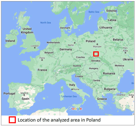
Figure 1.
Location of the analyzed area in Poland on the background of the map of Europe (source: Google Maps).
The subject of the description and statistical analyses presented in this article are the results of water sampling of the Cretaceous, Jurassic, and Triassic aquifers of the Miechów Trough (a part of the Polish Lowlands), submerged under the central part of the Miocene formations of the Carpathian Foredeep and the Flysch formations of the Outer Carpathians. The location of the boreholes from which the water samples were obtained is shown on the map (Figure 2).
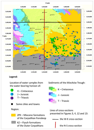
Figure 2.
Distribution of water samples with the described chemical analyses in the analyzed area in Poland, grouped by the Cretaceous (K), Jurassic (J), and Triassic (T) aquifers on the background of the geological map.
Figure 3a,b shows the cross-sections of W–E, and Figure 4a,b shows the cross-sections of N–S along the lines in Figure 2. The first of the cross-sections (Figure 3a and Figure 4a) shows the depth of the middle of the depth interval from which the water samples were taken (the basement of the Carpathian Foredeep and the basement of the Outer Carpathian). The samples from the water-bearing horizon of the Creatceous (K), Jurassic (J), and Triassic (T) aquifers are distinguished in terms of color. The second cross-section (Figure 3b and Figure 4b) shows the distribution of the estimated depth temperatures (Tz), calculated by means of the geothermal gradient (explanation in Section 2.2). The depth shown on the vertical scale in the sections (Figure 3a,b and Figure 4a,b) was exceeded by 20 times, and expressed in m a.s.l (meters above sea level) as opposed to the depth (Z) given in m b.g.l. (meters below ground level).
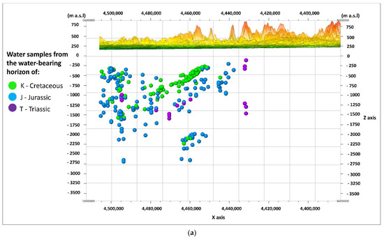
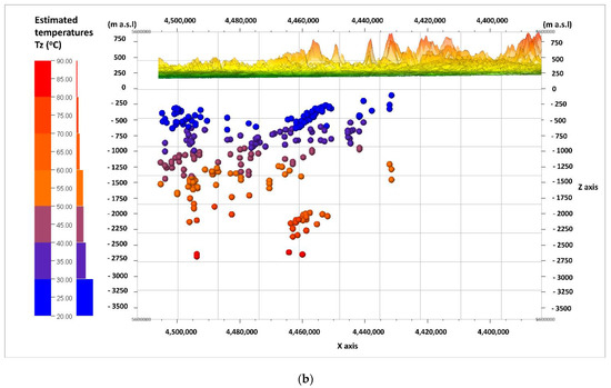
Figure 3.
W–E cross-sections through the analyzed area; view from N, showing: (a) the division of water samples according to their origin from the Cretaceous (K), Jurassic (J), or Triassic (T) aquifers; (b) the distribution of the estimated depth temperatures (Tz).
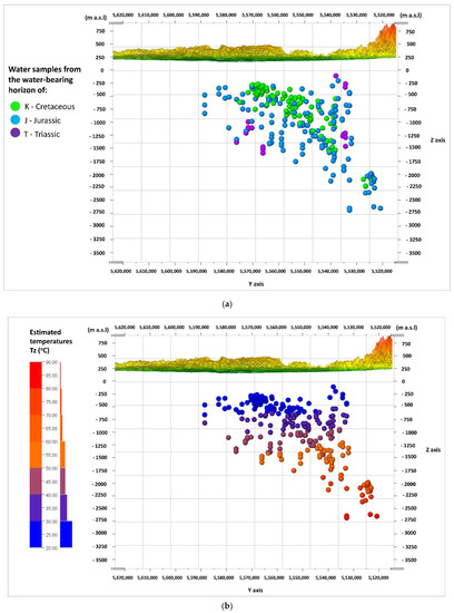
Figure 4.
N–S cross-sections through the analyzed area; view from W, showing: (a) the division of water samples according to their origin from the Cretaceous (K), Jurassic (J), or Triassic (T) aquifers; (b) the distribution of the estimated depth temperatures (Tz).
The arrangement of the Mesozoic formations in the shape of a trough is visible (Figure 3a). It is filled with sediments of the Cretaceous (K) aquifer, and lined with sediments of the Jurassic (J) aquifer. Sediments of the Triassic (T) aquifer have a limited reach in this part of the basin. The estimated (predicted) depth temperatures have the highest values in the deepest parts of the axial part of the basin, in the formations of the Jurassic (J) aquifer, at depths of –2500 to –2750 m a.s.l. Most samples came from the depths, where the expected temperatures do not exceed 60 °C (Figure 3b).
2.2. Characteristics of the Analyzed Data
Out of the 268 results of the chemical analyses of the water samples, 219 results for waters from the basement of the Carpathian Foredeep and 49 results for waters from the basemenst of the Outer Carpathians were used to carry out further statistical analyses. The most numerous results came from the Jurassic (J, 148) and Cretaceous (K, 101) aquifers. These were mostly Cl-Na waters (228 results). The largest number of samples were from depth interval between 500 and 1000 m b.g.l. (123 results). The results of the chemical analyses were relatively evenly divided into the values of TDS (usually 41–56 results each). On the other hand, the most frequently represented values of estimated temperatures (Tz) were in the range of 20–30 °C (98 results).
Table 1 presents the number of the described chemical analyses, grouped by:

Table 1.
The number and percentage of chemical analyses grouped by water-bearing horizon, region, chemical type, depth interval, TDS interval, and estimated depth temperature.
- Water-bearing horizon (Cretaceous—K, Jurassic—J, and Triassic—T);
- Region (the basement of the Carpathian Foredeep—ZPK, the basement of the Outer Carpathians—KZ);
- Chemical type of the water (explanation below);
- Water sampling depth interval (every 500 m);
- Water TDS interval (every 25 g/dm3);
- Estimated temperatures at the depth of water sampling (every 20 °C).
The information contained in the above data and subjected to further statistical analysis included:
- Depth (Z) (in m b.g.l.);
- Density of the water samples (in kg/L);
- TDS of the water samples (in g/L);
- Major ion concentrations (HCO3−, SO42−, Cl−, Ca2+, Mg2+, Na+) (in g/L);
- Concentration of metasilicic acid (H2SiO3) (in g/L);
- Values of hydrochemical indices rNa+/rCl−, rSO42− × 100/rCl−, rHCO3−/rCl−;
- Geothermal gradient Gt (in °C/100 m);
- Estimated temperatures (Tz) (in °C).
Depth (Z) is here defined as the center of the depth interval from which the groundwater sample was taken. Therefore, it is a conventional water abstraction depth.
The temperature (Tz) determined at the depth (Z) is defined as the temperature calculated for the purposes of this article using the geothermal gradient map made by Hajto (2006–2012) [47,48,49]. It was prepared in order to assess the temperatures in the depths of the following areas: Polish Lowlands, Outer Carpathians, and Carpathian Foredeep.
The formula according to the calculated temperature (Tz) at depth (Z) has the following form:
The phenomenon of water cooling during operation was ignored. It causes the temperature of the outflow waters to be lower than the temperature of the waters in the reservoir. Therefore, for these reasons, the waters in question should be considered ‘potentially geothermal’, as their temperatures in the reservoir and at the outflow have not been documented.
In order to determine the chemical type of water from the discussed chemical analyses, the concentrations of individual components, expressed in g/L, were converted to mval/L and % mval anions and % mval cations. Then, we checked which anions and cations exceed the threshold of 20 ± 3% mval anions and 20 ± 3% mval cations. From these, waters were selected in which there was one anion exceeding the required percentage threshold. In waters meeting this criterion, attention was paid to the dominant cation. When creating a name for the “chemical type”, the first member indicated the anion, and the second member indicated the cation. In this way, the following “simple chemical types” were designated in the discussed data: Cl-Na, SO4-Ca, and SO4-Na. One “chemical type” was made up of waters containing one and the same dominant anion, as well as one and the same dominant cation.
If there were two dominant anions among the anions, then cations in the term “type” were not taken into account; rather, only those dominant anions. In this way, the “mixed chemical types” were designated: SO4-HCO3, Cl-HCO3, and Cl-SO4. In the nomenclature of “simple and mixed types”, the order of the dominant anions and cations was not taken into account. This was a simplification of the Altowski-Szwiec classification [50], known and often used in hydrogeology. In it, however, the name of the water begins with the ion whose concentration in the water is the highest, regardless of whether it is an anion or a cation [16]. It generates a much greater variety of “chemical types”, which often makes it difficult to illustrate water chemistry in regional and review studies.
From among the range of hydrochemical indices that can be calculated, the water metamorphism index, rNa+/rCl−, water sulphate index, rSO42− × 100/rCl−, and the bicarbonate-chloride index, rHCO3−/rCl−, were selected as those whose high values may indicate the conditions of active water exchange. However, they do not necessarily indicate the existence of conditions for active exchange (see Section 4), but may be a symptom of it.
Table 2 presents statistical measures for the set of analyzed data (Parameters), which are measures of position and variability. These include: minimum value, first quartile, median, mean, third quartile, maximum value, value range, variance, and standard deviation.
Table 2.
Basic statistical measures for the analyzed data.
The analyzed waters were therefore groundwater from the depth (Z) from 436 to 3077 m b.g.l. Their TDS ranged from 2 to 176 g/dm3, and the estimated temperatures (Tz) in the rock mass at depth (Z) were in the range from 20 to 90 °C.
As is seen on the Piper diagram (Figure 5) most water samples is characterized by Cl− concentration above 60% meq of anions, SO42− concentration below 40% meq of anions and HCO3− concentration below 10% meq of anions, Ca2+ concentration below 40% meq of cations, Na+ concentration above 60% meq of cations and Mg2+ concentration above 80% meq of cations. However, some of the samples (marked with red ellipses on Figure 5) show different properties such as increased SO42− concentration between 60% meq of anions and 80% meq of anions and increased Ca2+ concentration above 40% meq of cations. These are samples mainly from water-bearing of Jurassic (J) and also 2 samples from Creataceous (K) and 2 samples from Triassic (T). All of them come from the basement of the Carpathian Foredeep (ZPK).
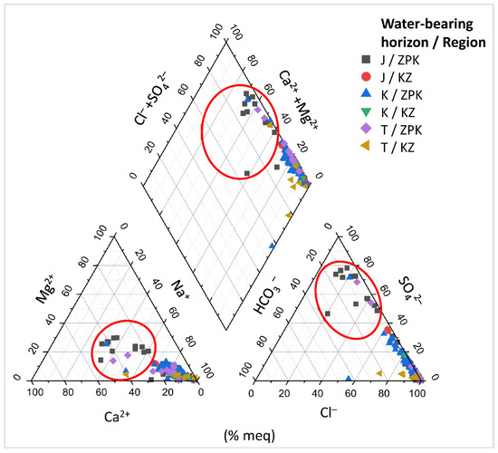
Figure 5.
Piper diagram for the analyzed waters with the division into the water-bearing horizons (K, J, T) and the regions (ZPK, KZ).
2.3. Research Problems
The statistical analyses were aimed at discovering certain dependencies and anomalies related to the water chemistry of the Cretaceous, Jurassic, and Triassic aquifers in the basement of the middle part of the Carpathian Foredeep and in the basement of the middle part of the Outer Carpathians.
We conducted several statistical tests and analyses (details in Section 3.2) to test the hypotheses, to answer the following four questions connected with the chemical composition of the water in the analyzed area:
- In the potentially geothermal waters’ are TDS, the concentrations of the main ions (HCO3−, SO42−, Cl−, Ca2+, Mg2+, Na+, H2SiO3), the values of hydrochemical indices (rNa+/rCl−, rSO42− × 100/rCl−, rHCO3−/rCl−), and the estimated temperature (Tz) significantly different depending on the aquifer (Cretaceous, K, Jurassic, J, and Triassic, T) or region (the Carpathian Foredeep, ZPK, and the Outer Carpathians, KZ)?
- Does the chemical type of the water depend on the depth and mineralization of the water?
- What part of the common variance of the density, TDS, concentration of the main ions (HCO3−, SO42−, Cl−, Ca2+, Mg2+, Na+), values of the indices of metamorphism (rNa+/rCl−), sulphate content (rSO42− × 100/rCl−), and bicarbonate-chlorine (rHCO3−/rCl−), and the estimated temperature (Tz) can be explained by up to three new variables (principal components) as a combination of the analyzed parameters (variables)?
- Can anomalies related to the chemical composition of potentially geothermal waters be found in this new system of variables?
2.4. Applied Research Methods
All statistical tests and the Principal Component Analysis were performed by the author using R (free license open-source statistical software).
The statistical tests used to obtain statistically significant answers to the research questions (1 and 2) included the Kruskal–Wallis test (non-parametric ANOVA), post hoc Duncan test (multiple comparisons of mean values), and Pearson’s Chi-squared (χ2) test. As an auxiliary test for homogeneity of variance, Levene’s test was used. As a test for the normality of distributions, the Shapiro–Wilk test and Anderson-Darling test were used. The purpose of these tests was to check the assumptions for the multivariate version of the ANOVA. The condition of homogeneity of variance in the groups (water-bearing horizon and region) for most parameters (concentration of most ions, density, TDS, H2SiO3, Tz), the condition of data randomization, and the condition of multivariate normality of the distribution were not met (Section 3.1). Therefore, the Kruskal–Wallis test was used, which is a rank test comparing distributions in k > 2 groups, and is most often used when the assumptions for an ANOVA are not met [51]. Then, Duncan’s post hoc tests were performed, which indicated in which groups there were statistically significant differences at the level of 5% significance between the mean values of the analyzed parameters [51]. It is a non-parametric alternative to the Student’s t-test. Pearson’s Chi-squared (χ2) test was performed to check whether the chemical type of the water in the analyzed data was independent of depth (Z) and mineralization (TDS). The formulation of the independence of the tested parameters as the null hypothesis allowed us to state the lack of independence of the tested parameters after rejecting this null hypothesis.
Boxplots (not attached in the article) were used to evaluate the direction of differences between the mean values of the parameters (variables), divided into water-bearing horizons and region.
The methodology of Principal Component Analysis has been described by Jolliffe, I. T. (2002) [52] and Miller and Miller (2005) [53].
Figure 6 shows a flow chart showing what statistical methods were used to try to answer the 4 research questions and where in the article to find the results (Section 2.3).
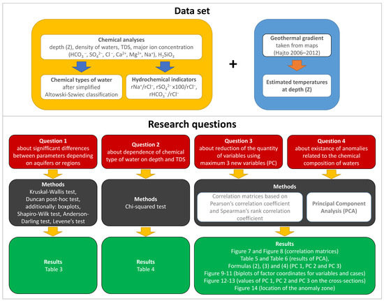
Figure 6.
Flow chart presenting the data set, the scienific problems, used statistical methods and where to find the results.
3. Results
3.1. Statistical Tests
Homogeneity of variance, with respect to the water-bearing horizon (K, J, T) and region (ZPK, KZ), was tested by the Levene’s test to check one of the assumptions for the analysis of variance (ANOVA). The null hypothesis of this test is the homogeneity of variance in a given population. Therefore, the homogeneity of the variance of the parameters (variables) was examined, including the density, TDS, HCO3−, SO42−, Cl−, Ca2+, Mg2+, Na+, rNa+/rCl−, rSO42− × 100/rCl− and rHCO3−/rCl−, as well as Tz, in the groups in relation to the water-bearing horizon (K, J, T) and region (ZPK, KZ).
Only in the case of SO42−, Mg2+ and H2SiO3 did the test not reject the hypothesis of homogeneity of variance. In the remaining cases (density, TDS, HCO3−, Cl−, Ca2+, Na+, Tz) it can be concluded that, at the significance level of 5% (or less), the variance was heterogeneous.
In the groups by region (ZPK, KZ), the null hypothesis of the test of homogeneity of variance was not rejected for the following parameters (variables): density, TDS, HCO3−, Cl−, Ca2+, Mg2+, and Na+. In the remaining cases (SO42−, H2SiO3, rNa+/rCl−, rSO42− × 100/rCl−, rHCO3−/rCl−, Tz) it was found that, at the significance level of 5% (or less), the variance was heterogeneous.
The study of normality of distributions in groups divided by the water-bearing horizon (K, J, T) with the Anderson–Darling and Shapiro–Wilk tests showed that only the parameters (variables) of density, TDS, Cl-, and Na+ for samples from the water-bearing horizon of the Triassic (T) aquifer did not reject the null hypothesis of the normality of distributions. For the remaining tested parameters (variables) from the Cretaceous (K) and Jurassic (J) and for Triassic (T) aquifers—HCO3−, SO42−, Ca2+, Mg2+, H2SiO3, rNa+/rCl−, rSO42− × 100/rCl−, rHCO3−/rCl−, and Tz—the tests rejected the normality of the distribution at a significance level of 5%.
When divided into groups by region (ZPK, KZ), the normality of distributions of all parameters was rejected by tests at the significance level of 5% (or less).
The Kruskal–Wallis test showed that there were no statistically significant (at the significance level of 5%) differences between distributions divided into groups with respect to the water-bearing horizon (K, J, T) for HCO3−, rNa+/rCl−, and rHCO3−/rCl−. The results for H2SiO3 were at the borderline of significance (5%). Thus, it can be said that at the significance level of 10% there were no statistically significant differences between the distributions of H2SiO3 in the Cretaceous (K), Jurassic (J), and Triassic (T) aquifers.
The Duncan test (Holm method, Bonferroni method), performed post hoc, showed which water-bearing horizons (K, J, T) differed significantly in terms of mean values. The interpretation of the results of Kruskal–Wallis test, Duncan’s test and boxplots is presented in Table 3.
Table 3.
Conclusions taken from the Kruskal–Wallis test, Duncan test, and boxplots of statistically significant differences between distributions and mean values, grouped by the water-bearing horizon (K, J and T) and by region (ZPK, KZ).
On the other hand, grouped by region (ZPK, KZ), the Kruskal–Wallis test showed that there were no statistically significant (at the significance level of 5%) differences between the distributions of Mg2+, H2SiO3, and rNa+/rCl− or rHCO3−/rCl−. The rest of the parameters showed statistically significant differences when grouped by region (ZPK, KZ).
The Pearson’s Chi-squared (χ2) test was performed to test or confirm the hypothesis regarding the dependence of the chemical type of the water on the depth of the water sample and on the mineralization of the water. The categorical variable “chemical type” and continuous variables “depth” (Z) and “TDS” were used to perform the test, through converting them into categorical variables by dividing their values into intervals. The ‘depth’ (Z) variable was split every 250 m, and the TDS was split every 10 g/L. The test result for the relationship between the chemical type of the water and the depth (Z) indicated “no independence” between these parameters. Similar conclusions can be drawn in the case of the test result for the study of the independence of the chemical type of the water and mineralization (TDS) (Table 4). Thus, at the significance level of 5%, it can be concluded that the chemical type of the water “is not independent of depth and mineralization”.
Table 4.
Results and interpretation of the Pearson’s Chi-squared test regarding the dependence of the chemical type of water on the depth and TDS.
3.2. Principal Component Analysis
In preparation for the PCA, two versions of the correlation matrix were checked: one based on Pearson’s correlation coefficient (Figure 7), and one based on Spearman’s rank correlation coefficient (Figure 8). The following results were obtained:
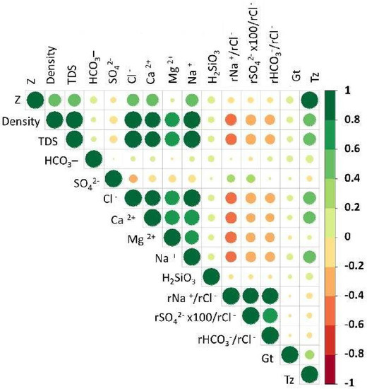
Figure 7.
The correlation matrix based on Pearson’s correlation coefficient.
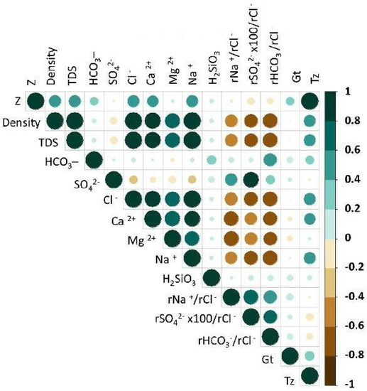
Figure 8.
The correlation matrix based on Spearman’s rank correlation coefficient.
- A negative correlation (50–83%) between the parameters (variables) of rNa+/rCl−, rSO42− × 100/rCl−, rHCO3−/rCl−, Density, TDS, Cl−, Na+, Ca2+, and Mg2+ based on Spearman’s rank correlation coefficient (Figure 8);
- A very low correlation of H2SiO3 with all parameters (variables).
After checking both correlation matrices, it was decided to carry out further analysis of the following parameters (variables): density; TDS; concentrations of the main ions HCO3−, SO42−, Cl−, Ca2+, Mg2+, and Na+; values of the hydrochemical indices rNa+/rCl−, rSO42− × 100/rCl− and rHCO3−/rCl−; and the estimated temperature (Tz).
The variables have different units and are of different orders; therefore, standardization of the variables was used in the analysis. Thus, the PCA was based on the correlation matrix, not the covariance.
The results of Principal Component Analysis (Table 5) indicate how many new variables (PC) should be taken into account, and what percentage of common variance they can explain. For the selection of the number of main components, the Kaiser criterion (components with eigenvalues above 1 are selected), the Cattell’s scree plot (the graph shows a clear gap between the steep inclination of important factors and the gradually decreasing slope of others), and the criterion of a satisfactory percentage were taken into account. A common value was also utilized (in environmental sciences, 60% is required) [51,54].
Table 5.
Importance of components determined by Principal Component Analysis.
For the three principal components (PC 1, PC 2, and PC 3), the eigenvalues exceeded 1 (see the eigenvalues in Table 5). For PC 4, the eigenvalue was close to 1 (0.99); therefore, it was justified to include it in the most important components representing new variables. The percentage of common variance translated by the successive components indicated that PC 1 explains 53%, PC 2–17%, PC 3–9%, PC 4–8%, and PC 5–7% of the variance. This gives a total of 79% of the explained common variance with three principal components, 87% with four principal components, and 94% with five principal components.
Factor loadings indicated which parameters (variables) from among those analyzed had the greatest impact on a given principal component. The factor loadings for the 12 main components are presented in Table 6.
Table 6.
Factor loadings for individual principal components (PC; from 1 to 12).
Since the PCA carried out in this paper was based on the correlation matrix (which was set by the standardization of the variables), the factor loadings could also be treated as correlation coefficients of individual variables with the respective components.
PC 1 was positively correlated with several parameters (variables): density, TDS, Cl−, Ca2+, Na+, Mg2+, and Tz (c.a. above 30% each), and negatively with hydrochemical indices (c.a. −22% each). PC 2 was mainly negatively affected by hydrochemical indices (ca. −50% each). PC 3 was strongly negatively affected by HCO3− (−77%), as well as Tz (−44%), and positively by Mg2+ (c.a. 40%). PC 4 could be identified with one parameter (variable), SO42−, 96%. With four principal components, the percentage of the explained common variance was 87%, and was greater than 79% for three principal components. However, it was decided to adopt the first three components (PC 1, PC 2, PC 3) for further consideration. The interpretation of the new variables was as follows:
- PC 1 is the “weight of water”, and high values are associated with waters of high mineralization and density, and thus increased concentrations of Cl−, Na+, Ca2+, and Mg2+ and elevated temperatures (Tz);
- PC 2 is the “anionic-cationic ratio”, and high values are associated with the lowest values of the selected hydrochemical indices and low temperatures (Tz);
- PC 3 is “magnesium non-bicarbonate”, and high values characterize waters with a low concentration of bicarbonate ions (HCO3-) at an increased concentration of Mg2+ and low temperatures (Tz).
Taking into account all of the analyzed parameters (variables), the equations of these first three principal components can be written as follows:
PC 1 = 0.38∗Density + 0.38∗TDS + 0.38∗Cl− + 0.37∗Na+ + 0.33∗Ca2+ + 0.30∗Mg2+ − 0.26∗rNa+/rCl− −
0.22∗rSO42− × 100/rCl− − 0.21∗HCO3−/rCl− + 0.21∗Tz − 0.11∗SO42− + 0.04∗HCO3
0.22∗rSO42− × 100/rCl− − 0.21∗HCO3−/rCl− + 0.21∗Tz − 0.11∗SO42− + 0.04∗HCO3
PC 2 = − 0.53∗HCO3−/rCl− − 0.51∗rNa+/rCl− − 0.49∗rSO42− × 100/rCl− − 0.25∗Tz − 0.17∗Na+ − 0.16∗TDS −
0.16∗Cl− − 0.16∗Ca2+ − 0.15∗Density − 0.14∗HCO3 − 0.05∗SO42− − 0.01∗Mg2+
0.16∗Cl− − 0.16∗Ca2+ − 0.15∗Density − 0.14∗HCO3 − 0.05∗SO42− − 0.01∗Mg2+
PC 3 = − 0.77∗HCO3 − 0.44∗Tz + 0.40∗Mg2+ + 0.19∗rSO42− × 100/rCl− + 0.09∗HCO3−/rCl− + 0.07∗rNa+/rCl− +
0.06∗Ca2+ + 0.05∗Density + 0.05∗Cl− + 0.04∗TDS − 0.02∗SO42− + 0.02∗Na+
0.06∗Ca2+ + 0.05∗Density + 0.05∗Cl− + 0.04∗TDS − 0.02∗SO42− + 0.02∗Na+
These components are orthogonal to each other, i.e., they are mutually uncorrelated, so they can be used for further analysis (e.g., discriminant or multiple regression) [51].
The projection of the individual factor coordinates of the cases and the factor coordinates of the parameters (variables) on the plane formed by two of the principal components is called a biplot. The axes in the biplot are scaled to show both parameters (variables) and cases (specific water samples) on a single plot. The length of the vectors representing particular parameters (variables) is proportional to the degree of correlation of a given parameter (variable) with particular principal components [51].
The biplots shown are made up of PC 1 and PC 2 (Figure 9), PC 1 and PC 3 (Figure 10), and PC 2 and PC 3 (Figure 11).
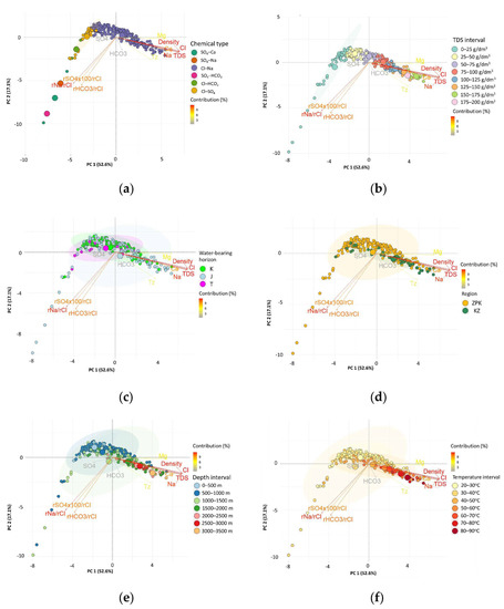
Figure 9.
Biplot of factor coordinates for the cases and variables as a result of the Principal Component Analysis on the surface of PC 1 and PC 2, on the background of: (a) the chemical type of the water; (b) TDS of the water; (c) water-bearing horizon; (d) region; (e) depth; and (f) estimated temperature (Tz).
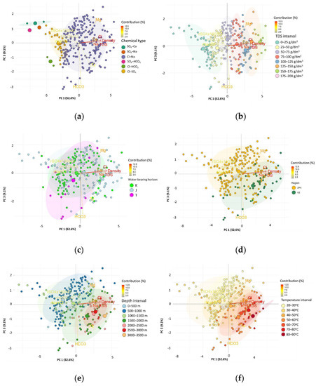
Figure 10.
Biplot of factor coordinates for the cases and variables as a result of the Principal Component Analysis on the surface of PC 1 and PC 3, on the background of: (a) the chemical type of the water; (b) TDS of the water; (c) water-bearing horizon; (d) region; (e) depth; and (f) estimated temperature (Tz).
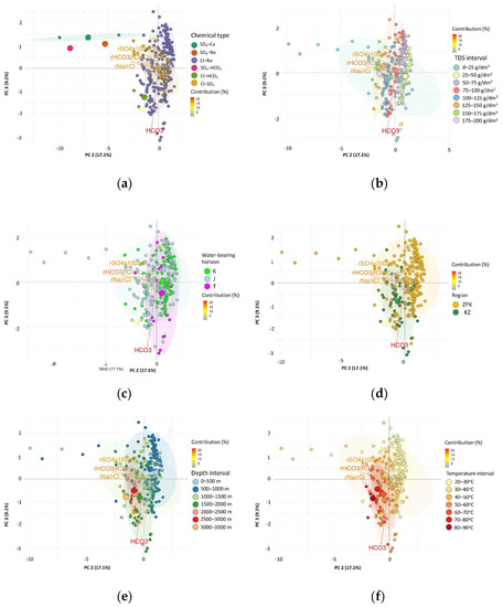
Figure 11.
Biplot of the factor coordinates for cases and variables as a result of the Principal Component Analysis on the surface of PC 2 and PC 3 on the background of (a) the chemical type of the water; (b) TDS of the water; (c) water-bearing horizon; (d) region; (e) depth; and (f) estimated temperature (Tz).
Additionally, the cases (specific water samples) are marked with different colors according to their division into:
The divisions due to TDS intervals, depth intervals, and estimated temperature intervals were used on the biplots as the background for the Principal Component Analysis results. The projection of the cases (water samples) on the PC 1 and PC 2 plane (Figure 9a–f) shows a fairly clear division between the cases belonging to the water of chemical type Cl-Na and the rest of the water types (Figure 9a). Thus, it was possible to determine the value of the factor coordinates for PC 1 (c.a. −2.5), above which the waters only have the Cl-Na type. If the factor coordinates for PC 1 were lower, we were dealing with waters of chemical types SO4-Ca, SO4-Na, SO4-HCO3, Cl-SO4, and Cl-HCO3. On the subsequent biplots it can be read that these chemical types are associated with waters whose TDS does not exceed 25 g/L (Figure 9b). Mostly, these are waters of Jurassic, Cretaceous, and Triassic (K, J, T) (Figure 9c) basement of the Carpathian Foredeep (Figure 9d, factor coordinates for PC 1 < 0 and PC 2 < 0) from a depth range up to a maximum of 1500 m.g.l (Figure 9e), with estimated temperatures (Tz) below 50 °C (Figure 9f). There were no clear differences between waters from the basement of the Carpathian Foredeep (ZPK) and the basement of the Outer Carpathians (KZ), or between waters from the Cretaceous (K), Jurassic (J), and Triassic (T) formations visible on the planes of PC 1 and PC 2.
The projection of cases (water samples) on the PC 1 and PC 3 plane (Figure 10a–f) for the division by chemical type also showed a very clear boundary between the Cl-Na type and other chemical types of water (factor coordinates for PC 1 approx. −2.5). The most negative values of the factor coordinates for PC 1 were related to the chemical types where SO42− was the dominant or one of the dominant anions. Another limit in this division was the value of the PC 3 factor coordinates, which divided the Cl-HCO3 (factor coordinates for PC 3 < 0) from SO4-Ca, SO4-HCO3 and SO4-Cl cases (factor coordinates for PC 3 > 0) (Figure 10a). When divided by TDS intervals, it can be seen that PC 1 is a good discriminator for water types, while PC 3 does not show such properties (Figure 10b). On the other hand, for the values of the factor coordinates for PC 1 < 2 and PC > 0, it can be concluded that the waters came only from the basement of the Carpathian Foredeep (ZPK). Apart from by these values of the factor coordinates PC 1 and PC 3, it was not possible to separate the waters by region of origin. PC 1 and PC 3 also did not distinguish between the Cretaceous (K), Jurassic (J), and Triassic (T) aquifers (Figure 10d). PC 1 and PC 3 did not divide well waters from different depth intervals (Z) (Figure 10e). Similar observations can be made for the partitioning according to the estimated temperature (Tz). However, for the values of the factor coordinates for PC 1 > 1.5 and PC 3 < 0, temperatures above 60 °C can be expected (Figure 10f).
The projection of cases on the PC 2 and PC 3 plane (Figure 11 a–f) indicated that the cases with the lowest values of the factor coordinates for PC 2 were related to the waters of the Jurassic aquifer (Figure 11c) and the basement of the Carpathian Foredeep (Figure 11d). The TDS of these waters did not exceed 25 g/L (Figure 11b), and the depth from which they originated did not exceed 1500 m b.g.l. (Figure 11e), which at the same time affected the value of the estimated temperatures (Tz), which reached a maximum of 40 °C (Figure 11f). With the values of the factor coordinates PC 2 < −2.5 or PC 2 > 0, and at the same time PC 3 > 0, no waters were observed from the basement of the Outer Carpathians (Figure 11d). Most of the waters from the basement of the Outer Carpathians had the value of the factor coordinates PC 3 < 0. These were the waters of the greatest depths (Z) (Figure 11e), and thus with the highest estimated temperatures (Tz), in the range above 50 °C (Figure 11f).
The information from the biplot diagrams (Figure 9, Figure 10 and Figure 11) is complemented by the visualization of the calculated values of the main components of PC 1, PC 2, and PC 3 for the cases (according to Formulas (2)–(4)) in the W–E cross-sections (Figure 12a–c) and the N–S cross-sections (Figure 13a–c). It should be noted that the axis values on the biplots represent the factor coordinates for the individual principal components, as opposed to the calculated values of the individual PC 1, PC 2, and PC 3 components for the cases presented in the cross-sections.
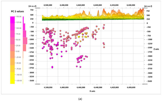
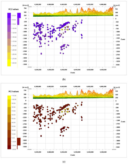
Figure 12.
Cross-section in the line W–E, and values of the principal components (PC), calculated for the cases and viewed from the N. principal components: (a) PC 1; (b) PC 2; (c) PC 3.
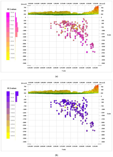
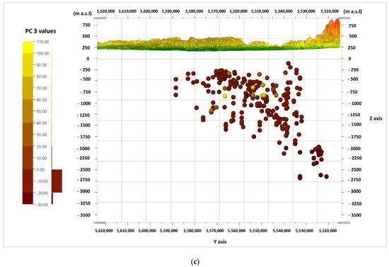
Figure 13.
Cross-section in the line N–S and values of the principal components (PC) calculated for the cases, viewed from the W. principal components: (a) PC 1; (b) PC 2; (c) PC 3.
When looking for potential zones of active water exchange, one should look for zones with lower PC 2 values. Main component PC 1 will also present the lowest values, while PC 3 will present the highest. Therefore, the lowest (negative) values of PC 1 (Figure 12a and Figure 13a) and PC 2 (Figure 12b and Figure 13b), as well as the highest (positive) values of PC 3 (Figure 12c and Figure 13c), are marked with shades of yellow on the cross-sections. They emphasize the existence of the zone, the depth of which can be defined as –500 to –1250 m a.s.l. in the W–E section (Figure 12a–c), and similarly in the N–S section (Figure 13a–c). This zone has different hydrochemical conditions compared to the surroundings. The location of this zone on the map of the analyzed area is shown in Figure 14, where only interesting cases with the lowest values of the main components of PC 1 and PC 2, and the highest values of the PC 3 component, are marked. The zone is located within the Carpathian Foredeep in its central part, in which underground waters are in Jurassic (J) formations under the cover of Cretaceous (K) and Miocene formations of the Carpathian Foredeep. Chemical composition of waters from the zone is presented on the Piper diagram (Figure 5) where one could find samples marked with the red ellipses.
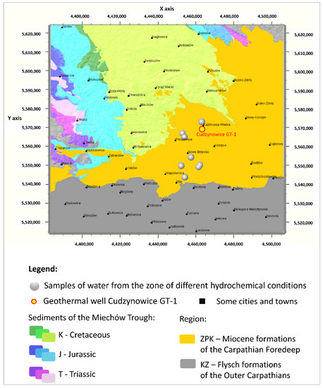
Figure 14.
Location of the zones of different hydrochemical conditions on the background of the geological map of the analyzed area.
4. Discussion
The geological structure of the area in question naturally influences the significant differences in the chemical compositions of the waters. As can be seen in the cross-sections (for example in Figure 3 and Figure 4), the Mesozoic formations of the Miechów Trough plunge under the Miocene formations of the Carpathian Foredeep and the Flysch formations of Outer Carpathians. Thus, the differences in depth generate differences in the mean values of the estimated temperatures (Tz), leading to differences in the mean TDS and all the associated concentrations of the main ions. However, Mg2+ and the hydrochemical indices (rNa+/rCl− and rHCO3−/rCl−) do not show significant differences in mean values due to the origin of the waters from the basement of the Carpathian Foredeep (ZPK) and the basement of the Outer Carpathians (KZ) (Table 3). On the other hand, importantly, the sulfate index, rSO42− × 100/rCl−, differs significantly in waters from the basement of the Carpathian Foredeep and the basement of the Outer Carpathians (Table 3).
The same index shows significant differences in mean values of waters from the Cretaceous (K) and Jurassic (J) formations, while the other hydrochemical indices do not show such differences (Table 3). In the anomaly zone, the hydrochemical indices (rSO42− × 100/rCl−, rNa+/rCl− and rHCO3−/rCl−) negatively affect the value of PC 2 (anion–cationic ratios), which may prove the existence of an active water exchange zone or contact of the water with an active exchange zone. Additionally, low values of PC 1 (water weight) and the lowest PC 3 value (magnesium non-bicarbonate) indicate anomalies and the region with features of waters from active exchange zones. However, it is necessary to consider other possible factors influencing the high values of these indices, reduced mineralization of the waters, and high concentrations of HCO3− ions.
The high rSO42-x100/rCl− value is influenced by increased concentrations of SO42− ions. In the region of the Carpathian Foredeep and its basement (ZPK), the sulfate concentration in the waters of the region in question is influenced by sulfate minerals present in the rocks; the sulfates of the Miocene evaporative level of the Carpathian Foredeep, as well as gypsum and anhydrite in the Mesozoic formations, and the transformation of bitumens (oxidation of the deposits and organic substances scattered in the rock). These processes coexist, and constitute a rich source of sulfur entering the groundwater [55,56]. Its form strongly depends on the redox conditions [16].
Moreover, Nieć (1986) [57] notes that in the Polish deposits of native sulfur (the Carpathian Foredeep), it is possible to observe the movement of sulfur to the bottom of sulfur-bearing formations, within the base of the Baranów sandstones. This is the next step in the conversion of sulfur deposits formed due to the influence of bitumens on gypsum, which is reduced into sulfur-bearing limestone with the participation of bacteria. The excess of bitumens leads to further transformations and, as a result, to leaching of sulfur from sulfur-bearing limestone. Sulfur, in turn, is very easily oxidized to SO42− [16,55,56,57].
The increased content of sulfate ions in the discussed waters may be related to the widespread sulfates in the Miocene evaporative level of the Carpathian Foredeep (ZPK) [21,22,58,59]. Such a relationship was also suggested by Gąsiewicz et al. (2010) [22]. High sulfate index values can result from supply by karst groundwater containing dissolved gypsum [60]. On the other hand, Lipiec et al. (2020) [54] stated that “the proportional relationship between rHCO3 −/rCl− and rSO42− × 100/rCl− ratios (..) suggests inflow from an active water exchange zone”. This thesis was confirmed by the high values of the rNa+/rCl− index, above the average value for ocean water of 0.87 [16,61].
The increased value of the rHCO3−/rCl− index, combined with the decreased mineralization of the waters, may also have a different explanation than the commonly known association of waters of shallower aquifers and active water exchange zones. We were inclined to look for a connection with the processes of destruction of oil deposits, which has also been suggested by other authors [21,38,62]. Waters with low mineralization and a high content of HCO3− ions in areas and reservoirs away from probable supply areas, often adjacent to bitumen deposits, next to Cl-Na, Cl-Ca, and Cl-Mg brines, and sometimes below waters with higher mineralization, as well as bicarbonate waters, are sometimes very slightly mineralized. Some water demineralization is believed to take place there [38]. One of its causes have may been indicated by Lenk (1983) [62]; the dilution of water with water vapor escaping from natural gas deposits during their destruction due to methane (CH4). On the other hand, Gąsiewicz (2000) [21] gave an example of the process taking place during the oxidation of CH4, which, combined with the activity of bacteria, leads to the oxidation of CH4, reduction in SO42−, and production of HCO3− and water (chemically pure). This could provide a good explanation for the influence of hydrocarbon deposits on water chemistry, especially (in this case) enrichment with HCO3− ions and water demineralization.
On the other hand, high values of the rNa+/rCl− index suggest conditions of active water exchange, but high values of TDS could indicate the leaching of sodium-chloride salts, rather than the conditions of good exchange. Therefore, it is important to take into account not only the values of the indices themselves, but also to link them with others that affect the overall picture of the water chemistry.
However, in the area of the described zone with different hydrogeochemical characteristics (Figure 9, Figure 10, Figure 11, Figure 12, Figure 13 and Figure 14), drilling has been undertaken to search for geothermal waters (Cudzynowice GT-1), at the location indicated in Figure 14. The drilling show the existence of zones and water-bearing horizons with good reservoir properties of the rocks of Cretaceous (K) formations. The Cudzynowice GT-1 borehole, which is 750 m deep, was bored with Cenomanian (of the Cretaceous) sands and sandstones, and collects water of a temperature of 27–28.6 °C, mineralization of about 14–15 g/L, and dominant Cl− and SO42− anions. The self-outflow efficiency amounts to 82 m3/h [25].
Hence, taking into account a number of parameters (variables) and combining them into new variables, the principal components may shed new light on the interpretation of the chemical composition of these waters.
5. Conclusions
This paper presents chemical composition of the potentially geothermal waters from statistical point of view and pointing out the hydrochemicaly anomaly zone.
The main achievements of the paper are:
- showing the chemical composition of the waters (based on 268 samples) of the analyzed area (Figure 1, Figure 2, Figure 3 and Figure 4) and indicating statistically significant differences between the waters from the Cretaceous, Jurassic and Triassic aquifers and from the basement of the Carpathian Foredeep (ZPK) and from the basement of the Outer Carpathians (KZ) (Figure 5, Table 1 and Table 2). Statistically significant differences were found between the concentrations of most of the main ions, the TDS, and the density of water in the groups mentioned. On the other hand, HCO3− ions showed no significant differences based on the water-bearing horizon such as Mg2+ ions in the regions (ZPK and KZ). SO42+ ions showed significantly higher mean values in the Carpathian Foredeep than in the basement of the Outer Carpathians (Figure 5, Table 3);
- demonstration that the chemical type of water is “not independent” of mineralization (TDS) and depth (Table 4)—what to expect;
- PCA made it possible to indicate the anomalous zone in comparison of the background in terms of the chemical composition of the waters;
- data preparation (orthogonal new variables—PC) for further analysis—e.g., some of the Discriminant Analyses (LDA, QDA, MDA), Cluster Analysis which would be aimed at finding a good discriminant for water classification based on new statistical methods.
In summary, the chemical composition of the potentially geothermal waters of the basement of the central part of the Carpathian Foredeep and the basement of the Outer Carpathians may have an initial diagnostic role, indicating some anomalies in relation to their background. These may be a symptom of the existence of zones that would be interesting from the point of view of water exploitation for various purposes.
It is worth noting the zone located in the central part of the Carpathian Foredeep in the depth range of –500 to –1250 m a.s.l. mainly related to formations of the Jurassic, but partly also Cretaceous. This zone is different from a hydrogeochemical point of view in relation to the neighboring zones. However, further research is required to attempt to link the chemical composition with various factors influencing its image. It should be considered that the statistical methods and methods of distinguishing an anomalous zone (perhaps indicating conditions for good water exchange) discussed in this article are only auxiliary methods. The used methods have also weak sides for example dependence on estimated temperatures as a substitute for actual temperatures, taking into account hydrochemical indices which are related to main ion concentrations. The methods require supplementing with other methods, especially considering a number of dependencies on the rock mass, hydrogeological and tectonic conditions, and the vicinity of deposits (e.g., hydrocarbons, sulfur, sulfates).
Funding
This research was funded under the AGH-UST statutory research grant No. 16.16.140.315/05.
Institutional Review Board Statement
Not applicable.
Informed Consent Statement
Not applicable.
Data Availability Statement
The data presented in this study are available on request from the corresponding author.
Conflicts of Interest
The author declares no conflict of interest.
References
- Podgorski, J.E.; Labhasetwar, P.; Saha, D.; Berg, M. Prediction Modeling and Mapping of Groundwater Fluoride Contamination throughout India. Environ. Sci. Technol. 2018, 52, 9889–9898. [Google Scholar] [CrossRef] [PubMed]
- Matray, J.M.; Fontes, J.C. Origin of the oil-field brines in the Paris basin. Geology 1990, 18, 501–504. [Google Scholar] [CrossRef]
- Papic, P. Scalling and corrosion potential of selected geothermal waters in Serbia; UNU Geothermal Training Programme, Orkustofnun—National Energy Authority: Reykjavik, Iceland, 1991. [Google Scholar]
- Tomaszewska, B. The prognosis of scaling phenomena in geothermal system using the geochemical modeling methods. Miner. Resour. Manag. 2008, 24, 399–407. [Google Scholar]
- Dzieniewicz, M. Possibilities of using geothermal waters as a raw material for the production of iodine, bromine and other elements. In Proceedings of the Conference: Possibilities of Using Geothermal Waters in Poland with Special Consideration of the Mogilno-Łódź Synclinorium, Ślesin, Poland, 26–27 October 1990; Wyd. AGH: Kraków, Poland, 1990. (In Polish). [Google Scholar]
- Latour, T.; Drobnik, M. Biochemical properties of geothermal waters identified in Poland, determining the manner of their use for therapeutic or recreational purposes. In Geological Exploration Technology, Geothermal Energy, Sustainable Development; No 1; Wyd. IGSMiE PAN: Kraków, Poland, 2016. (In Polish) [Google Scholar]
- Kępińska, B.; Ciągło, J. Possibilities of use of the Podhale geothermal waters for balneotherapeutical and recreational purposes. Geologia 2008, 34, 541–559. (In Polish) [Google Scholar]
- Halaj, E. Geothermal bathing and recreation centres in Poland. Environ. Earth. Sci. 2015, 74, 7497–7509. [Google Scholar] [CrossRef][Green Version]
- Ponikowska, I. Spa Treatment—A Guide for Patients; Oficyna Wydawnicza Branta: Bydgoszcz, Poland, 1996. [Google Scholar]
- Zuber, A.; Ciężkowski, W. Genetic and chemical types of groundwater. Views of the Krakow center. In Regional Hydrogeology of Poland. T. I. Sweet Waters; Panstwowego Instytutu Geologicznego: Warszawa, Poland, 2007. (In Polish) [Google Scholar]
- Zuber, A.; Chowaniec, J.; Porwisz, B.; Najman, J.; Mochalski, P.; Śliwka, I.; Duliński, M.; Mateńko, T. The origin and age of mineral waters in the Busko-Zdrój region, determined on the basis of environmental markers In Sulfate Waters in the Busko-Zdrój Region; Hydrogeotechnika Sp. o.o.: Kielce, Poland, 2010. (In Polish) [Google Scholar]
- Sekuła, K.; Rusiniak, P.; Wątor, K.; Kmiecik, E. Hydrogeochemistry and Related Processes Controlling the Formation of the Chemical Composition of Thermal Water in Podhale Trough, Poland. Energies 2020, 13, 5584. [Google Scholar] [CrossRef]
- Macioszczyk, A.; Dobrzyński, D. Hydrogeochemistry. Zone of Active Groundwater Exchange; Wydawnictwo Naukowe PWN: Warszawa, Poland, 2002. (In Polish) [Google Scholar]
- Marszałek, H.; Rysiukiewicz, M. Aluminium in waters of the active exchange zone in the Karkonosze National Park (Western Sudetes, SW Poland). Bull. Geogr. Phys. Geogr. Ser. 2019, 17, 101–110. [Google Scholar] [CrossRef]
- Paczyński, B.; Płochniewski, Z. Mineral and Healing Waters of Poland; Państwowy Instytut Geologiczny: Warszawa, Poland, 1996. (In Polish) [Google Scholar]
- Macioszczyk, A. Hydrogeochemistry; Wydawnictwa Geologiczne: Warszawa, Poland, 1987. (In Polish) [Google Scholar]
- Appelo, C.A.J.; Postma, D. Geochemistry, Groundwater and Pollution; Balkema: Rotterdam, The Netherlands, 1999. [Google Scholar]
- Mazor, E. Chemical Isotopic Groundwater Hydrology, 3rd ed.; Marcel Dekker, Inc.: New York, NY, USA; Marcel Dekker, Inc.: Basel, Switzerland, 2004. [Google Scholar]
- Karnkowski, P. Oil and Gas de Posits in Poland; Towarzystwo Geosynoptyków “Geos”: Kraków, Poland, 1999. [Google Scholar]
- Gągulski, T.; Gorczyca, G. Diversification of geothermal conditions of the cenomanian water-bearing system on the example of new drillings from the Busko-Spa region. Geol. Explor. Technol. Geotherm. Energy Sustain. Dev. 2018, 57, 73–84. (In Polish) [Google Scholar]
- Gąsiewicz, A. Sedimentology and diagenesis of gypsum-ghost limestones and origin of Polish native sulphur deposits. Prace Państw. Inst. Geol. 2000, 172, 1–143. (In Polish) [Google Scholar]
- Gąsiewicz, A.; Drzewicki, W.; Jezierski, P. Isotope composition of sulfur in therapeutic sulphide waters in the Busko-Zdrój region—implications for genesis. In Sulfate Waters in the Busko-Zdrój Region; Hydrogeotechnika Sp. o.o.: Kielce, Poland, 2010. (In Polish) [Google Scholar]
- Chowaniec, J.; Gągulski, T.; Gorczyca, G. Occurrence and origin of healing waters in Jurassic formations of the Busko-Zdrój and Solec-Zdrój regions. In 3. Polish Geological Congress. Challenges of Polish Geology; PTG-SGP: Wrocław, Poland, 2016. (In Polish) [Google Scholar]
- Lisik, R.; Szczepański, A. Sulphide Healing Waters in a Part of the Carpathian Foredeep; Hydrogeotechnika Sp. o.o.: Kielce-Kraków, Poland, 2014. (In Polish) [Google Scholar]
- Wiktorowicz, B.; Nowak, J. The geothermal waters in the Kazimierza Wielka region and the possibilities for use. In Geological Exploration Technology, Geothermal Energy, Sustainable Development; No 2; Wyd. IGSMiE PAN: Kraków, Poland, 2016. (In Polish) [Google Scholar]
- Oszczypko, N.; Tomaś, A. Creataceous water-bearing horizons in the middle part of the Carpathian Foredeep. Zesz. Nauk. AGH Geologia 1976, 2, 79–91. (In Polish) [Google Scholar]
- Oszczypko, N.; Tomaś, A. Characteristics of reservoir properties of Jurassic sediments of the Carpathian Foredeep. Kwart. Geol. 1978, T. XX, 3. (In Polish) [Google Scholar]
- Oszczypko, N.; Zuber, A. Geological and isotopic evidence of diagenetic waters in the Polish Flysch Carpathians. Geologica Carpathica 2002, 53, 257–268. [Google Scholar]
- Pich, J. Chemistry of the groundwaters in the middle part of the Carpathian Foredeep. Biul. Inst. Geol. 1978, 4, 73–89. (In Polish) [Google Scholar]
- Chowaniec, J.; Felisiak, I. The genesis of mineralization of the waters of the Mateczny health resort in Kraków. In Tradition and Modernity in Sedimentological Interpretations. IV National Meeting of Sedimentologists; International Association of Sedimentologists: Kraków, Poland, 1995. (In Polish) [Google Scholar]
- Chowaniec, J. Hydrogeology study of the western part of the Polish Carpathians. Hydrogeologia, Z. VIII. Biul. Państw. Inst. Geol. 2009, 434, PIG-PIB. (In Polish) [Google Scholar]
- Chowaniec, J.; Najman, J.; Olszewska, B.; Zuber, A. Origin and age of mineral water at Dobrowoda near the Busko Spa. Przegl. Geol. 2009, 57, 286–293. (In Polish) [Google Scholar]
- Chowaniec, J.; Ciężkowski, W.; Duliński, M.; Józefko, I.; Porwisz, B.; Zuber, A. Chemical facies of CO2-rich waters in the Flysch Carpathians versus water age. Biul. Państw. Inst. Geol. 2009, 436, 47–54. (In Polish) [Google Scholar]
- Chowaniec, J.; Najman, J.; Mochalski, P.; Śliwka, I.; Zuber, A. The origin of mineral waters in Kraków. Biul. Państw. Inst. Geol. 2011, 445, 35–42. (In Polish) [Google Scholar]
- Wątor, K.; Kmiecik, E.; Lipiec, I. The use of principal component analysis for the assessment of the spatial variability of curative waters from the Busko-Zdrój and Solec-Zdrój region (Poland)—preliminary results. Water Supply 2019, 19, 1137–1143. [Google Scholar] [CrossRef]
- Gała, I. Hydrochemical characteristics of sulphide thermal waters in the Busko C-1 borehole. In Geological Exploration Technology, Geothermal Energy, Sustainable Development; No 2; Wyd. IGSMiE PAN: Kraków, Poland, 2013; pp. 117–126. (In Polish) [Google Scholar]
- Gorczyca, G.; Chowaniec, J.; Gągulski, T. Characteristics of geothermal water of the Cenomanian aquifer system at the boundary of the SE part of the Miechów Basin and the Carpathian Foredeep. Przegl. Geol. 2017, 65, 237–246. (In Polish) [Google Scholar]
- Kotlicki, S. Groundwater chemistry of the south-western part of the Miechów Trough. Biul. Inst. Geol. 1971, 1, 249. (In Polish) [Google Scholar]
- Krawczyk, J.; Mateńko, T.; Mądry, J.; Porwisz, B. Healing waters of Busko Zdrój in the light of previous research. In Contemporary Problems of Hydrogeology, T. IX; PIG: Warszawa-Kielce, Poland, 1999. (In Polish) [Google Scholar]
- Lisik, R. Healing sulphide waters of the Pińczów-Busko-Zdrój-Kazimierza Wielka region. In Sulfate Waters in the Busko-Zdrój Region; Hydrogeotechnika Sp. o.o.: Kielce, Poland, 2010. (In Polish) [Google Scholar]
- Motyka, J.; Rajchel, L. Mineral waters and acratopegs. In Model Study of Comprehensive Use and Protection of Balneological Raw Materials in Krakow and the Surrounding Area; Ney, R., Ed.; Wyd. IGSMiE PAN: Kraków, Poland, 2002. (In Polish) [Google Scholar]
- Motyka, J.; Porwisz, B.; Rajchel, L.; Zuber, A. Mineral waters of Krzeszowice. In Contemporary Problems of Hydrogeology; T. IX, Part 1; Politechnika Gdańska: Gdańsk, Poland, 2003; pp. 129–135. (In Polish) [Google Scholar]
- Sowiżdżał, A.; Jasnos, J. Hydrochemical characteristics of the groundwaters. In Geothermal Atlas of the Carpathian Foredeep; Górecki, W., Sowiżdżał, A., Jasnos, J., Papiernik, B., Hajto, M., Machowski, G., Kępińska, B., Czopek, B., Kuźniak, T., Kotyza, J., et al., Eds.; Goldruk: Kraków, Poland, 2012. (In Polish) [Google Scholar]
- Jasnos, J. Characteristics of mineral, specific, healing waters and brines. In Geothermal Atlas of the Carpathian Foredeep; Górecki, W., Sowiżdżał, A., Jasnos, J., Papiernik, B., Hajto, M., Machowski, G., Kępińska, B., Czopek, B., Kuźniak, T., Kotyza, J., et al., Eds.; Goldruk: Kraków, Poland, 2012. (In Polish) [Google Scholar]
- Jasnos, J. Occurrences of mineral waters, waters containing specific components and brines recorded in the petroleum-prospecting wells. In Geothermal Atlas of the Eastern Carpathians; Górecki, W., Hajto, M., Augustyńska, J., Jasnos, J., Kuśmierek, J., Kuźniak, T., Machowski, G., Machowski, W., Nosal, J., Michna, M., et al., Eds.; Goldruk: Kraków, Poland, 2013. [Google Scholar]
- Jasnos, J. Geothermal Conditions of the Mesozoic Formations in the Miechów Trough. Ph.D. Thesis, AGH—University of Science and Technology, Kraków, Poland, 2019. Unpublished. (In Polish). [Google Scholar]
- Hajto, M. Distribution map of terrestrial heat flow density in the Polish Lowlands. In Atlas of Geothermal Resources of Mesozoic Formations in the Polish Lowlands; Górecki, W., Szczepański, A., Sadurski, A., Hajto, M., Papiernik, B., Kuźniak, T., Kozdra, T., Soboń, J., Szewczyk, J., Sokołowski, A., et al., Eds.; Goldruk: Kraków, Poland, 2006. [Google Scholar]
- Hajto, M. Geothermal analysis of the Polish Western Carpathians. In Atlas of Geothermal Waters and Energy Resources in the Western Carpathians; Górecki, W., Szczepański, A., Oszczypko, N., Hajto, M., Oszczypko-Clowes, M., Papiernik, B., Kępińska, B., Czopek, B., Haładus, A., Kania, J., et al., Eds.; Goldruk: Kraków, Poland, 2011. [Google Scholar]
- Hajto, M.; Szewczyk, J. Geothermal analysis of the Carpathian Foredeep area. In Geothermal Atlas of the Carpathian Foredeep; Górecki, W., Sowiżdżał, A., Jasnos, J., Papiernik, B., Hajto, M., Machowski, G., Kępińska, B., Czopek, B., Kuźniak, T., Kotyza, J., et al., Eds.; Goldruk: Kraków, Poland, 2012. (In Polish) [Google Scholar]
- Altowskij, M.E.; Szwiec, W.M. On the question of the nomenclature of the chemical composition of groundwater. Sat. Problems of hydrogeology and engineering geology; No 14; Gos Geoltekhizdat: Moscow, Russia, 1956. [Google Scholar]
- Stanisz, A. An Accessible Statistics Course with the Use of Statistica PL on Examples from Medicine. Volume 3. Multivariate Analyzes; Statsoft: Kraków, Poland, 2007. (In Polish) [Google Scholar]
- Jolliffe, I.T. Principal Component Analysis; Springer: Cham, Switzerland, 2002. [Google Scholar]
- Miller, J.N.; Miller, J.C. Statistics and Chemometrics for Analytical Chemistry, 5th ed.; Pearson Education: Harrow, UK, 2005. [Google Scholar]
- Lipiec, I.; Wątor, K.; Kmiecik, E. The application of selected hydrochemical indicators in the interpretation of hydrogeochemical data—A case study from Busko-Zdrój and Solec-Zdrój (Poland). Ecol. Indic. 2020, 117. [Google Scholar] [CrossRef]
- Różkowski, J.; Jóźwiak, K.; Andrejczuk, V. Chemistry of groundwater in gypsiferous Badenian series in the northern part of the Carpathian Foredeep. Biul. Państw. Inst. Geol. 2011, 445, 573–582. [Google Scholar]
- Turek, S. Analysis of relations between hydrogeological conditions and distribution of sulfur deposits in the Miocene in the Carpathian Foredeep. Przegl. Geol. 1983, 31, 482–485. [Google Scholar]
- Nieć, M. Sulfur deposits transforming processes. Przegl. Geol. 1986, 34, 7. [Google Scholar]
- Szuflicki, M.; Malon, A.; Tymiński, M.; Bońda, R.; Brzeziński, D.; Czapigo-Czapla, M.; Czapowski, G.; Fabiańczyk, J.; Kalinowska, A.; Malon, A.; et al. Balance of Minerals and Groundwater Resources in Poland as of 31.XII. 2019; Tymiński, M., Ed.; PIG-PIB: Warszawa, Poland, 2020. (In Polish) [Google Scholar]
- Barbacki, A.P. Geothermal water reservoirs of the Miechów Trough and the central part of the Carpathian Foredeep. In Studia Rozprawy Monografie; IGSMiE PAN: Kraków, Poland, 2004. (In Polish) [Google Scholar]
- Han, D.; Liang, X.; Jin, M.; Currell, M.J.; Han, Y.; Song, X. Hydrogeochemical indicators of groundwater flow systems in the Yangwu River alluvial fan, Xinzhou Basin, Shanxi, China. Environ. Manage 2009, 44, 243–255. [Google Scholar] [CrossRef] [PubMed]
- Pazdro, Z.; Kozerski, B. General hydrogeology; Wydawnictwa Geologiczne: Warszawa, Poland, 1990. (In Polish) [Google Scholar]
- Lenk, T. (Ed.) Geological Structure, Structural, Facies and Geochemical Conditions as well as Prospects for Exploration of Natural Gas Deposits in the Miocene Deposits in the Vicinity of the Shore and under the Carpathian Thrust; Pr. Inst. Górnict. Naft. i Gazown; No. 45; Inst. Górn. Naft. i Gazown.: Kraków, Poland, 1983. (In Polish) [Google Scholar]
Publisher’s Note: MDPI stays neutral with regard to jurisdictional claims in published maps and institutional affiliations. |
© 2021 by the author. Licensee MDPI, Basel, Switzerland. This article is an open access article distributed under the terms and conditions of the Creative Commons Attribution (CC BY) license (https://creativecommons.org/licenses/by/4.0/).