Abstract
One of the methods of heat transfer enhancement is utilization of the turbulent impinging jets, which were recently applied, for example, in the heat exchangers. Their positive impact on the heat transfer performance was proven, but many questions related to the origin of this impact are still unanswered. In general, the wall-jet interaction and the near-wall turbulence are supposed to be its main reason, but their accurate numerical analysis is still very challenging. The authors’ aim was to construct the numerical model which can represent the real phenomena with good or very good accuracy. Starting with an analysis of single jet and obtaining the agreement with experimental data, it will be possible to extend the model towards the whole minijets heat exchanger. The OpenFOAM software, Bracknell, UK was used for that purpose, with our own implementation of the ζ-f turbulence model. The most difficult area to model is the stagnation region, where the thermal effects are the most intensive and, at the same time, strongly affected by the conditions in the pipe/nozzle/orifice of various size (conventional, mini, micro), from which the jet is injected. In the following article, summary of authors’ findings, regarding significance of the velocity profile and turbulence intensity at the jet place of discharge are presented. In addition, qualitative analysis of the heat transfer enhancement is included, in relation to the inlet conditions. In the stagnation point, Nusselt number differences reached the 10%, while, in general, its discrepancy in relation to inlet conditions was up to 23%.
1. Introduction
Various flows occurring in the engineering systems can be turbulent and their accurate scientific analysis is still very challenging. One of the methods of heat transfer enhancement is utilization of the turbulent impinging jets [1,2]. Jet impingement, phenomena occurring when the fluid stream hits the surface, is an example of a very demanding topic for the researchers, especially when combined with the heat transfer [3]. The available results, obtained by the numerical and experimental approaches, very often share the same unsolved drawback: lack of universality.
To make it more general, it is a common practice to present the obtained data in a non-dimensional way. Such representation can be found in numerous articles and books regarding the topic of the jet impingement. As this phenomenon is used to enhance the heat transfer rates, the typical results presented in such publications consist of the hydrodynamic and thermal data, for example, the local and mean values of Nusselt number on the impinged surface, defined by Equation (1),
for local velocity profiles, local values of normal and shear stresses, turbulence parameters, etc. They are obtained at various values of Reynolds number calculated at the jet inlet, defined by Equation (2),
and some geometrical parameters, such as H/D ratio, representing the distance H between the pipe/nozzle/orifice and the impinged wall, divided by the pipe/nozzle/orifice diameter, D. The meaning of symbols from Equations (1) and (2) are as follows: αef is the so-called effective heat transfer coefficient, W/(m2∙K), which takes into account an impact of the turbulence on the convective heat transfer by using the eddy diffusivity approach [4]; λ is the thermal conductivity of the fluid, W/(m∙K); ub is the bulk velocity at the inlet, m/s; and ν is the kinematic viscosity, m2/s.
Such non-dimensional approach can be seen in numerous publications, just to mention Grenson et al. [5] or Yadav and Agraval [6]. Information about the exact values of the diameter or other geometrical parameters is usually available; however, it is not always comprehensive information, especially for the research based on the numerical approach. Unexperienced readers can easily get the conclusion that some published results from particular sources can be treated as absolute and universal (for a given constraint, for example, Reynolds number or the ratio of H/D)—but, it is not right. The research presented by Lee and Lee [7] and Donovan and Murray [8] has revealed that impinging jet flows at the same Reynolds number but at different values of the inlet pipe diameter lead to discrepancy in the Nusselt number.
The explanation of these differences is related to the research done by Garimella and Nenaydykh [9], who investigated the effect of nozzle geometry (diameter, H/D ratio, nozzle wall thickness) on the local heat transfer coefficients. The analyzed cases referred to a single jet with nozzle diameters in the range of 7 × 10⁻⁴ to 6.35 × 10⁻³ m and also various nozzle aspect ratios in the range of 0.25–12, at constant Reynolds number and H/D ratio. They indicated considerable differences between the results in the stagnation zone for all analyzed cases. The stagnation point results were even two times higher for double inlet diameter. In addition, they have shown the substantial impact of nozzle shape on the obtained results. The conclusions presented in Reference [9] were confirmed by Lee et al. [10], who also obtained different thermal results in the stagnation zone, depending on the inlet dimension. In their opinion, the reason was connected with the intensity of turbulence in the jet core, variable for different inlet diameters. Royne and Dey [11] studied an influence of nozzle shape on the results and indicated similar findings. The problem becomes even more complex when possible effect of the differences in the experimental methods and inaccuracy of error estimation are considered. It was discussed by Zhou et al. [12], who have shown that even small changes of particular elements of the experimental system, such as thickness of the impinged and heated plate, lead to various results of the heat transfer intensity.
The long-term aim of authors’ research is to construct the numerical model assuring the results as close as possible to the experimental ones in the case of single jet and jets array and then model the transport processes in the minijets heat exchanger [1]. At first, however, it is necessary to clarify the uncertainties reported in the literature. Therefore, in this paper, the research regarding an influence of inlet flow definition on the thermal processes occurring during the jet impingement on the flat surface is discussed. It develops the idea of turbulence intensity significance raised by Lee et al. [10]. To evaluate its impact, qualitative analysis of the heat transfer enhancement is included, in relation to two various turbulent inlet conditions. The results, regarding the thermal and hydrodynamic boundary layers, turbulence kinetic energy, and its budget, together with the enstrophy flux analysis, are presented and discussed.
2. Numerical Considerations
Simulations were performed with the use of OpenFOAM (GNU General Public Licence, v2006, ESI-Open CFD, Bracknell, UK), the finite volume based, open-source software. It also allows us to implement user-programmed functionalities, which were used in the case of ζ-f model and other work conducted for the purposes of presented work.
2.1. Numerical Model
The jet impingement numerical analyses require the conservation laws of mass, as in Equation (3); momentum, as in Equation (4); and energy, as in Equation (5), to be combined [4]. In the article, the Reynolds Averaged Navier–Stokes (RANS) approach is considered:
where ui,j are the components of velocity vector, m/s; ρ is the fluid density, kg/m3; p is the pressure, Pa; μ is the fluid dynamic viscosity, Pa·s; Sij is the tensor of strain rate, 1/s;
is the term for the Reynolds stress tensor, m2/s2; Θ is the mean fluid temperature, K;
is the fluctuation of fluid mean temperature, K; a is the thermal diffusivity, m2/s and
represents the turbulent heat fluxes, K∙m/s.
As analyzed flow was turbulent for the assumed conditions, it was necessary to combine the Navier–Stokes equations with the appropriate turbulence modeling. Turbulent heat fluxes were modeled with the use of the turbulent Prandtl number [4]. While other, more advanced formulations were also proposed to be coupled with RANS-based turbulence models, such as the one of Kenjeres, Gunarjo, and Hanjalic [13], that basic approach is also capable of providing sufficient results.
The selected RANS model was the Hanjalic’s et al. ζ-f model [14]. Authors proved it is suitable for the jet impingement simulations [15,16]. This model consists of four additional equations system, representing k (turbulence kinetic energy), ε (the dissipation of k), ζ (fluctuation of the velocity normal to streamlines
normalized by k), and f (relaxation function), which plays a major role in controlling the turbulence production near the wall:
where G is the turbulence kinetic energy production term, m2/s3, Cε1, Cε2, C1, C’2, σk, σε, and σζ are the model specific constants, τ is the time scale, and L is the length scale.
The introduction of two additional (in comparison to conventional k-ε turbulence models) variables, ζ and f, leads to improved accuracy of simulating near-wall momentum and energy transport, as they represent the possible impact of anisotropic turbulent phenomena (even though the model itself still assumes the isotropic turbulence, similarly as majority of other RANS models). The aforementioned ζ-f turbulence model is not typically available in Computational Fluid Dynamics (CFD) software. It could only be used after implementing it into the software, which was successfully done.
The steady-state cases were considered. Therefore, Semi-Implicit Method for Pressure Linked Equations (SIMPLE) algorithm had to be used to control the pressure-velocity coupling. Its basic operations are as follows [4]:
- initialize ui+1 and pi+1,
- construct and under-relax the momentum equation,
- solve the momentum equation to obtain prediction for ui+1,
- solve the momentum equation to obtain the prediction for ui+1,
- construct and solve the pressure equation for pi+1,
- correct the cell surface flux and under-relax pi+1,
- correct the velocity ui+1, and
- check the convergence, move to iteration i + 2, or repeat the algorithm.
All utilized schemes were of second-order accurate, namely linear Upwind for divergence operator and Gauss linear for gradients, with cell-based limiters for velocity and turbulence variables to control the solution progress, especially at the initial iterations [4]. Convergence rate of residuals was set to reach the values below 1 × 10⁻⁸. Nevertheless, the average Nusselt number at the impinged surface was also monitored to identify the occurrence of steady-state conditions.
2.2. Geometry and Boundary Conditions
A working fluid was the air, characterized by the properties listed in Table 1. Due to small temperature difference in the simulated process, these properties were considered as constant. The type and placement of the boundary conditions are presented in Figure 1, together with an important geometrical parameters, such as x – radial variable from the stagnation point, which is used to define the non-dimensional distance along the heated surface x/D, and h—variable representing a distance between the stagnation point and the potential jet core termination, which is used to define the non-dimensional distance, h/D.

Table 1.
Working fluid (the air) properties.
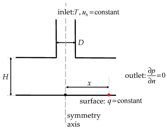
Figure 1.
Boundary conditions placement. Indication of important geometrical variables. Further explanation is included in Table 2.
At the inlet, the developed profile was achieved by using the OpenFOAM specific feature that allows the recycling (mapping) of the upstream flow parameters (after initializing with the predefined conditions) back to the inlet with every iteration, what simulates the existence of the infinitely long initial channel. It also allows to maintain constant bulk velocity at the mapped inlet. Impinged surface was heated with the constant heat flux, q. Its value was taken from the existing analysis of the heat exchanger [1]. The values at boundaries are listed in Table 2.
Table 2.
Boundary conditions.
2.3. Mesh Details
It is important to mention that considered cases were axisymmetric, due to the nature of investigated phenomenon. As a result, it allowed us to reduce the necessary amount of mesh elements. All elements were hexahedral, apart from wedges at the symmetry axis proximity. Up to 66,000 elements were generated. In Figure 2, the results of the mesh independence tests are presented. As the ζ-f model is the low-Reynolds type of RANS model, it requires the mesh to be dense enough to define the near-wall flow properties. In addition, the mesh was refined at the zones of higher gradients of particular variables and along the direction of the flow. As it can be seen, apart from the most basic mesh, two others provided complementary results, and there was no need for further refinement.
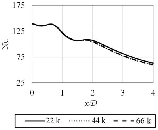
Figure 2.
The mesh independence test results, conducted for selected number of mesh elements. Boundary conditions equal to those listed in Table 2.
The common practice in an analysis of the heat transfer processes is to keep the dimensionless first node distance from wall y+, defined in Equation (11), at values of about 1 to fully simulate the boundary layer [4]. While it is possible to use the ζ-f model in combination with the wall-functions, as proposed by Popovac and Hanjalic [17], such approach was omitted in the presented paper to achieve an effect from the previous sentence.
where y is the distance between the wall and the first mesh node near it, m and u* is the friction velocity, m/s. For the purposes of presented research this criterion was lowered to 0.5 to increase the near-wall mesh refinement.
2.4. Validation of ζ-f Model
In Figure 3, selected validation data of ζ-f model is presented, in the basis of comparison between the experimental data [18] and the numerical results obtained with the utilization of typical k-ε [4] and ζ-f models. It is related to the wall-normal flow conditions and the boundary layer is generated due to jet impingement. As can be seen, the agreement obtained when using the Hanjalic’s model is significantly higher.
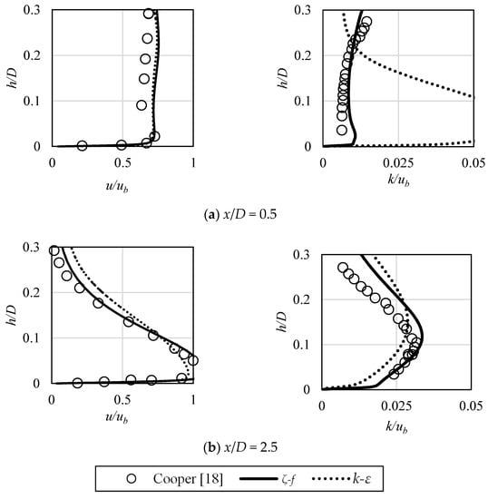
Figure 3.
Numerical model validation. Reference experimental data [18] versus k-ε and ζ-f models results. Velocity profiles (left side) and turbulence kinetic energy profiles (right side) for indicated values of non-dimensional distance x/D from stagnation point.
An agreement of the ζ-f model based results with the validation data was the most important factor, but also the relative time of simulations was an added value and an important aspect for the future, more complex simulations. While this model can be perceived as the improved version of classical k-ε model, its formulation was based on many assumptions originated from various turbulence modeling approaches [14]. It allowed to minimize the drawbacks of the eddy viscosity models, especially the overprediction of the turbulence production in the flow stagnation areas, where the velocity values are relatively small, but the vorticity reaches high values.
3. Preliminary Research
3.1. Issues of Non-Dimensionalization
The issue mentioned in the Introduction, an accurate understanding of non-dimensional data from scientific literature regarding jet impingement is especially challenging when it comes to the numerical works. However, it is not limited only to them. An example of possible significant discrepancies can be shown based on experimental results by Lee and Lee [7] and Donovan and Murray [8]. In their publications, local Nusselt number values at various Reynolds numbers, calculated for the jet inlet and particular H/D cases, were shown. For both inlets, the Reynolds number was equal to 20,000, and the flow leaving the pipe was described as fully developed. The only noticeable difference was the actual diameter of the pipe, in which the inlet conditions were generated; in Reference [7], it was 0.025 m, in Reference [8], 0.0135 m. An example of possible significant discrepancies is presented in Figure 4, which summarized their findings related to the Nusselt number at the impinged surface. In Figure 4a, the case corresponds to the ratio H/D = 2; in Figure 4b, the case is H/D = 4. Inlet Reynolds number was equal to 20,000.
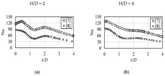
Figure 4.
Experimental results of jet impingement analysis [7,8]. Inlet Reynolds number equal to 20,000, (a) H/D = 2, (b) H/D = 4.
As can be concluded, the differences are noticeable, not only for the results along the surface, at which Nusselt number was calculated, but also within the stagnation zone.
While previously referenced research [7,8,9,10,11] concerned the experimental investigations, the authors, in their own numerical research, also obtained similar discrepancies in the results, as presented in Figure 5, where effect of a relative increase of the diameter size on the thermal performance results is visualized. For both cases, the working fluid, its properties, inlet conditions (Reynolds number equal to 30,000, inlet temperature equal to 300 K, fully developed turbulent conditions), and outlet definition were exactly the same. In addition, numerical configurations did not differ.
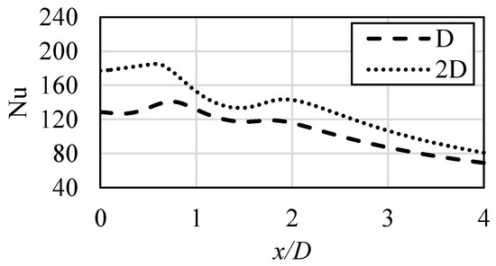
Figure 5.
Comparison of numerical results obtained at constant inlet Reynolds number Re = 30,000, constant H/D = 2 and various values of the inlet diameter. ζ-f turbulence model, authors’ own research.
The majority of the available software packages are based on the finite element, volume, or difference methods. The computational time of particular simulation depends mostly on a number of these discrete parts, which together represent the real model. Therefore, it is important and common practice of CFD users to reduce their number. Typically, the fully developed flow is generated with a usage of mapped/periodic boundary conditions techniques, instead of creating the mesh and simulating long enough pipes for the flow to develop. As it will be proved in the next pages, such an approach can lead to different results. Additionally, typical CFD meshing manipulation techniques might lead to other paradox situations. From the CFD methods point of view, there is no difference between the mesh of one shape and another corresponding mesh, in which all the distances between nodes were obtained by the multiplication of the same distances from the first mesh. As a result, even with complete change of geometry, obtained results would not vary between two meshes; an example might be the simulation of two various pipe flows, of different diameters. In reality, on the other hand, such flows are characterized by different conditions, as indicated, for example, in Figure 4 and Figure 5.
3.2. Inlet Turbulence Definition
To analyze the problem mentioned in the previous section, two various profiles at the inlet were investigated. Varying parameters, defining it, chosen in accordance with the method of Behnia et al. [19,20], are listed in Table 3.
Table 3.
Investigated conditions at the inlet.
The turbulence intensity I was calculated with the utilization of Equation (12) [4]:
where u′ is the velocity fluctuation, m/s; and k is the turbulence kinetic energy, m2/s2.
As it can be concluded, the applied ζ-f model assumes the isotropic fluctuations of the velocity.
In Figure 6, the velocity profiles, as well as the profiles of turbulence intensity, I, are shown, with noticeable differences between investigated cases. The velocity ratio uc/ub represents the centerline velocity uc divided by the bulk velocity ub. For both cases, the second value remained the same, which allowed the comparison. The “case I” can be, though, as the software-related fully developed profile, obtained by the inlet mapping technique. The “case II” represents the values obtained by simulation of already developed flow through the circular pipe. It can be seen, when analyzing Figure 6a, that bigger differences between the values occurred for the turbulence intensity, as shown in Figure 6b. Nevertheless, it also can be noticed that the near-wall values of the turbulence intensity do not differ significantly, which indicates and proves the fact that the boundary layer is already established in both cases.
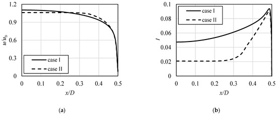
Figure 6.
The velocity profiles (a) and the turbulence intensity I (b) at the inlet, for both analyzed cases.
4. Results of Main Studies and Discussion
The boundary conditions listed in Table 2 were selected as they refer to the widely used benchmark case, presented, and verified by the ERCOFTAC (European Research Community on Flow, Turbulence and Combustion) Association. It is based on the experimental investigation of Yan [21] and Cooper et al. [18], as well as Baughn and Shimizu [22]. Some numerical insight about the case is provided in Reference [19,20].
In Figure 7, the Nusselt number results obtained at the impinged surface with both inlet conditions are presented, in reference to verified experimental data [21]. Close to the stagnation point, different results can be observed, while, away from the stagnation point, where the wall jet is already generated and developed, minor differences can be seen, and the tendency is constant (“case I” providing slightly higher values of convective heat transfer). At the stagnation point, the values obtained with “case I” assured better accuracy. However, the important feature of local Nusselt number curve, its secondary peak, that occurs for particular combinations of H/D and Reynolds numbers [15,16], was significantly better expressed when the “case II” was used. Its physical meaning is related to the fact that, while first peak originates from the jet features itself intensifying the heat transfer, the latter is generated during the formation and evolution of impinging surface boundary layer and also lead to enhanced thermal process. Authors have proven in their research work [15,16] that the chosen turbulence model is suitable to adequately simulate both peaks, thus correctly illustrating the phenomenon. For the results obtained with “case I”, the secondary peak occurred slightly earlier and was less sharp. It can be assumed, then, that the profile obtained in the experiments by Yan [21] featured the combined properties of both inlet characteristics used in this paper.
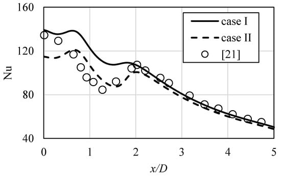
Figure 7.
The Nusselt number values at the impinged surface, in relation to applied flow conditions at the inlet. See Reference [21] to benchmark case results.
4.1. The Hydrodynamic and Thermal Boundary Layers
The absolute velocity values at various locations over the impinged surface, as well as the boundary layer thickness, were taken into consideration to identify further differences between the cases. In Figure 8, the velocity profiles obtained with “case I” are presented, while, in Figure 9, the velocity profiles obtained with “case II”. All particular values of the velocity are normalized with the bulk velocity ub. In addition, the boundary layer thickness is shown on both images, represented by the solid (Figure 8) and dotted (Figure 9) lines. It was calculated with assumption that it is limited to the distance, where the velocity reaches the 99% of the free stream velocity. In Figure 10, the additional close-up of the near wall area is shown to indicate the differences in the boundary layer thickness between two analyzed cases. The boundary layer thickness, as can be seen in Figure 8, Figure 9 and Figure 10, was growing along the x/D distance, starting from the stagnation point. However, the location of second maximum of Nusselt number, marked in Figure 10 as the vertical line, is characterized by the slight decrease in the boundary layer thickness. At the distances longer than x/D = 2.25, the height of the boundary layers stabilize, which indicates the occurrence of an already developed wall-jet.
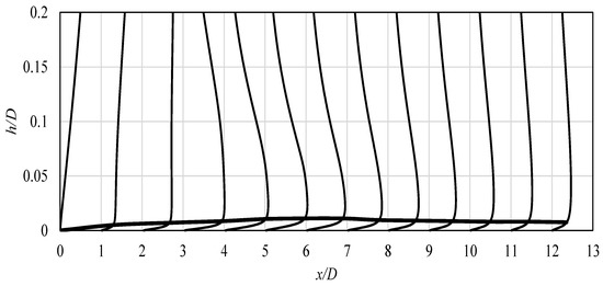
Figure 8.
Velocity profiles, normalized by the bulk velocity ub, obtained for “case I” (Table 3). Boundary layer thickness indicated by the thick solid line.
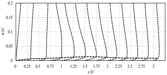
Figure 9.
Velocity profiles, normalized by the bulk velocity ub, obtained for “case II” (Table 3). Boundary layer thickness indicated by the dashed line.
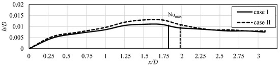
Figure 10.
Close-up of the boundary layer thickness obtained for “case I” and “case II” (Table 3). The second maxima of Nusselt number for both cases is also shown.
In Figure 11, the detailed velocity and turbulence intensity profiles are presented for selected distances x/D from the stagnation point. Therefore, they correspond to the velocity plots from Figure 8, Figure 9 and Figure 10. In Figure 11, the discrepancies of the presented variables values in the impinging jet can be noticed, in relation to the applied inlet profile. Some differences between the velocity profiles can be noticed; however, more important are the plots of the turbulence intensity (Figure 11b). As it can be seen, close to the stagnation point, the impact of the impinging jet is strong, as the difference in turbulent transport is significant. It vanishes at x/D of about 2, where the wall jet is developed. The characteristic maxima of turbulence intensity, visible in the last two plots in Figure 11b, located above the boundary layer, are connected with the characteristic big vortex that is clearly visible in Figure 12, where the global turbulence kinetic energy k field is shown for both analyzed cases. They also show approximate locations, where the overall maximum value of k was obtained for both cases. It is indicated by the white dots.
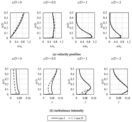
Figure 11.
The normalized velocity (a) and turbulence intensity (b) profiles in the boundary layer at the impinged surface for various values of non-dimensional x/D distance from the stagnation point.
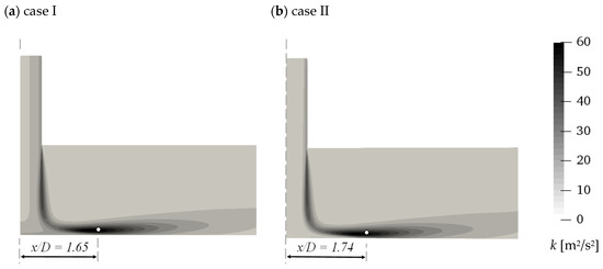
Figure 12.
The turbulence kinetic energy fields, obtained for “case I” (a) and “case II” (b). White dots indicate the turbulence kinetic energy global maxima.
In Figure 13, the temperature profiles at various x/D locations are presented, to provide also a data regarding the thermal boundary layer and its variation due to applied different inlet conditions. Temperature is presented as the non-dimensional value, divided by the mean inlet temperature, Tinlet. The differences are exhibited at all investigated locations until the wall jest was established, independent of the inlet parameters variations, as can be seen at the plot from location x/D = 2. With the increasing distance from the stagnation point, values at the surface for both cases increase, which corresponds to the formation of the boundary layer. It is worth noting that, near wall, the values obtained for “case II” are higher, while the tendency outside the boundary layer is opposite.
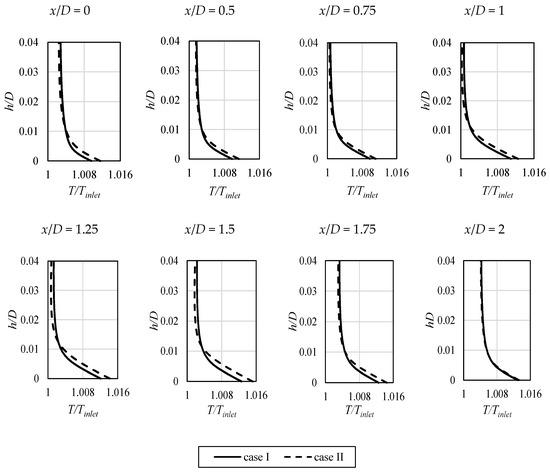
Figure 13.
The temperature profiles in the boundary layer at the impinged surface for various values of non-dimensional x/D distance from the stagnation point. Temperature values are presented in a non-dimensional way, being divided by the inlet temperature Tinlet.
4.2. Turbulence Characteristics of the Flow Near the Impinged Surface
In Figure 14, the corresponding results concerning the local values of turbulence kinetic energy rate
are shown. The reason to divide the values of turbulence kinetic energy by time was to maintain the consistency of results with data from Figure 15, presented later and concerning the budget of this variable. The values of turbulence kinetic energy rate
were obtained at first mesh cells above the heated and impinged wall, thus being located inside the boundary layer. The first conclusion that can be stated is connected with significantly lower values of the variable obtained for the “case II” before the wall-jet was generated (x/D ≈ 2). The first peak locations for both profiles corresponds to the location of the first peaks of the Nusselt number, shown in Figure 7. However, the second peaks of
are slightly away from the stagnation point, in comparison with the second peaks of the Nusselt number.
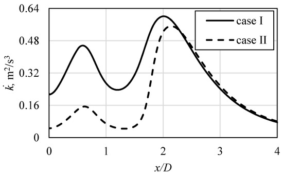
Figure 14.
The turbulence kinetic energy rate values at the first mesh node above the impinged surface, in relation to analyzed cases of the flow conditions at the inlet.
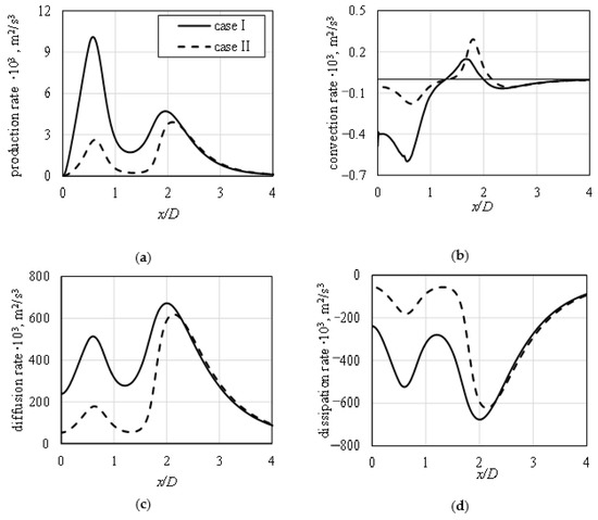
Figure 15.
Budget terms of the turbulence kinetic energy rate . The values are presented at the first mesh node above the impinged surface, in relation to applied flow conditions at the inlet. Production rate (a), convection rate (b), diffusion rate (c), and dissipation rate (d).
In general, the link between the values and behavior of
in relation to the heat transfer represented by the Nusselt number can be found. The highest values of
do not necessarily correspond to the highest values of Nusselt number; nevertheless, the rapid change of this variable, indicating creation of the highly turbulent zone, leads to increased heat transfer rates. As the mean turbulence kinetic energy rate
values, near impinged wall, exhibited the similarities between them and the Nusselt number distribution, its budget was also investigated, to gain deeper understanding of the jet impingement phenomenon. For the ζ-f model, the conservation equation for
takes the form of Equation (7). In Figure 15, all the budget terms of
are plotted, at the same location as the one used in the Figure 14. In general, higher values of all terms were obtained when “case I” was applied at the inlet. Two main terms that contribute to the budget of
are the diffusion rate, shown in Figure 15c, and the dissipation rate, balancing it, shown in Figure 15d. Their distribution is adequate to the distribution of turbulence kinetic energy rate from Figure 14, with two noticeable peaks, from which the second reaches higher values.
The production, in Figure 15a, and advection, in Figure 15b, rates do not contribute to the budget as strongly as the diffusion and dissipation because their values near-wall are very small in comparison with other two terms. The differences between both analyzed cases are clearly visible. While the “case I” profile applied at the inlet leads to high production rate of
at a distance from stagnation point equal to x/D ≈ 0.5 (approximate end of the stagnation zone), the “case II” does not cause such a big impact. It is surprising, despite the fact that the near-wall values of
imposed at the inlet (see Figure 6) are almost the same for both profiles, and the inlet pipe radius does not differ, being placed at the same radial distance from the stagnation point, equal to x/D = 0.5. Convective rate term has negative values near the stagnation point, and the change of its sign occurs close to the location of Nusselt number secondary maxima.
Another parameter that was compared at the near-wall locations was local enstrophy flux Ω, defined in Equation (13) on the basis of vorticity (velocity curl) [4], with enstrophy E definition shown in Equation (14):
Regions with high values of that variable are associated with those of high turbulence energy dissipation rate. As it can be seen in Figure 16, its values have also similar tendency as the Nusselt number. Similarly to the majority of the previously presented variables, the usage of “case I” led to higher values of Ω. For both profiles, the first peak of Ω was significantly higher than the second one. The reason is related to the fact that, at the location of x/D ≈ 0.5 (approximate end of the stagnation zone), the rapid change of direction of the impinging flow occurs. The second peaks of Ω are characterized by almost the same values; however, their locations slightly differ, as was in the case of the Nusselt number peaks. When the wall jet was formed, the differences between the two analyzed cases vanished.
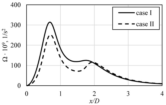
Figure 16.
The enstrophy flux, Ω, values at the first mesh node above the impinged surface, in relation to applied flow conditions at the inlet.
4.3. Turbulence Characteristics of the Impinging Jet Itself
The aforementioned data was related to the origin of the Nusselt number extrema outside the stagnation point. However, as it can be concluded from Figure 1, Figure 5 and Figure 7, the Nusselt number can also exhibit the maximum exactly at the stagnation point. The source of the intensive heat exchange at the stagnation point is still an open question [8,20,22]. It cannot be related to the turbulence production rate (as the values there are small, see Figure 14), and it is most often attributed to the influence of the inflow turbulence, which is the feature of the jet itself. The so-called potential core, in which the velocity remains almost constant in relation to the pipe exit, plays a major role in the heat transfer intensification at the stagnation point, as it includes the original characteristics of the inlet flow. The distance, denoted by h in Figure 4, between the stagnation point and the potential jet core termination, due to increased shear layers impact around the jet core, indicates how strongly it can affect the stagnation point. In Table 4, the difference in these distances between analyzed cases is shown, in a non-dimensional manner. The “case I” flow induced at the inlet kept its characteristic up to h equal to 0.555, which was closer to the stagnation point than that for the “case II”. As a result, the higher values of that point’s Nusselt number were obtained, as can be observed in Figure 7.
Table 4.
Non-dimensional distance h/D between the stagnation point and the potential jet core termination.
In Figure 17, Figure 18 and Figure 19, the additional data related to the potential core existence is shown. The evolution of the local profiles of velocity (Figure 17), turbulence intensity (Figure 18), and enstrophy (Figure 19) along the impinging jet is presented. When approaching the impinged surface, the distortion of all the profiles can be seen, with significant differences between the analyzed cases. “Case I”, which was characterized by higher turbulence levels in its core, prevails longer, whereas the velocity profile in Figure 17 is flatter close to the surface. In addition, the enstrophy plot at that location, shown in Figure 19, has lower values of its peak (which indicates the shear area). Its lower values mean that the jet is more resistant to the impact of the ambient, steady fluid.
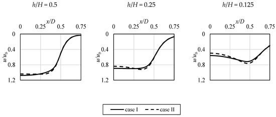
Figure 17.
Impinging jet absolute velocity profiles at various values of non-dimensional distance h/H above the impinged surface.
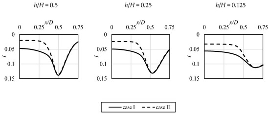
Figure 18.
Impinging jet turbulence intensity profiles at various values of non-dimensional distance h/H above the impinged surface.
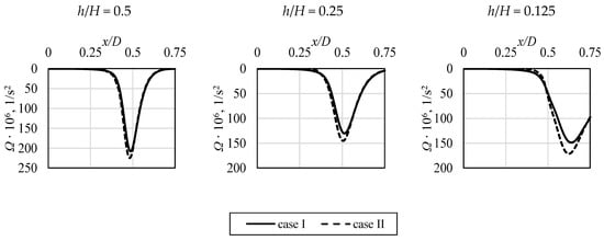
Figure 19.
Impinging jet enstrophy profiles at various values of non-dimensional distance h/H above the impinged surface.
5. Conclusions
The main goal of the following article was to analyze the jet impingement phenomenon and present the impact of the inlet flow conditions on the thermal performance at the impinged surface. It was related to the necessity of deeper understanding of the heat transfer processes that can occur in the heat exchanger [1], which was built on the basis of minigaps flow jet impingement. Numerical simulations were performed with the use of OpenFOAM (v2006) software. Turbulent conditions were numerically modeled, which was achieved by implementation of the RANS based on Hanjalic’s ζ-f model [14]. It was shown that, without the full definition of the conditions at the inlet, it is impossible to use particular results as the reference data, since the detailed analysis reveals significant discrepancies. Two types of conditions were considered, and both could be described as the developed flow. The mean velocities were the same, and the near-wall turbulence kinetic energy did not differ more than ~5%. However, as shown in the Results section, the conditions near the impinged wall (related to turbulence or, more generally, hydrodynamics of the flow) and at this wall (related to the thermal performance) differed significantly. A correlation between the values of turbulence kinetic energy rate
and the Nusselt number distribution was indicated. In addition, the analysis of the turbulence kinetic energy rate
budget near-wall, as well as the enstrophy flux distribution there, were presented. For all variables, clear discrepancies between utilized inlet conditions was shown.
Since many publications do not include detailed data regarding the applied inflow conditions, they should be carefully analyzed as the source of validation. Taking into account only some non-dimensional parameters, such as H/D or inlet Reynolds number, when choosing the reference, might not be enough sufficient for analysis the flows in micro-, mini-, or conventional channels. The research papers should also contain the data related to the turbulent properties of the issued jet because only velocity profiles are too general.
The authors also suggest including the flow profiles description close to the impinged surface (see Section 4.3) in the problem’s literature, as they are more significant than the ones at the nozzle/orifice exit and strongly influence the jet impingement phenomenon.
Author Contributions
Conceptualization, E.F.-W., T.K. and J.W.; methodology, T.K., E.F.-W., S.K. and S.G.; software, T.K.; validation, T.K., J.W., E.F.-W., S.K. and S.G.; formal analysis, T.K.; investigation, T.K. and S.G.; resources, T.K., J.W., E.F.-W. and S.G.; data curation, T.K.; writing—original draft preparation, E.F.-W. and T.K., and J.W.; writing—review and editing, T.K., J.W. and E.F.-W.; visualization, T.K., E.F.-W.; supervision, E.F.-W. and J.W.; project administration, T.K., E.F.-W. and J.W.; funding acquisition, T.K., J.W., E.F.-W. and S.G. All authors have read and agreed to the published version of the manuscript.
Funding
This research was funded by the Ministry of Science and Higher Education (for T. Kura, E. Fornalik-Wajs, S. Gurgul Grant AGH No. 16.16.210.476, while, for J. Wajs, Grant PG No. 034121).
Acknowledgments
This work was supported by the PLGrid Infrastructure.
Conflicts of Interest
The authors declare no conflict of interest.
Nomenclature
| Latin symbols | |
| a | thermal diffusivity, m2/s |
| C1 | ζ-f model constant, – |
| C′2 | ζ-f model constant, – |
| Cε1 | ζ-f model constant, – |
| Cε2 | ζ-f model constant, – |
| cp | specific heat, J/(kg K) |
| D | pipe/nozzle/orifice diameter, m |
| E | enstrophy, m2/s2 |
| f | elliptic relaxation of the ζ-f model, 1/s |
| G | turbulence production rate, m2/s3 |
| H | distance between the pipe/nozzle/orifice and impinged surface, m |
| H/D | jet to impinged surface ratio, – |
| h | variable representing a distance between the stagnation point and the potential jet core termination, m |
| h/D | non-dimensional distance between the stagnation point and the potential jet core termination |
| I | turbulence intensity, – |
| i | iteration, – |
| k | turbulence kinetic energy, m2/s2 |
| turbulence kinetic energy rate, m2/s3 | |
| L | turbulent length scale, 1/m |
| p | pressure, Pa |
| Sij | strain rate tensor, 1/s |
| T | temperature, K |
| u | velocity, m/s |
| ub | bulk velocity, m/s |
| uj | velocity components, m/s |
| u′ | velocity fluctuation, m/s |
| u* | friction velocity, m/s |
| root mean square of the fluctuation of the velocity normal to streamlines, m2/s2 | |
| x | radial variable from the stagnation point, m |
| x/D | non-dimensional distance along the heated surface, – |
| y | point to wall distance, m |
| y+ | dimensionless wall distance, – |
| Greek symbols | |
| α | heat transfer coefficient, W/(m2 K) |
| αef | effective heat transfer coefficient, W/(m2 K) |
| ε | dissipation of the turbulence kinetic energy rate, m2/s3 |
| ζ | normalized by k, – |
| Θ | mean temperature, K |
| θ | temperature fluctuation, K |
| λ | thermal conductivity of the fluid, W/(m K) |
| μ | dynamic viscosity, Pa s |
| ν | kinematic viscosity, m2/s |
| νt | eddy viscosity, m2/s |
| ρ | density, kg/m3 |
| τ | turbulent time scale, 1/s |
| σε | ζ-f model constant, – |
| σk | ζ-f model constant, – |
| σζ | ζ-f model constant, – |
| Ω | enstrophy flux, 1/s2 |
References
- Kura, T.; Fornalik-Wajs, E.; Wajs, J. Thermal and hydraulic phenomena in boundary layer of minijets impingement on curved surfaces. Arch.Thermodyn. 2018, 39, 147–166. [Google Scholar]
- Yamagami, S. Surface Orientation Effect on Local Heat Transfer by Round Water Jet Impingement. Flow Turbul. Combust. 2019, 102, 485–496. [Google Scholar] [CrossRef]
- Clayton, D.J.; Jones, W.P. Large Eddy Simulation of Impinging Jets in a Confined Flow. Flow Turbul. Combust. 2006, 77, 127–146. [Google Scholar] [CrossRef]
- OpenFOAM Extended Code Guide. Available online: https://www.openfoam.com/documentation/guides/latest/doc/ (accessed on 15 November 2020).
- Grenson, P.; Léon, O.; Reulet, P.; Aupoix, B. Investigation of an impinging heated jet for a small nozzle-to-plate distance and high Reynolds number: An extensive experimental approach. Int. J. Heat Mass Transf. 2016, 102, 801–815. [Google Scholar] [CrossRef][Green Version]
- Harekrishna, Y.; Agrawal, A. Effect of vortical structures on velocity and turbulent fields in the near region of an impinging turbulent jet. Phys. Fluids 2018, 30, 035107. [Google Scholar]
- Lee, J.; Lee, S.-J. Stagnation region heat transfer of a turbulent axisymmetric jet impingement. Exp. Heat Transf. 1999, 12, 137–156. [Google Scholar] [CrossRef]
- O’Donovan, T.S.; Murray, D.B. Jet impingement heat transfer—Part 1: Mean and root-mean-square heat transfer and velocity distributions. Int. J. Heat Mass Transf. 2007, 50, 3291–3301. [Google Scholar] [CrossRef]
- Garimella, S.V.; Nenaydykh, B. Nozzle-geometry effects in liquid jet impingement heat transfer. Intern Int. J. Heat Mass Transf. 1996, 39, 2915–2923. [Google Scholar] [CrossRef]
- Lee, D.H.; Song, J.; Jo, M.C. The effects of nozzle diameter on impinging jet heat transfer and fluid flow. J. Heat Transf. 2004, 126, 554–557. [Google Scholar] [CrossRef]
- Royne, A.; Dey, C.J. Effect of nozzle geometry on pressure drop and heat transfer in submerged jet arrays. Int. J. Heat Mass Transf. 2006, 49, 800–804. [Google Scholar] [CrossRef]
- Ping, Z.; Liang-chun, Y.; Jie-min, Z.; Ying, Y. Analysis of disagreement between numerically predicted and experimental heat transfer data of impinging jet. J. Cent. South Univ. 2006, 13, 486–490. [Google Scholar]
- Kenjeres, S.; Gunarjo, S.B.; Hanjalic, K. Contribution to elliptic relaxation modelling of turbulent natural and mixed convection. Int. J. Heat Fluid Flow 2005, 26, 569–586. [Google Scholar] [CrossRef]
- Hanjalic, K.; Popovac, M.; Hadziabdic, M. A robust near-wall elliptic-relaxation eddy-viscosity turbulence model for CFD. Int. J. Heat Fluid Flow 2004, 25, 1047–1051. [Google Scholar] [CrossRef]
- Kura, T.; Fornalik-Wajs, E.; Wajs, J.; Kenjeres, S. Turbulence models impact on the flow and thermal analyses of jet impingement. MATEC Web Conf. 2018, 240, 01016. [Google Scholar] [CrossRef]
- Kura, T.; Fornalik-Wajs, E.; Wajs, J.; Kenjeres, S. Local Nusselt number evaluation in the case of jet impingement. J. Phys. Conf. Ser. 2018, 1101, 012018. [Google Scholar] [CrossRef]
- Popovac, M.; Hanjalic, K. Compound wall treatment for rans computation of complex turbulent flows and heat transfer. Flow Turbul. Combust. 2007, 78, 177–202. [Google Scholar] [CrossRef]
- Cooper, D.; Jackson, D.C.; Launder, B.E.; Liao, G.X. Impinging jet studi es for turbulence model assessment: Part 1, flow field experiments. Int. J. Heat Mass Transf. 1993, 36, 2675–2684. [Google Scholar] [CrossRef]
- Behnia, M.; Parneix, S.; Durbin, P.A. Prediction of heat transfer in an axisymmetric turbulent jet impinging on a flat plate. Int. J. Heat Mass Transf. 1998, 41, 1845–1855. [Google Scholar] [CrossRef]
- Behnia, M.; Parneix, S.; Shabany, Y.; Durbin, P.A. Numerical study of turbulent heat transfer in confined and unconfined impinging jets. Int. J. Heat Fluid Flow 1999, 20, 1–9. [Google Scholar] [CrossRef]
- Yan, X. A preheated-Wall Transient Method Using Liquid Crystals for the Measurement of Heat Transfer on External Surfaces and in Ducts. Ph.D. Thesis, University of California, Davis, CA, USA, 1993. [Google Scholar]
- Baughn, J.W.; Shimizu, S. Heat transfer measurements from a surface with uniform heat flux and an impinging jet. J. Heat Transf. 1989, 111, 1096–1098. [Google Scholar] [CrossRef]
Publisher’s Note: MDPI stays neutral with regard to jurisdictional claims in published maps and institutional affiliations. |
© 2020 by the authors. Licensee MDPI, Basel, Switzerland. This article is an open access article distributed under the terms and conditions of the Creative Commons Attribution (CC BY) license (http://creativecommons.org/licenses/by/4.0/).