Abstract
In this work, the real-time mathematical models of electromechanical power systems with semiconductor converters based on the author’s method of the average voltages in the integration step are described. As well as the theoretical basics of the method, the algebraization algorithm of differential equations on a time quantum is described. This time quantum in the hybrid model is synchronized with the time quanta of signal samples of the physical part of the model. In the hybrid model, only algebraic equations of electromechanical power systems are present. Software and technical applications of the hybrid models of energy-generating blocks for selected thermal and nuclear power plants are described. In the process curve courses obtained and projected in this paper, the author’s hybrid models are illustrated. In the existing models, the nonlinearity of the electric machines and the semiconductor converters are taken into account. The numerical stability of the method of average voltages in integration step—in the sense of the resistance to computer calculation disturbances—is proven.
1. Introduction
There are two subsystems in modern electromechanical systems: the energy conversion system (power scheme) and information conversion system (control, regulation and automatic circuits). The authors have accumulated many years of experience in the study of electromechanical systems in a hybrid environment, in which the power part is a virtual mathematical model and the automatic control system is a real physical object. Today, this approach corresponds to hardware-in-the-loop technologies, which are described in [1,2,3,4,5]. The computer application of the power scheme must work in a real-time mode (real-time model) and must be stable to the numerical disturbances caused by the limit of real number digits in the computer application. The authors dealt with numerical stability problems during the implementation of their projects; additionally, these problems were considered in [4,5,6]. The author’s method of average voltages in the integration step [7] is effective in providing numerical stability for models of power schemes with electrical circuits. Their application has provided numerical stability in the described projects during an unlimited period of hybrid model working, which could not be provided by using classical explicit and implicit methods (Runge–Kutta, Adams, trapezoids, etc.). The author’s method is also effective in providing high performance, which was proven in [8].
This article deals with models of the power circuits of electromechanical systems, which are based on the method of average voltages in the integration step and its computer application in hybrid models of power generation systems based on the example of selected nuclear and thermal power plants; furthermore, the work presents a demonstration of the processes which are obtained for the hybrid models developed by the authors and an explanation of the method’s stability.
In addition, the proposed method solves a problem in the time domain. The method algebraizes differential equations of electromechanical systems’ power circuits within numerical quanta of time, which are synchronized in the hybrid models with signal quanta of time from a physical object. Other methods of algebraization are possible; for example, in the frequency domain [9]. However, in our opinion, using the time domain with a one-step algebraization method is optimal for real-time models of electromechanical systems with electric machine nonlinearities and semiconductor converters. Our opinion is the same as that of the authors in [9,10].
2. Method Description
Electromechanical systems are described by differential and algebraic equations, which are basically nonlinear. Numerical methods are used for solving equations, namely for the algebraization of differential equations in the integration step. Disturbances occur during numerical algebraization, which are caused by number rounding in computer applications (round-off error). This leads to numerical instability during multiple numerical iterations. This problem appears especially in hybrid models, in which the mathematical model works in a real-time mode for a long period. The authors highlight two factors which cause these problems.
The first factor is that a system of equations contains variables, which are simultaneous in differential and algebraic equations. An example is an electrical scheme, which is simultaneously described by Kirchhoff’s first and second laws. The algebraization of differential equations by explicit methods (for example, Euler or Runge–Kutta) causes error accumulation during the solving of algebraic equations (the sum of the calculated values of currents at the system nodes in multiple calculations is equal to the error). The algebraization of differential equations by implicit methods causes a numerical disturbance during the solving of differential equations (the sum of the calculated values of the voltages in the system circuits in multiple calculations is equal to the error).
The second factor is that variables variation in the integration step are different in their characters. For example, in the case of a series connection of inductance and capacitors, the capacitor voltage is described by a series, which has an order higher than the order of the current series. The same situation can be noted for the rotor speed and rotor angle of an electric machine. Thus, using the same approach to integrate these variables is incorrect and therefore generates errors.
Here, we propose the application of the method of average voltages in the integration step for the algebraization of equations; this process was first described in [7] and used in the projects presented in [11,12]. The method is robust to the numerical disturbances described above.
The general interpretation of the method is as follows:
The equations which describe electromechanical systems (power conversion systems) are written as follows:
The initial conditions for the integration step are written as follows:
In Equations (1) and (2), x is the argument (mostly time), is the vector of functions, is the vector of derivative functions, K is the coefficient matrix for the algebraic equations system, and is the vector of absolute values of the algebraic equation system.
The vector differential Equation (1) is written after integration as
The name of this integration is the title of the method: “the method of average values of variables in the integration step”. The variables were the voltages for the branch of the electrical circuits in the first applications of the method. Thus, the method was titled “the method of average voltages in the integration step”.
Assuming that the vector is represented as a truncated Taylor series in the integration step,
and substituting this expression in Equation (4), a system of vector equations is written as
where is the vector of variables at the end of the integration step; is the nonlinear function of the vector (for example, the dependence of the value of the magnetic flux on the magnetizing current at saturation of the magnetic circuit); R is the matrix and is the vector of average parameters in the integration step; and the expressions for and R are functions of the parameters of the Taylor series and Equation (1).
The number of members of the Taylor series m determines the order of the method, namely the method of average voltages in the integration step of the first, second, … m-th order. In our experience, the optimal version is the second-order method.
The presented description of the method is general. The method application for a specific power system is described as follows.
The equation for an electric branch which contains an electromotive force source, inductance, capacitance and resistance is written as
where u, e, uR, uC, uL are the instantaneous values of applied voltage, electromotive force, and voltages on appropriate branch elements, respectively, t0 is the time value at the beginning of integration step, and Δt is the integration step value.
Instantaneous values of voltages on the resistor and capacitor are represented as
where uR0, uC0 are values of voltages at the beginning of the integration step; and ΔuR, ΔuC are increments of voltages in the integration step, which are represented in the form:
where , are the k-order derivatives of voltages on the resistor and capacitor at the beginning of the integration step.
Taking into consideration the known dependencies between the voltages and current for branch elements, on the basis of Equations (8)–(10), the following equation was obtained, in which the unknowns are the branch’s current at the end of integration step i1 and the average voltage applied to the branch U [8]:
where i0 is the current value at the beginning of the integration step; L0, L1 are the branch inductances at the beginning and at the end of the integration step; m is the order of the polynomial by which a current is described in an integration step (the order of method); and , are average values of the applied voltage and electromotive force in the integration step, respectively.
As noted above, the second-order method (m = 2) is optimal from our project experience. In this case, the equation is written as
The currents at the end of the integration step i1 are determined from Equation (12). The voltage of the capacitor at the end of integration step (for the second-order method) is written as
It should be noted that components of Equations (11)–(13), which include capacitance, are zero in the case of the absence of capacitance in the circuit branch. In other words, we must substitute voltage Uc0 for zero and capacitance for infinity in these equations to exclude capacitance. The inductances L1, L0 are zero in the case of the absence of inductance. This means that the method is applicable to any circuit, which includes any combination of R, L, and C elements.
Equations (12) and (13) should be supplemented by Equation (7) for the nodes.
Equations (12) and (13) are the result of the algebraization of differential equations in the integration step. Numerical stability is ensured by solving equations in which the algebraic sum of voltages is zero at the beginning of the integration step (Kirchhoff’s second law), and the sum of currents is zero at the end of the integration step (Kirchhoff’s first law). Stability is absent when using classical methods, in which there are no explicit equations for the sum of currents equal to zero (explicit methods), or for a sum of voltages equal to zero (implicit methods). In addition, the contradictions in the integration of current and voltage for the capacitance, which have different steepnesses in the integration step, and which also affect the numerical stability, are eliminated. The model of the system was formed on the basis of the multipolar theory applied in [13], where the description of electric machines and semiconductor converters was applied, taking into account their nonlinearities.
Each element of the power scheme of the electromechanical system was represented by a multipole and is described by the vector equations:
where is the vector of potentials of the multipole’s external poles; is the vector of currents of the multipole’s external branches; and , are the matrix of coefficients and the vector of the absolute values, respectively.
According to Kirchhoff’s first law, the equation is written as
where is the incidence matrix, which determines the method of connecting the outer branches of multipoles to the independent nodes of an electrical circuit and describes the topology of the power circuit; and L is the quantity of elements in the power system. The incidence matrices set the relation between the potentials of the multipole’s external poles and potentials of independent nodes (for averaging integration step values):
From Equations (14)–(16), the following matrix algebraic equation for the average values in the integration step of the potentials of independent nodes is obtained,
with its coefficients being defined after coefficients of matrix Equation (14) for each element, and after the elements’ incidence matrices: , .
The average values for an integration step of an independent system’s nodes potentials were obtained from Equation (17). The average values for the integration step of an external pole’s potentials for every element are obtained from Equation (16) and the currents of the external branches at the end of the integration step were calculated from Equation (14). The average values for the integration step of voltages on capacitors were determined from Equation (13).
3. Mathematical Models of Elements
The principles of the mathematical model’s construction for elements of an electromechanical system’s power scheme are illustrated by the example of the mathematical model of a synchronous machine. The mathematical model of the synchronous machine is developed in phase coordinates and takes into consideration the non-linearity of the magnetic circuit characteristics and the influence of the rotor damper system. The calculation scheme of a synchronous machine as an eight-pole is shown in Figure 1. The damping system of the synchronous machine is represented by two short-circuited windings oriented on axes d and q.
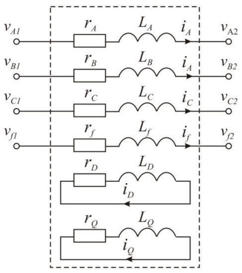
Figure 1.
Calculation scheme of the synchronous machine.
According to Equation (11), the vector equations for external (stator and excitation windings) and internal (damping) circuits for the calculation scheme on Figure 1 are written as
where , are the vectors of the external pole potentials; , are the vectors of the currents in the internal and external branches; , are the vectors of flux linkages; are the matrices of the resistances of stator winding and excitation winding; and are the matrices of the resistances of the damping winding. Indexes 0 and 1 indicate the value of the variable at the beginning and at the end of the integration step.
The flux linkage changes of the external and internal circuit of the synchronous machine on the integration step are as follows:
where is the matrix of the self and mutual inductances of the external circuit, in which the diagonal elements are the self-inductances of the stator and field windings, and all the others are the mutual inductances of appropriate windings; are the matrices of the mutual inductances between the external and internal circuits; and is the matrix of the damper system inductances.
Equations (20) and (21) describe the flux linkage changes for the integration step of the external and internal circuit, which were caused by the changes of the current in the integration step and electromagnetic parameter changes caused by rotor rotation.
Equations (18) and (19), using Equations (20) and (21), are written as
where is the matrix of the step resistance of the internal circuit.
Equation (23) is an algebraic equation used for the determination of the internal circuit’s current in the integration step. Equation (22) using Equation (23) is written as Equation (14) for a synchronous machine:
where , are the matrix of coefficients and the vector of the absolute values, respectively; is the step electromotive force determined by the initial conditions; , , are the matrices of the step resistances of the external circuits at the beginning and end of the step; gives the vectors of the external pole’s potentials; is the vector of the currents in the internal and external branches.
Equation (24) is an algebraic equation used to determine currents of the external circuits based on external pole’s potentials.
The received equations for electric circuits are supplemented by the equation of motion:
where M is the electromagnetic torque; MS is the external mechanical torque on the shaft, which is calculated by mathematical model of drive; J is the moment of inertia of the unit; and ω is the rotor speed.
Equations (23)–(25) form the mathematical model of the synchronous machine.
The mathematical models of other elements are formed as multipoles, such as the mathematical model of the synchronous machine.
The semiconductor switches are presented as a resistance with a low value in the “on” state and a high value in the “off” state. The switch turns off at the time its current crosses zero from the positive to the negative value (these times are calculated by solving algebraic equations for the current of the commutating switch). The switch “turn-on” times are defined from logical equations on the basis of the information received from the control system.
4. Application
The described method was used by authors in many projects, particularly in digital diagnostic complexes for brushless excitation systems for the Kursk Nuclear Power Plant (Russia), the South-Ukrainian Nuclear Power Plant, as well as for static excitation systems for turbogenerators of thermal power plants; in particular, the Burshtyn Thermal Power Plant (Ukraine).
The examples of the application of a real-time computer model of a power scheme for a power generation system in conjunction with a physical generator control system (hardware-in-the-loop structure) are described below. This “hybrid” system is used to test, diagnose, and debug the physical control system of the generator before it is connected to the generator, as well as periodically during its operation for prevention purposes. The structural–functional scheme of the system is shown in Figure 2.
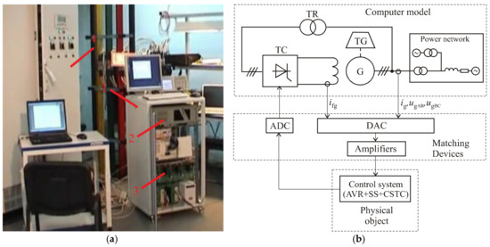
Figure 2.
Appearance (a) and functional scheme (b) of the hybrid model for a power generation system with the static excitation system of synchronous generator 1: computer model of power scheme, 2: industrial computer, 3: matching elements (amplifiers), 4: excitation system of synchronous generator.
The power scheme, implemented in the computer model, contains a synchronous generator G (rated power Pn = 63 MW; rated voltage and current Un = 10,750 V, In = 3980 A) with a semiconductor self-excitation system, in which the excitation current is regulated by thyristor converter TC. The thyristor converter is supplied by the synchronous generator’s output voltage through the transformer. The generator is driven by the turbine TG with the speed control system. The load of the generator is the model of the Power Network consisting of the parallel-working generators of the power plant and the power line with the equivalent electromotive force.
The thyristor converter is controlled by signals from the real control system (excitation controller) including the automatic excitation control system with the voltage regulator (AVR) and the system stabilizer (SS), as well as the thyristor converter control system (CSTC). The following signals are emitted from the computer model into the excitation controller: the generator’s output linear voltages ugAB, ugBC, the generator’s stator current ig, and the generator’s excitation current ifg. The control voltage for the thyristor converter is sent to the computer model from the excitation controller. The matching devices provide the interconnection between the computer and the real part of the hybrid model. Their functions are analog-to-digital and digital-to-analog conversion (the analog excitation controller is used), as well as the signal’s level matching and power amplification. In particular, the nominal values of the signals of the generator’s voltages and stator current on the inputs of the real excitation controller must be 100 V and 5 A, accordingly. The matching devices provide the work conditions for the excitation controller, in a similar manner to the power plant.
The research results in the form of the experimental oscillograms of the generator excitation current If, the effective value of the generator terminal voltage UT, the reference value of the generator terminal voltage Uref, and the active and reactive power at the generator’s output Pg, Qg are shown in Figure 3, Figure 4 and Figure 5. Oscillograms were derived from the physical excitation system co-operating with the excitation system’s software. All values on the oscillograms are given in relative units.
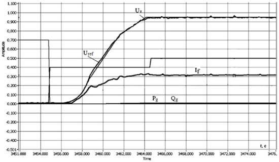
Figure 3.
The mode of the initial excitation of the generator without load.
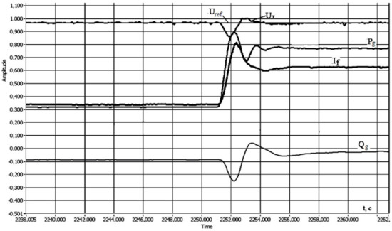
Figure 4.
The mode of an abrupt loading of the generator by active power.
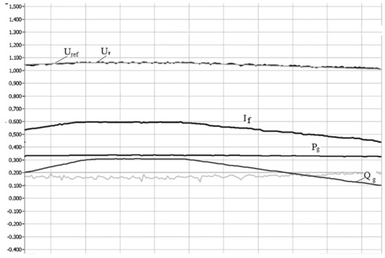
Figure 5.
The oscillogram for the mode of the generator’s reactive power regulation by changing the generator’s voltage setting (the time scale is 2 s).
The experimental oscillogram for the mode of the initial excitation of the non-loaded generator (the generator was disconnected from the network) is shown in Figure 3.
The automatic voltage regulator provides the generator terminal voltage, increasing in accordance with the set point signal (reference), which varies according to the prescribed law.
The research results for the case of an abrupt loading of the generator by active power are shown in Figure 4. Under this loading, there was a dynamic drop of voltage by 0.1 nominal value. These experiments made it possible to adjust the generator control system.
The oscillogram obtained for the mode of the generator’s reactive power regulation by changing the generator’s voltage setting on the physical excitation system is shown in Figure 5.
In the case of an increase of the generator voltage set point, the magnitudes of the excitation current and the reactive power that the generator generates into the power network increase (a positive signal of reactive power means the mode of return of power to the network). In the case of a decrease of the generator voltage set point, the generator’s excitation current and the reactive power are reduced. With a significant reduction of the excitation current, the generator switches to reactive power consumption from the power network. A significant consumption of reactive power by a synchronous turbogenerator is not allowed due to the overheating of the tooth areas of the rotor. Therefore, in automatic excitation controllers, a minimum excitation limit is provided in order to prevent this mode.
Another hybrid model was implemented as part of a project to diagnose a brushless excitation system for a turbogenerator with power of 1000 MW, which is operated, in particular, at nuclear power plants in Ukraine and Russia. The appearance of the digital diagnostic complex and the functional diagram of the hybrid model combining a real automatic excitation controller and a computer model of the power generation system are shown in Figure 6.
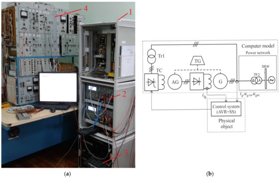
Figure 6.
Appearance (a) and functional scheme (b) of the hybrid model for a power generation system with a brushless excitation system for the turbogenerator. 1: computer model of power scheme, 2: matching elements (amplifiers), 3: industrial computer, 4: excitation controller.
The power scheme contains the main synchronous generator (G), auxiliary generator (brushless synchronous machine (AG)), turbine (TG), input transformer (TR1) of the main generator excitation system, generator transformers (TR2), and thyristor converter (TC). The main generator is excited by a brushless exciter (AG); its excitation current is regulated by a thyristor converter.
The signals of the generator terminal voltage (ugAB, ugBC), the generator stator current (ig), the generator excitation current (ifg) are sent from the computer model to the excitation controller. The control voltage of the controlled rectifier (thyristor converter (TC) in the computer model) is applied from the real excitation controller.
The oscillogram for the mode of the repeated short circuits (one and two-phase) in the power network, which are obtained in the hybrid model (Figure 6) with the physical excitation controller of the turbogenerator, which is operated at the South-Ukrainian Nuclear Power Plant, is shown in Figure 7.
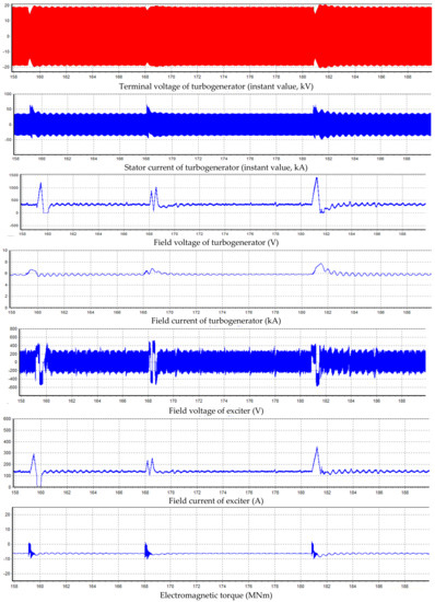
Figure 7.
The oscillogram for the mode of the repeated short circuits (one and two-phase) in the power network of the power generation system with a brushless excitation system for the turbogenerator.
The short-circuit mode is accompanied by a resynchronization of the generator, during which oscillations occur due to changes in the load angle. The basic coordinates set the generator (stator current, excitation current, electromagnetic torque) depending on the moment of occurrence of the short circuit in relation to the voltage phase angle of the power network. The excitation system forces the excitation voltage and excitation current in the case of a short circuit to increase the generator’s electromagnetic torque to avoid the loss of synchronism caused by the increasing of the rotor speed and load angle. The developed model allows us to estimate the magnitude of the oscillations of the generator’s electromagnetic torque in short-circuit modes, and therefore to evaluate the effect of these modes on the turbine.
5. Conclusions
The method of average voltages in the integration step provides numerical stability for hybrid real-time models and ensures the analytical–numerical algebraization of differential equations of electromechanical power circuits on time quanta, which are synchronized with time quanta of control system signals. This is important for the operation of hybrid models for an unlimited period of time.
The method is applicable for systems for which variables are described in the integration step by polynomials of a different order; for example, the voltage for the capacitance and current in a branch with series-connected inductance and capacitance, as well as the rotor speed and angle in electric machines.
Mathematical models of elements are represented as multipoles, providing generality for electromechanical systems models. The use of multipolar models makes it possible to parallelize the calculation and increase the speed of performance.
The developed real-time models of the power schemes of nuclear and thermal power plant generator blocks work in conjunction with the real excitation control system of generators during diagnosis and testing. In particular, the use of a real-time model for the generator blocks allows us to test and tune-up the real automatic excitation controllers of generators at power plants, as well as to train service staff.
The use of the author’s method of average voltage in the integration step enables to increase the numerical stability and performance of models and ensures their continuous operation in a real-time mode in combination with physical objects.
The models provide high-precision, instantaneous modeling with an error of less than 10%, which is determined by the precision of the identification of power scheme parameters. This is ensured by the high completeness of the description of electric machines and converters, taking their nonlinearity into account.
Author Contributions
Conceptualization, O.P.; methodology, O.P. and A.K.; software, A.K.; validation, O.P., A.K. and M.S.; formal analysis, M.S.; investigation, O.P., A.K. and M.S.; resources, M.S.; data curation, M.S.; writing—original draft preparation, A.K. and M.S.; writing—review and editing, O.P. and A.K.; visualization, M.S. All authors have read and agreed to the published version of the manuscript.
Funding
This research received no external funding.
Conflicts of Interest
The authors declare no conflict of interest.
References
- Benigni, A.; Monti, A. A parallel approach to real-time simulation of power electronics systems. IEEE Trans. Power Electron. 2015, 30, 5192–5206. [Google Scholar] [CrossRef]
- Faruque, M.O.; Strasser, T.; Lauss, G.; Jalili-Marandi, V.; Forsyth, P.; Dufour, C.; Dinavahi, V.; Monti, A.; Kotsampopoulos, P.; Martinez, J.A.; et al. Real-Time Simulation Technologies for Power Systems Design, Testing, and Analysis. IEEE Power Energy Technol. Syst. J. 2015, 2, 63–73. [Google Scholar] [CrossRef]
- Iacchetti, M.F.; Perini, R.; Carmeli, M.S.; Castelli-Dezza, F.; Bressan, N. Numerical Integration of ODEs in Real-Time Systems Like State Observers: Stability Aspect. IEEE Trans. Ind. Appl. 2012, 48, 132–141. [Google Scholar] [CrossRef]
- Parma, G.G.; Dinavahi, V. Real-time digital hardware simulation of power electronics and drives. IEEE Trans. Power Deliv. 2007, 22, 1235–1246. [Google Scholar] [CrossRef]
- Vilsen, S.A.; F⊘re, M.; S⊘rensen, A.J. Numerical models in real-time hybrid model testing of slender marine systems. In Proceedings of the OCEANS 2017—Anchorage, Anchorage, AK, USA, 18–21 September 2017; pp. 1–6. [Google Scholar]
- Ufa, R.A.; Vasilev, A.S.; Suvorov, A.A. Development of hybrid model of B2B HVDC. In Proceedings of the 2017 International Conference on Industrial Engineering, Applications and Manufacturing (ICIEAM), St. Petersburg, Russia, 16–19 May 2017; pp. 1–5. [Google Scholar]
- Plakhtyna, O. Numerical One-Step Method of Electric Circuits Analysis and Its Application in Electromechanical Tasks; Kharkivskyi Politekhnichnyi Instytut: Kharkiv, Ukraine, 2008; Volume 30, pp. 223–225. (In Ukrainian) [Google Scholar]
- Płachtyna, O.; Kłosowski, Z.; Żarnowski, R. Efficiency evaluation of average-step voltages method comparing to clasical methods of numerical integration applied to mathematical models of eletrical circuits. Prace Nauk. Politech. Śl. Elektr. 2012, 217, 121–133. (In Polish) [Google Scholar]
- Naredo, J.L.; Mahseredjian, J.; Kocar, I.; Gutierrez-Robles, J.A.; Martinez-Velasco, J.A. Chapter 3: Frequency domain aspects of electromagnetic transient analysis. In Transient Analysis of Power Systems: Solution Techniques, Tools and Applications, 1st ed.; Martinez-Velasco, J.A., Ed.; Wiley-IEEE Press: Hoboken, NJ, USA, 2015; pp. 33–71. [Google Scholar]
- Dufour, C.; Belanger, J. Chapter 4: Real-time simulation technologies in engineering. In Transient Analysis of Power Systems: Solution Techniques, Tools and Applications, 1st ed.; Martinez-Velasco, J.A., Ed.; Wiley-IEEE Press: Hoboken, NJ, USA, 2015; pp. 72–99. [Google Scholar]
- Plachtyna, O.; Kutsyk, A. A hybrid model of the electrical power generation system. In Proceedings of the 2016 10th International Conference on Compatibility, Power Electronics and Power Engineering (CPE-POWERENG), Bydgoszcz, Poland, 29 June–1 July 2016; pp. 16–20. [Google Scholar]
- Kłosowski, Z.; Cieślik, S. Real-time simulation of power conversion in doubly fed induction machine. Energies 2020, 13, 673. [Google Scholar] [CrossRef]
- Ye, P. Mathematical Modeling of Electromechanical Systems with Semiconductor Converters; Vyshcha Shkola: Kyiv, Ukraine, 1986; 161p. (In Russian) [Google Scholar]
© 2020 by the authors. Licensee MDPI, Basel, Switzerland. This article is an open access article distributed under the terms and conditions of the Creative Commons Attribution (CC BY) license (http://creativecommons.org/licenses/by/4.0/).