Abstract
Electric vehicles (EVs) have attracted growing attention in recent years. However, most existing research has not utilized actual traffic data and has not considered real psychological decision-making of owners in analyzing the charging demand. On this basis, an urban EV fast-charging demand forecasting model based on a data-driven approach and human decision-making behavior is presented in this paper. In this methodology, Didi ride-hailing order trajectory data are firstly taken as the original dataset. Through data mining and fusion technology, the regenerated data and rules of traffic operation are obtained. Then, the single EV model with driving and charging behavior parameters is established. Furthermore, a human behavior decision-making model based on Regret Theory is introduced, which comprises the utility of time consumption and charging cost to plan driving paths and recommend fast-charging stations for vehicles. The rules obtained from data mining together with established models are combined to construct the ‘Electric Vehicles–Power Grid–Traffic Network’ fusion architecture. At last, the actual urban traffic network in Nanjing is selected as an example to design the fast-charging demand load experiments in different scenarios. The results demonstrate that this proposed model is able to effectively predict the spatio-temporal distribution characteristics of urban fast-charging demands, and it more realistically simulates the decision-making psychology of owners’ charging behavior.
1. Introduction
As a cleaner means of transportation that is low-carbon and environmentally friendly, electric vehicles (EVs) can not only reduce greenhouse gas emissions [1,2], but they also improve country strategies to secure energy [3]. Moreover, EVs will introduce new connections and synergies between transportation networks and the power grid [4]. They will gradually replace traditional fuel vehicles and become an important trend in the future development of the automotive industry.
According to the plan of energy conservation and development for new energy automobile industry (2012–2020) issued by the State Council of China in 2012 [5], the total number of EVs in China is expected to be 5 million, the number of charging stations is about 12,000, and the number of charging devices will reach 4.5 million by 2020. As of the end of 2018, the number of new-energy vehicles in China rose 70% to 2.61 million, accounting for 1.09% of the total number of vehicles. There were 331,000 public charging piles and 477,000 private charging piles in 2018, an increase of 74.2% over the same period in 2017 [6].
However, the driving and charging behaviors of numerous EVs in urban internal networks are bound to interact with the energy and information generated by the traffic network and power grid [7,8]. The residents’ trip rule, urban road network structure and charging facility distribution affect the vehicle driving distribution and charging selection, whereas the vehicle battery parameters, driving path plan and human decision-making behavior also affect the degree of traffic network obstruction and the power grid operation state [9,10,11,12]. Therefore, accurate prediction of EV charging demand and reasonable fast-charging station (FCS) recommendations are the premise of realizing compatibility between EVs and the power grid along with the transportation network.
At present, various studies have developed EV charging demand models from the aspect of cooperation between EVs, the transportation system and power system all together. Hence, in [13,14], an origin destination (OD) matrix analysis method was utilized to track the all-weather driving trajectory of EVs and to predict the charging load distribution of the regional electricity grid as well as the flow status of road networks through vehicle traffic trip demands. Several studies [15,16,17] introduced Traffic Trip Chain and Markov Decision Chain to simulate the dynamic driving behavior and random charging behavior of EVs, established a dynamic EV charging demand prediction model and evaluated the congestion degree on the distribution network and traffic network caused by large-scale aggregation charging. In addition, researchers [18,19] adopted a microscopic traffic model to depict the dynamic characteristics and electrical state of EVs in the joint simulation system of transportation electrification, and they predicted the evolution trend of vehicle traffic demand and charging demand. Further, traffic nodes and electricity nodes in heterogeneous physical space were mapped to networks in studies [20,21]. The driving behavior in traffic topology and charging behavior in distribution network topology were coupled to network modeling, and a ‘vehicle–road–network’ integration system was constructed. This system was capable of analyzing the charging demand distribution, traffic flow status and effectiveness of implementing a charging scheduling strategy.
Although the above works comprehensively considered traffic factors and electricity factors to describe the dynamic driving process and random charging behavior of EVs, the established charging demand models were consistent with the characteristics of EV movable load. All of them were analyzed from the aspect of simulation modeling without using measured data for theoretical verification. However, it is worth noting that model analysis based on data-driven technology is closer to the actual charging load operation.
Accordingly, in [22,23,24,25], the taxi driving trajectory was taken as original data, and floating vehicle acquisition technology was adopted for data mining and behavior modeling. These researchers [22,23] exploited the GPS trajectory positioning data of Beijing taxis to mine the vehicle trip rules and clustering distribution characteristics, thereby predicting the charging demand and addressing the siting and sizing of urban fast-charging stations. Ashtari et al. [24] statistically analyzed GPS driving record data of Canadian taxis all day long. They assumed that EVs and fuel vehicles had the same driving habits, and they constructed a stochastic dynamic model of parking and driving to determine the distribution of vehicle charging demand under different scenarios. Dalla et al. [25] selected actual vehicle driving data in Europe, mined the connection and difference between driving characteristics and travel demands of EVs versus fuel vehicles, and they proposed a prediction model for future vehicle electrification charging demand. Tseng et al. [26] developed an EV intelligent service system on the basis of big data for New York taxi operation, which predicted hot zones of vehicle charging load and pushed charging navigation strategy.
In addition, several studies [27,28,29] utilized real-world traffic system monitoring data to mine residents’ trip demands and road network operation rules via data-driven modeling. Arias et al. [27,28] used a big data fusion model of Korean traffic flow and weather data, and they predicted the distribution of EV slow-charging demand in different seasons and different functional areas through decision-tree classification and identification methods. Hilton et al. [29] extracted open source traffic flow data and trip patterns provided by the OpenStreetMap website, and they anticipated the dynamic driving position and charging demand of EVs in a British road network.
Alternatively, other researchers [30,31,32] directly employed the historical data of EV charging records and characterized the charging load demand through data-driven and machine learning methods. Xydas et al. [30] relied on the British Plugged-in Midlands(PIM) EV Charging Service Project to model and mine urban traffic flow data, along with emergency charging raw data, and to identify charging hotspots in functional zones. Li et al. [31] presented a deterministic and probabilistic model to quantitatively investigate the spatio-temporal distribution of the EV charging load based on GIS gridded data from Australia. Jahangir et al. [32] established a travel behavior and charging demand prediction model for EVs, and they trained and tested the historical charging data through a Rough Artificial Neural Network approach.
In brief, current charging demand prediction models that combine data-driven technology and behavior modeling methods have gained a certain advantage. Actually, decision-making in driving behavior and charging behavior belongs to the category of human behavior decision-making [33]. As regards the path selection and charging decision, it is assumed that the owner is completely rational and wants to maximize an established goal without considering the subjective psychological feelings of human behavior decision-making and the interference of comprehensive factors. Thus, a study [34] investigated the characteristics and psychological factors of human aggregation behavior and established a charging facility prediction model, considering the charging facility penetration rate and charging service price. However, this methodology failed to adopt measured data for analysis and verification. According to [35], Utility Behavior Theory was introduced into charging selection and decision-making modeling to display the load distribution features of orderly charging. However, the expected utility of the optimal strategy was slightly different from the actual decision-making ability of vehicle owners. On the other hand, Yang et al. [36] discussed the charging and driving behaviors of EV drivers from the perspective of Cyber-Physical-Social Systems (CPSS) and anticipated the space–time distribution of EV charging load through GPS tracking data for Shenzhen taxis. However, the influence of different factors on load level was not considered comprehensively in this model.
In summary, on the basis of our existing research [37], this paper continues to combine data mining technology with human behavior decision-making modeling, and it proposes a fast-charging demand forecasting model for urban EVs. First of all, Didi original order trajectory data are modeled and analyzed, and the regenerative characteristic data needed for traffic operation are obtained through data mining and fusion technology. Then, a single electric vehicle charging model considering its driving and charging attributes is established. Furthermore, the human behavior decision-making model is introduced into the study of EV charging, and a fast-charging station is recommended depending on owners’ charging decision-making psychology. At last, the path planning experiment and different fast-charging demand load examples are designed to verify the implementation effects of the proposed prediction model.
Compared with past studies, the contributions of this paper include the following:
- (1)
- This study applies Didi trip order data to the field of EV charging demand prediction. Through the data-driven technology, the actual traffic operation characteristics and rules are obtained, which addresses the problem of lacking measured data in the research for electric vehicle interaction with the power grid and traffic network. Compared with the simulation modeling methods, the accuracy of EV charging demand prediction is improved;
- (2)
- The human behavior decision-making model is utilized to analyze aggregated charging and driving behavior. Furthermore, the decision-making model discusses the dominant role of owners in the interaction system and is more in accordance with their subjective psychology and selection features;
- (3)
- The spatio-temporal distribution characteristics and influencing factors of charging demand for urban fast-charging stations are comprehensively investigated, which provides support for subsequent charging guidance and impact assessment.
The remainder of this paper is organized as follows. In Section 2, we establish the fusion architecture of ‘Electric vehicles–Power grid–Traffic network’. In Section 3, we only briefly describe the mining and fusion technology of online ride-hailing trip data. The single EV model is presented in Section 4. The human behavior decision-making model is introduced into the study for fast-charging station recommendations in Section 5. Furthermore, Section 6 depicts the EV fast-charging demand forecasting model. In Section 7 and Section 8, the path planning experiment and case studies are utilized to illustrate the validity and feasibility of our proposed methodology. Finally, Section 9 concludes this paper with a summary of our findings.
2. Fusion Architecture of ‘Electric Vehicles–Power Grid–Traffic Network’
As the carrier of transportation and moveable loads, EVs motivate their driving behavior to interact with the traffic network, mainly in the form of information interaction, and motivate their charging behavior to interact with the power grid in the form of energy interaction. Also, the power grid and traffic network realize the coupling of network nodes in the form of information interaction through charging stations. Furthermore, human behavior decision-making is the source and guidance for driving behavior and charging behavior.
In sum, ‘Electric vehicles–Power grid–Traffic network’ is a multinetwork fusion framework (vehicle network–road network–power grid), multiagent integration (vehicle owner–transportation sector–power sector) and multisystem interaction (energy interaction–information interaction). Therefore, this paper evaluates the distribution characteristics of urban EV fast-charging loads under the fusion architecture from the perspective of data-driven approaches and human behavior decision-making. The specific framework is shown in Figure 1.
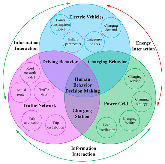
Figure 1.
Fusion architecture of ‘Electric vehicles–Power grid–Traffic network’.
3. Mining and Fusion of Online Ride-Hailing Trip Data
The ‘GAIA Open Dataset’ open source project by Didi Technology Co., Ltd., (No.2 Software Park, Haidian District, Beijing, China) Smart Transportation Platform provides raw trip data of online ride-hailing registered in the vast majority of Chinese cities. Fortunately, the open source database solves the problem that traffic operation data are not easy to obtain.
At present, various researchers [38,39,40,41] applied these data to model research for different fields. Compared with taxi trajectory data, Sui et al. [38] found that online ride-hailing has a lower empty-load rate and less detour behavior, which can provide better trip services. Wang et al. [39] analyzed residents’ hospitalization through this database, which contributed to the decision-making of infrastructure configuration for institutions, such as urban planning departments and hospitals. Sun et al. [41] analyzed spatio-temporal traffic line source emissions based on massive online car-hailing service data, which provided support for traffic network construction planning.
Herein, we continue to apply online ride-hailing trip data [37] into the study of urban EV fast-charging demand modeling. Because resident trip demand is the source of energy supply for vehicles, and traffic operation affects the spatio-temporal distribution of charging energy, it is worth noting that utilizing existing trip data to reasonably mine the required rules is the premise for constructing the charging demand prediction model.
The trip trajectory datasets we investigated were the same as the ones utilized in the previous charging demand prediction model [37]. Therefore, the subsequent data mining and fusion modeling in this section only explain the process and describe the analysis briefly. Reviewing reference [37] is encouraged if more details about the analysis process are sought. The analysis process of data mining and fusion is shown in Figure 2.
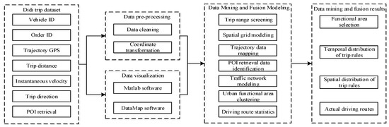
Figure 2.
Analysis process of data mining and fusion.
3.1. Data Description
Through applying from the official website, we obtained part of trip data sets in Nanjing, China, whose time spanned from 1 June 2016 to 31 June 2016. These data sets contain a total number of 31 data packets in days, with an average sampling interval of 3 s, and include 474,590 trip data chains. The main data formats and examples of trip data are shown in the Appendix A (Table A1 and Table A2).
As revealed by Table A1 and Table A2, the information that can be directly obtained includes time information of an order, trajectory GPS positioning point, dynamic travel information (distance, direction and speed of a trip) and Point of Interest (POI) information for functional area identification [42]. In addition, the POI retrieval data are encoded with five digits: the first two are the first-level category representing, respectively, residential areas, commercial areas, industrial areas, public service areas, road facility areas and green square areas from 01 to 06, and the last three are the second-level category representing the physical content of the functional area.
3.2. Data Pre-Processing and Visualization
Data pre-processing mainly included data cleaning and coordinate transformation. The main purpose of this step was to eliminate noise data and transform the GCJ-02 coordinate system of Didi trip GPS trajectory into the WSG-84 coordinate system for map drawing [30].
In data visualization the pre-processed data sets were visualized. We mainly used Matlab and DataMap for map drawing and data analysis [37].
Figure A1 and Figure A2 in the Appendix A are the daily trip statistics in June as well as the longitude and latitude coordinate distribution of trip order starting points and arrival points (OD data points), respectively.
3.3. Data Mining and Fusion Modeling
Visualization of the original trip data cannot reveal the resident’s trip rules and traffic operation characteristics. Therefore, it is necessary to conduct modeling analysis through data mining and fusion technology. The technical structure is shown in Figure 3.
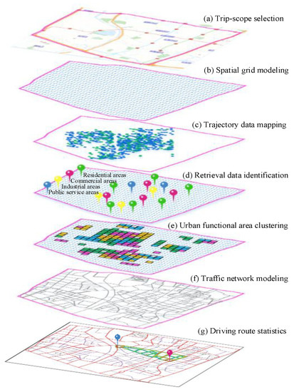
Figure 3.
Architecture of data mining and fusion.
As depicted in Figure 2, the brief steps of the architecture are outlined below.
3.3.1. Trip Range Screening
The trip range was between longitude (East) 118.7412–118.8249 and latitude (North) 32.0234–32.0633, the selected area was approximately 48.8 km2, and the circumference was approximately 27.9 km.
3.3.2. Spatial Grid Modeling
According to traffic planning theory, spatial grid modeling is used for centralized processing. In other words, the selected traffic plane was uniformly divided into different spatial grids as the research area depending on a spatial scale [37].
3.3.3. Trajectory Data Mapping
The trajectory data mainly contained temporal–spatial characteristics information for trips. Therefore, the cleaned data were mapped to the plane range area through coordinate transformation, and all trip data were represented as follows:
where indicates the trajectory data set for the jth order, , = 433,258, represents the longitude and latitude coordinates as well as the trip time stamp of departure point (O point), and represents the longitude and latitude coordinates as well as the trip time stamps of arrival point (D point), respectively.
Further, all the data of departure points and arrival points in the trajectory data set Ω were screened out to obtain the traffic OD matrix, which contains the position and time of starting and ending points as follows:
where represents the set of starting point (O point), and represents the set of ending point (D point).
3.3.4. POI Retrieval Data Identification
The POI retrieval data were used to identify and distinguish which specific functional area type the trajectory points belonged to [37].
3.3.5. Urban Functional Area Clustering
The adjacent grids with similar characteristics of trip demand and function area were clustered and merged by the time serial-based feature analysis method [34].
3.3.6. Traffic Network Modeling
Residents travel and vehicles drive on traffic networks, so the dynamic evolution process of traffic can be vividly depicted by traffic network modeling. Through the OpenStreetMap open source website (https://www.openstreetmap.org), we can obtain basic information of the regional road network in the selected trip range, and we can adopt the graph theory analysis method to describe the traffic network:
where G represents traffic network; V represents the set of all nodes in graph G, namely, the set of traffic nodes; E represents the set of all directed arcs in graph G, namely, the set of sections in traffic network; and W represents the set of road segment weights, namely, road impedance.
3.3.7. Driving Route Statistics
On the basis of traffic network modeling, all traffic segments between starting position and ending position of each order can be expressed as follows:
where represents the set of traffic nodes for the jth order travel trajectory, namely, driving route.
Then, all routes between starting and ending point (OD) can be counted:
where denotes the mth route between OD points, and indicates the mth route whose departure and arrival position of the jth order are consistent with OD points, namely direct driving routes between OD points. indicates the mth route whose departure and arrival position of the kth order includes OD points, namely indirect driving routes passing through OD points.
3.4. Data Mining and Fusion Results
3.4.1. Functional Area Selection
The traffic network model of third-grade roads and above in the selected area was built, and 14 commercial EV fast-charging stations in operation in the region were also analyzed to predict load demands. The structure topology of the traffic network and the distribution of fast-charging stations are shown in Figure 4, wherein geographical location information of each fast-charging station is shown in the Appendix A (Table A3). As depicted, there were 588 traffic nodes and 456 road segments in this area. The basic road planning data can be found on the OpenStreetMap website.
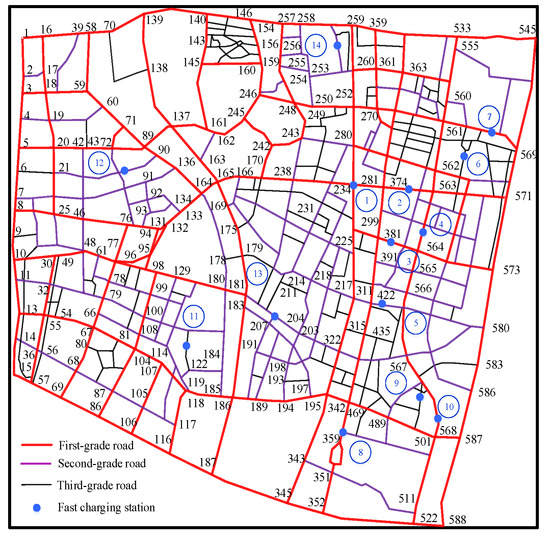
Figure 4.
Topological structure of traffic network and distribution of fast-charging stations.
3.4.2. Temporal Distribution of Trip Rules
We directly applied the data analysis and statistical results from [37], that is, the temporal distribution of departure time in the set and arrival time in the set had altered dates. Notably, the trip demand on weekdays was more than that on weekends and holidays. The traffic volume was mainly concentrated in the morning and evening peak hours, and that was significantly reduced at night.
3.4.3. Spatial Distribution of Trip Rules
Similarly, the spatial distribution of departure position in the set and arrival position in the set were different by region. As for weekdays, the high-density zones at starting and ending points of resident trips were residential areas and industrial areas. As for weekends and holidays, the zones with high-density at starting points were residential areas. However, the zones with high-density at ending points on weekends were industrial areas and public service areas, whereas that on holidays were commercial areas and public service areas.
3.4.4. Actual Driving Routes
Aiming at actual driving routes, route planning has the attributes of real-time dynamics and driver selection preference. Notably, they prefer to plan paths with the comprehensive goal of having the shortest time and distance.
4. Single Electric Vehicle Model
Through data modeling and mining, resident trip rules and traffic operation data are obtained. In this section, we build a single electric vehicle model to provide theoretical support for the charging load prediction framework.
4.1. Types and Quantities of EVs
In the previous study [37], according to ‘Implementation Plan for Promotion and Application of New Energy Vehicle in Nanjing during the 13th Five-Year Plan’ and the current development status of EVs in China, we introduced a total number of 23,780 vehicles, including private vehicles, taxis and other public vehicles. The specific number and attribute of each type of vehicle were consistent with the relevant description in [37], and readers may refer to this literature for more detailed information.
4.2. Driving Behavior Modeling
The OD matrix mined in Section 3.3 can vividly describe the temporal and spatial distribution of traffic trips. Therefore, we employed an OD analysis method to establish the dynamic and random driving behavior of vehicles.
- (1)
- Ev(i) is assigned departure time , departure position and destination position from OD sets and by Monte Carlo random sampling.where i represents the serial number of one EV, , .
- (2)
- The route with the most frequent usage between OD point is selected as the initial planned route for Ev(i).
- (3)
- When the charging requirement is not triggered, the initial planned route is the actual driving route . Otherwise, the triggering time and triggering location are recorded, and the destination location is changed to the recommended charging station location . k denotes the serial number of fast-charging stations, , . After completion of charging, the destination position is changed to , and the actual driving route is expressed as .where indicates the mark of vehicle charging requirement; when it is triggered , otherwise . indicates the moment when one vehicle arrives at a recommended fast-charging station, indicates the moment when one vehicle leaves a fast-charging station, and indicates the moment when one vehicle finally arrives at its destination.
- (4)
- Thus, each vehicle’s driving time consumption and distance on the entire traffic network are expressed as follows:where represents the road segment distance of actual driving route between position x and position y.
- (5)
- When Ev(i) arrives at its destination, the above steps are repeated to extract a new original departure and return matrix, and the simulation of tracking the vehicle trip trajectory is completed all in a day.
4.3. Charging Behavior Modeling
4.3.1. Battery Parameter Setting
According to the difference in battery capacity of each type of EV, this paper selects typical vehicles as simulation EV models. BAIC E150 was selected as the private vehicle, with a battery capacity of 25.6 and endurance mileage of 180 km; BYD E6 was selected as the taxi, with battery capacity of 60 and endurance mileage of 280 km; ZOYTE 5008ev was selected as the other public vehicles, with battery capacity of 32 and endurance mileage of 180 km.
In terms of the statistical results [18], we assumed that State of Charge (SOC) at the first trip time obeyed a normal distribution N (0.8, 0.1), so the initial battery capacity of each introduced vehicle can be generated combining with the battery capacity .
4.3.2. Power Consumption Per Unit Kilometer
Song et al. [43] discussed the relationship between EV consumption and traffic network under actual operating conditions, and they established a dynamic energy consumption model of EVs per unit kilometer in different grade traffic roads through microscopic driving characteristic parameter modeling, as follows:
where , and are the EV per unit kilometer consumption of the first-, second- and third-grade roads, respectively. represents the average velocity of road segment during time period T, which can be calculated by (13):
where represents the GPS instantaneous velocity of the rth vehicle trajectory passing through road segment during time period T.
4.3.3. Charging Requirement Judgment
According to the actual driving route and the dynamic energy consumption factor of each EV, the remaining battery capacity at time t is obtained:
where represents the decision variable of road segments. When one vehicle is driving on the traffic segment of actual route , , otherwise . is the length of traffic segment .
This paper mainly focuses on fast-charging load modeling for vehicles with urgent requirements on the road, so the charging requirement is generated depending on the driver’s mileage anxiety:
where denotes the range anxiety coefficient and has uniform distribution ~U[0.15,0.3] [13].
4.3.4. Fast-Charging Station Model
(1) Vehicle queuing model
The vehicle that needs charging has to go to the recommended fast-charging station for energy supply. The aggregated charging behavior conforms to First Come First Service Theory [44]. Each vehicle receives charging service via waiting in a queue. Therefore, the specific steps of the queuing model are as follows:
(1) The average arrival rate of each vehicle that needs charging and the average service rate of each charging pile for fast-charging station k are counted:
where , respectively represent the number of vehicles arriving at fast-charging station k at time t and the number of vehicles for charging service at a single charging pile;
(2) According to the recurrence formula [44], the idle probability of one charging pile and the average queue length of vehicles at time t for fast-charging station k can be obtained as follows:
where n indicates the number of vehicles served by all charging piles, and represents the number of charging piles equipped in fast-charging station k. In our study, each fast-charging station was equipped with 30 charging piles. Let indicate the utilization rate of charging facilities in fast-charging station k: .
(2) Vehicle waiting duration
When the number of vehicles that need charging exceeds the number of charging piles, the vehicles need to wait in line, so the average charging waiting duration of fast-charging station k is as follows:
Each vehicle’s charging waiting duration is determined by
where represents the number of vehicles at the station when Ev(i) arrives at fast-charging station k, including vehicles being recharged and waiting for recharging, which can be obtained from the following equation:
where represents the number of vehicles at fast-charging station k at the initial moment. represents the serial number of charging piles, . represents the number of leaving vehicles that have been recharged by the th charging pile at fast-charging station k during the time period from to .
(3) Vehicle charging duration
When EV users receive charging services at a fast charging station, considering the factors such as charging duration and charging cost, they would not fully but partially charge the battery. Thus, denotes the finishing SOC value which obeys a normal distribution N (0.85, 0.3), and the charging duration is defined as:
where denotes the charging efficiency, and the value range is 0.8~0.9; denotes the battery capacity of a vehicle arriving at fast-charging station k; denotes the charging power of charging pile . In terms of QC/T 841-2010 ‘Electric Vehicle Conductive Charging Interface’, is set as 70 kW (Level 3).
(4) Vehicle charging cost
Finally, the user pays cost to charging service providers depending on the price in different periods:
where represents the time-of-use price of charging service: 2 yuan/() for peak periods (8:00–12:00, 14:30–21:00 and 17:00–21:00), 1.5 yuan/() for flat hump periods (12:00–14:30 and 21:00–24:00) and 0.5 yuan/() for off-peak periods (00:00–08:00).
5. Human Behavior Decision-Making Model
In real life, human beings’ decision-making and judgment of driving and charging behaviors are limited to their subjective psychological factors and non-comprehensive cognitive level. Thus, they do not always select the scheme with the overall maximum utility and optimal individual interest.
From the perspective of human behavior, this section introduces Regret Theory [45,46] to recommend fast-charging stations for vehicles that need charging.
5.1. Basic Principle of Regret Theory
Regret Theory, based on the regret avoidance psychology of human behavior in discrete event selection [47], describes the utility brought by decision-makers to focus on both the selected scheme and alternative scheme when making a choice. When the utility of the selected scheme is better than the others, it will produce an enjoyable experience for decision-makers. Otherwise, it will leave them with a regret experience. Such a human emotional state can be quantified by a regret function, which is
where represents the random regret value of the selected scheme . represents the determined regret value generated by the choice of scheme , which reflects the decision-maker’s perception of the scheme. represents the estimated parameter of attribute a, which reflects the decision-maker’s preference for attribute a. and represent the attribute values of scheme i and scheme j, respectively. represents the random regret error of scheme i, which obeys independent and identical distribution. represents the probability of the chosen scheme .
Figure 5 shows the decision-making and selection process of Regret Theory. Combined with Figure 5 and Equation (25), the essence of the theory’s decision-making rule is as follows: When the alternative scheme set has multiple schemes for selection, the utility difference between each scheme of attribute values is weighed repeatedly. If remains in the intermediate state, the regret value of the final selected scheme is at a minimum and the probability of the scheme is at a maximum. That is, decision-makers tend to compromise. It is obvious that the regret avoidance psychological choice behavior is more consistent with the real thinking habits of human beings.
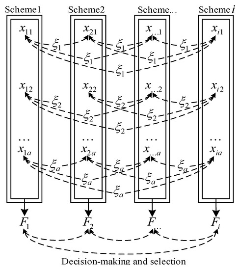
Figure 5.
Decision-making and selection process of Regret Theory.
5.2. Fast-Charging Station Recommended Model
Regret Theory provides an effective research tool for the analysis of human choice behavior. Based on this theory, we established a recommendation model for fast-charging stations. All time consumption T and charging cost I are taken as attribute values, and the scheme set is each fast-charging station. The specific model is as follows:
where denotes the specific scheme of the selected fast-charging station. That is, considering the effect of total time consumption T and charging cost I, when is the smallest, the suitable fast-charging station is recommended to each user.
Finally, the fast-charging demand load for the selected area is determined by
where represents the number of EVs in fast-charging station k at time t. represents the charging status marker of the ith EV recommended to fast-charging station k. When a vehicle is recharged, the marker is designated as 1; otherwise, it is designated as 0.
6. Electric Vehicle Fast-Charging Demand Forecasting Model
The framework of electric vehicle fast-charging demand prediction model is shown in Figure 6.
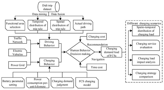
Figure 6.
Framework of electric vehicle fast-charging demand prediction model.
- (1)
- Mine and fuse Didi order data to obtain the characteristics and rules needed for residents’ trip demands;
- (2)
- Use the above statistical rules and regenerative data as the basis for the EV driving behavior model, and establish a single EV charging behavior model;
- (3)
- Consider a behavior decision model with time consumption and charging cost to plan the route and recommend the fast-charging station for EV owners;
- (4)
- Calculate the charging demand of the fast-charging station and evaluate the charging load operating characteristics in different scenarios.
7. Path Planning Experiments
The EV owner needs path planning and guidance whether they are driving normally or charging emergently. Therefore, this section designs the path planning experiments and carries out the trip simulation for 23,780 electric vehicles (including 11,890 private vehicles, 4756 taxis and other public vehicles) introduced in this area.
First of all, we chose three typical traffic scenarios, namely the peak time period of traffic trips (07:00–08:00), the flat hump time period of traffic trips (15:00–16:00) and the off-peak time period of traffic trips (02:00–03:00). The actual driving routes of six pairs of traffic starting and ending nodes in three time periods are shown in Figure 7. In addition, in order to compare with Actual Path (AP), we also selected the Shortest Length Path (SLP) and Shortest Time Path (STP) Dijkstra methods to search road segment weight W [37]. From 07:00 to 08:00, the specific search path with the traffic starting point 169 and traffic ending point 566 searched by the above three path methods is shown in Figure 8.
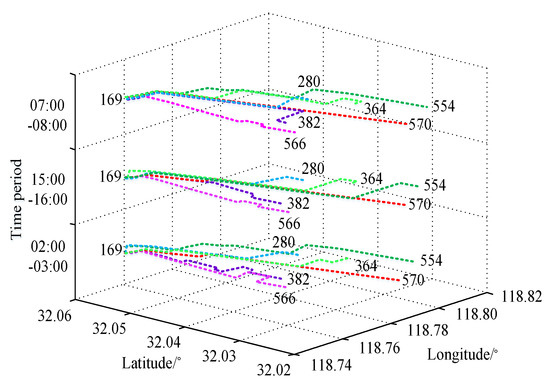
Figure 7.
Actual route under peak, flat hump and off-peak time periods.
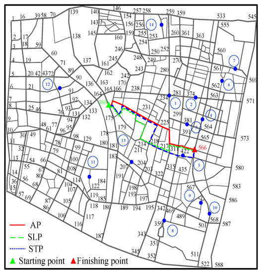
Figure 8.
Comparison of routes searched by Actual Path, Shortest Length Path and Shortest Time Path STP.
It can be seen from Figure 7 and Figure 8 that, intuitively, the actual path had real-time dynamic characteristics in traffic path planning, even if the same OD nodes passing through road segments were not completely consistent in different time periods. Similarly, the path searched by Dijkstra target path optimization method did not completely coincide with the actual path. That is, the actual path was a compromise between time consumption and distance.
Next, in order to quantitatively analyze the search effect of different path methods, Figure 9 shows the average coincidence rates of all OD node paths searched by SLP, STP and AP methods in different time periods. The traffic operation indexes of the three methods are shown in the Appendix A (Table A4).
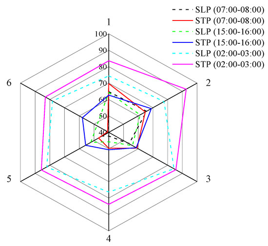
Figure 9.
Comparison of path coincidence rates of each path method under peak, flat hump and off-peak time periods.
As depicted by Figure 9 and Table A4, the coincidence rates of STP, SLP versus AP during 02:00–03:00 were the highest, which were 84.55% and 80.18%, respectively, followed by 15:00–16:00, where the coincidence rates were respectively 64.14% and 54.28%. The lowest was during 07:00–08:00, with coincidence rates of 64.14% and 54.28%, respectively. It shows that the lower the traffic volume is, the closer the path planned by the Dijkstra target path optimization method is to the actual path. In addition, the SLP method takes the shortest distance as its search target, which is a static path planning method. The search result of road segments is fixed routes, which is not affected by time fluctuations. Therefore, SLP method’s average mileage and proportion of the first, second and third road grades were constant in the above three time periods. Whereas, STP and AP methods are dynamic path planning methods, and the traffic operation indexes in each time period are variable. Compared with the static path planning method, the two dynamic path planning methods required more iterative steps and real-time information to search for road segments, so their running times were much longer than that of the static path method. The average running times of AP, STP and SLP in the three periods were 18.22, 13.87 and 5.30 s, respectively. However, the AP method based on decision-making behavior involves many model factors, and the running time of each period was the longest, so the computational performance can be further improved.
For the average mileage index, the SLP method with the shortest path objective optimization had the least mileage, which was 7.23 km. However, STP method sacrificed a certain benefit of mileage to maximize the benefit of time consumption, and its average mileage from 07:00 to 08:00 was the highest, reaching 10.89 km.
For the average time consumption index, on the contrary, in order to save the driving mileage, SLP method lacked considering the benefit of time consumption. During 07:00–08:00, the average time consumption was the longest, which was 35.77 min, whereas the shortest average time consumption was 14.89 min from 02:00 to 03:00, which was obtained by the STP method. As mentioned before, the search results of the AP method in each time period were approximate to the middle value for the above two indexes.
For the proportion of all road grade indexes, the higher the grade of road is, the larger the traffic proportion is. The proportion of the first road grade was the highest, and the results planned by all route methods exceeded 36%. It indicates that each method tends to choose high-grade roads to drive in different time periods. However, STP has a higher proportion of the third road grade than SLP and AP method, and the proportion in each time period exceeded 28%. It also explains that STP method may save time by taking a short cut on low-grade roads so as to maximize the time benefit.
8. Case Studies and Analysis
After the data mining and path planning experiments, for the sake of verifying the implementation effect of EV fast-charging demand forecasting model, this section conducts five groups of charging experiments in different scenarios and analyzes actual charging load operation characteristics. The input–output data and used models in each case study are shown in the Appendix A (Table A5).
8.1. Temporal–Spatial Distribution of Fast-Charging Demand Load
Firstly, with the time interval of one hour, the temporal distribution of the average number of vehicles required for recharging in each fast-charging station on weekdays was created. Time consumption estimation parameter and charging cost estimation parameter in the recommended fast-charging station model were uniformly designated as 1. That is, we assumed the decision-maker had the same degree of preference for both attributes, and the result is shown in Figure 10.
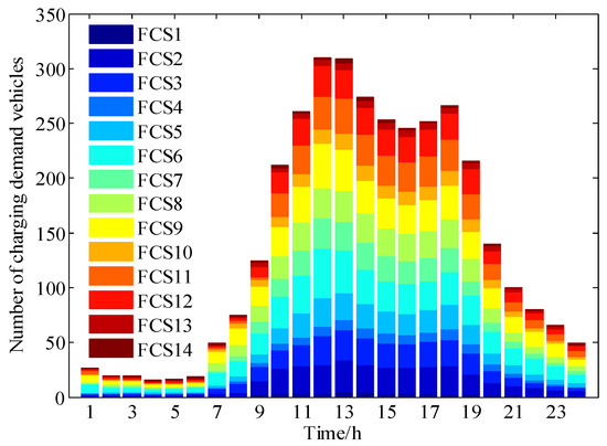
Figure 10.
Temporal distribution of vehicles with fast-charging requirements.
As depicted, as a whole, due to the impact of traffic flows on weekdays, the temporal distribution of the average number of fast-charging vehicles was uneven. The peak periods of charging demand were from 12:00 to 13:00 at noon, reaching 321.23 vehicles, and from 17:00 to 18:00 in the evening, reaching 265.32 vehicles. The station serving the largest number of vehicles was FCS1 because it is located in the central zone of the city, with the largest number of guiding vehicles for recharging, reaching 23.15 vehicles. Conversely, FCS12 is located at the edge of the city, and the number of served vehicles was the least, only 12.23 vehicles.
Hereafter, Figure 11 shows the spatial distribution of vehicle charging demand during the peak hour (12:00–13:00). As depicted, the fast-charging demand was during emergencies. The trigger position of vehicle charging requirements was mainly concentrated on the road, but the distribution in the urban center zone was more than that in the marginal zone. Moreover, the hot spots of charging demands were distributed in the following road segments: 234–281, 270–374, 311–315 and 469–489. The charging demand of the above road segments was more than 30 vehicles, which mainly belonged to commercial areas according to POI retrieval.
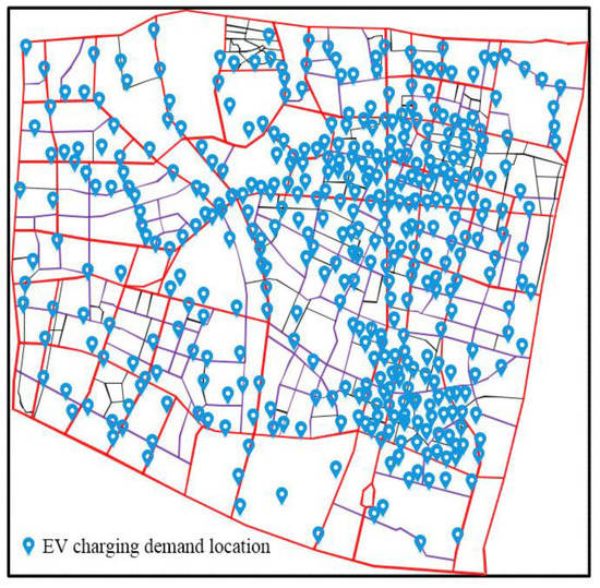
Figure 11.
Spatial distribution of vehicles with fast-charging requirements in the peak period.
We also calculated the average charging demand load distribution of each fast-charging station on weekdays, weekends and holidays, with the 15 min simulation step. The results and indexes of load distribution characteristics of different date types are shown in Figure 12 and Table 1.
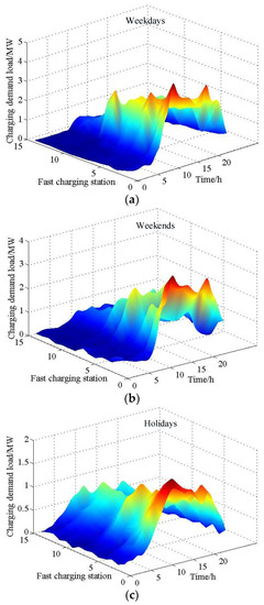
Figure 12.
Charging demand load of each fast station on weekdays, weekends and holidays. (a) Charging demand load on weekdays. (b) Charging demand load on weekends. (c) Charging demand load on holidays.

Table 1.
Load distribution characteristics of different date types.
As revealed by Figure 12 and Table 1, since the resident trip demand was mainly concentrated in the daytime, the charging demand load in this time period was greater than that in the evening, and the peak–valley difference in each fast-charging station fluctuated greatly. It was found that the running time of weekday loads was longer than that of weekends and holidays.
On weekdays, the largest fast-charging station with average charging demand load was FCS1, which reached the peak load at 11:45 with 1.56 MW, the valley load appeared at 02:15 with 0.14 MW, and the peak–valley difference was 1.42 MW. The lowest was FCS11, which reached the load peak 0.96 MW at 12:15, the valley load appeared at 02:30, only with 0.07 MW, and the peak–valley difference dropped to 0.89 MW.
On weekends, compared with weekdays, the average charging demand load decreased significantly. The station with the largest load demand was still FCS1, with peak and valley loads of 1.42 and 0.06 MW respectively, and the peak–valley difference was 1.36 MW. The station with the lowest load demand was FCS12, whose peak and valley loads were 0.93 and 0.06 MW respectively, and the peak–valley difference was 0.87 MW.
On holidays, the traffic trip volume of this date type was significantly lower than that of weekdays and weekends, so the overall charging demand load level was relatively low. The charging station with the largest load demand was FCS2, and the peak load reached 1.23 MW. The charging station with the lowest load demand was FCS13, whose valley load was only 0.07 MW.
What is more, we divided and sorted the fast-charging stations according to the type of functional areas, and the thermal distribution of charging demand loads in each functional area is shown in Figure 13.
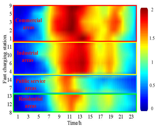
Figure 13.
Charging demand load of fast-charging stations in each functional area.
From Figure 13, from the aspect of spatial distribution for charging demands, the fast-charging stations in commercial and industrial areas were mostly concentrated in densely populated urban center zones, with a high popularity of charging facilities and dense traffic flows. It is worth noting that the fast-charging demand load in the above two areas was much higher than that in public service areas and residential areas, accounting for 73.23% of the total charging load.
From the aspect of temporal distribution for charging demands, influenced by residents’ trip rules, those in commercial and industrial areas were mainly concentrated in the period from 08:00 to 18:00. Those in public service areas and residential areas were mainly distributed between 09:00 and 12:00. In addition, due to the return trip behavior of residents, there were also hot spots of charging demands in residential areas between 18:00 and 19:00.
8.2. Fast-Charging Demand Load with Different Path Strategies
Secondly, in Section 7, it was found that vehicle driving and navigation routes obtained by each path planning strategy were quite different. Therefore, in order to compare with our strategy, this section designs the charging demand load test for AP, SLP and STP strategies. As regards the SLP strategy, that is, when the vehicle is driven normally, the shortest distance is the goal for planning. When the fast-charging requirement is triggered, the fast-charging station with the shortest charging distance is navigated for recharging, without considering the constraints of charging cost and duration. Similarly, as regards the STP strategy, the path search target of normal driving and emergency charging is changed to that with the shortest time.
Vehicle driving planning and charging navigation simulations were carried out according to the above-mentioned path strategies. On weekdays, SOC statistics of vehicles arriving at a typical fast-charging station, FCS1, all day performed by each path strategy is shown in Figure 14, and the average charging demand load distribution of all fast-charging stations is shown in Figure 15.
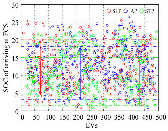
Figure 14.
SOC of vehicles arriving at fast-charging station.
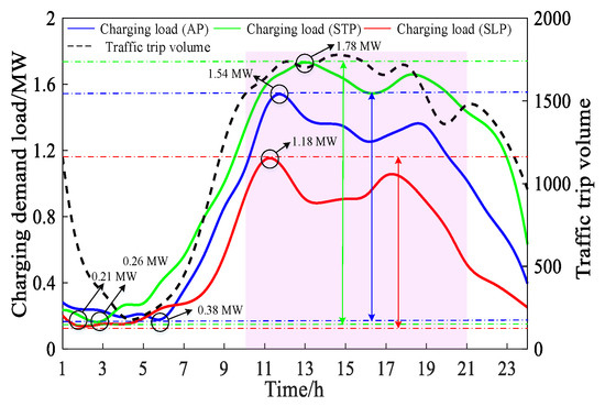
Figure 15.
Comparison of charging demand load among AP, SLP and STP path strategies.
As revealed by Figure 14 and Figure 15, the STP strategy planned paths with the shortest time. In the process of driving and charging route search, there was a certain detour phenomenon in order to maximize the time utility, which increased the energy consumption of vehicle driving. Its SOC ranged from 2.7% to 15.0%, with an average of 7.76%. In contrast, the SLP strategy took the shortest driving distance as the planning goal, and the overall vehicle mileage was less, which ranged between 4.9% and 20.0%, and the average SOC was 12.45%. Moreover, the SOC distribution range of the AP strategy was concentrated between 4.1% and 17.8%, and the average SOC was 10.25%.
Accordingly, the STP strategy had the largest charging load, followed by the AP strategy, whereas overall driving and charging mileage in SLP were less than the other two strategies, with the least overall charging load. The average charging loads of STP, AP and SLP in the whole day were 1.38, 1.16 and 0.87 MW respectively. The peak charging load was mainly concentrated in the period from 11:00 to 13:00, which overlapped with the peak period of traffic trips.
In addition, during 10:00–21:00, the traffic flow fluctuated greatly. In this period, the charging load in the whole day accounted for a relatively high proportion. STP, AP and SLP strategies accounted for 66.58%, 60.23% and 70.56%, respectively, whereas their peak valley differences were 1.05, 0.78 and 0.87 MW respectively. In addition, in other time periods, with the decrease of traffic trip flow, the charging demand load decreased and peak valley differences of loads reduced to 0.87, 0.69 and 0.65 MW respectively.
Further, for the sake of evaluating the charging service efficiency of the three path strategies, the duration of vehicles entering the station (namely, the sum of charging waiting duration and fast-charging duration ) and charging cost were selected as evaluation indexes. The statistical results of the number of vehicles required for recharging in each time interval are shown in Figure 16. The evaluation indexes of charging station navigation for each route strategy are shown in Table 2.
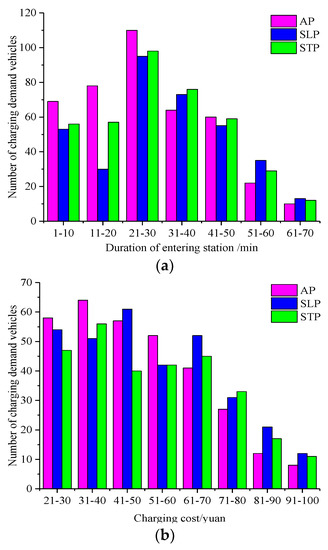
Figure 16.
Duration of entering station and charging cost for AP, SLP and STP path strategies. (a) Duration of entering station for AP, SLP and STP path strategies. (b) Charging cost for AP, SLP and STP path strategies.
Table 2.
Evaluation indexes of charging station navigation for each route strategy.
From Figure 16 and Table 2, SLP and STP strategies selected nearby charging based on the optimal distance and travel time consumption, which were a disorderly charging recommendation strategy. However, the AP strategy restricted charging guidance through the Regret Model, which had an orderly charging recommendation strategy. The average charging durations of AP, SLP and STP strategies were 21.37, 24.87 and 29.78 min, and the average charging costs were 45.23, 41.28 and 51.23 yuan. Although there was a certain phenomenon of vehicle queuing in all three strategies, compared with the disordered recommendation strategy, the orderly charging method shortened the waiting time.
For the entering station duration index, although the time interval with the most vehicles entering station of all the three strategies was 21–30 min, but the proportions of AP, SLP and STP strategies with durations of more than 30 min were 32.35%, 42.95% and 44.56%, respectively.
For the charging cost index, the maximum charging cost ranges of both AP and STP strategies were 31–40 yuan, whereas that of the SLP strategy was 41–50 yuan. However, the charging costs of AP, SLP and STP strategies over 60 yuan accounted for 33.58%, 37.89% and 34.12%, respectively.
It can be seen from the above analysis that our AP path guidance strategy adopted an eclectic recommended fast-charging station approach. Although, there is no guarantee that duration and charging cost of each individual EV will be maximized. However, the eclectic selection of fast-charging stations from the alternatives reduced the proportion of vehicles in the maximum range of service indicators, which tended to balance vehicle service indicators.
8.3. Fast-Charging Demand Load with Different Charging Modes
As one of the important factors affecting fast-charging demand loads, the charging mode in this paper was set as the random charging mode shown in Equation (23). Therefore, different charging models were exploited to study the charging load operation characteristics of FCS1, and the results are shown in Figure 17. Wherein, ‘100% full-charged’ stands for charging mode 1 (M1), indicating that all vehicles arriving at a station choose the battery full state. ‘100% random-charged’ stands for charging mode (M2), indicating that all arriving vehicles choose random charging mode. ‘60% random-charged, 40% full-charged’ stands for charging mode 3 (M3), indicating that 60% of arriving vehicles choose the random charging mode, and 40% of them choose the battery full state. ‘70% random-charged, 30% full-charged’ stands for charging mode 4 (M4). ‘80% random-charged, 20% full-charged’ stands for charging mode 5 (M5).
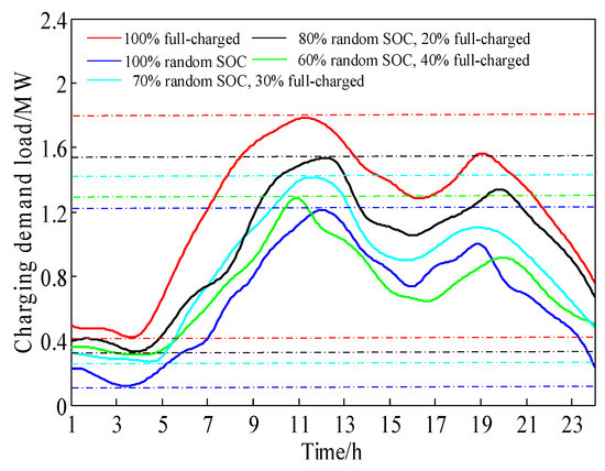
Figure 17.
Charging demand load for different charging modes.
Table 3 shows the specific values of service indexes for different charging modes. Combined with Figure 17 and Table 1, it can be seen that charging mode 1 had the largest charging demand, and the peak load reached 1.87 MW, whereas charging mode 2 had the lowest charging demand, and the peak load was only 1.26 MW. As the proportion of vehicles with full battery state increased, the charging demand load also grew. When the proportion of vehicles choosing battery full-charged mode increased by each 1%, the charging demand load grew by 5.36 kW. Additionally, charging mode 1 acquired the maximum value among all service indexes. It indicates that when the owner tends to choose the battery full state, the charging duration and the charging cost are increased, so that the vehicle’s waiting duration and charging demand also increase. Therefore, the random charging mode is more consistent with the actual charging situation of owners, and it is easier to obtain high-quality charging services.
Table 3.
Comparison of service indicators of different charging modes.
8.4. Fast-Charging Demand Load with Different Charging Facility Ratios
Moreover, the power configuration of charging facilities is another important factor affecting charging demand loads. Therefore, the same analysis method [34] was adopted to introduce Charging Facility Ratio (CFR). That is, the ratio of the number of charging piles in fast-charging stations to the peak number of vehicles with charging requirements.
In this paper, the charging pile powers were respectively 70 kW (CFR-70) and 120 kW (CFR-120) for analysis. Under different CFR conditions, the peak load distribution of all fast-charging demands in the selected area is shown in Figure 18.
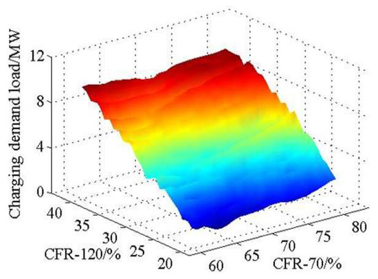
Figure 18.
Charging load peak under different Charging Facility Ratio conditions.
Figure 19 shows the typical charging demand load when CFR-120 was under 20%, 25%, 30% and 35%, respectively. Meanwhile, Figure 20 shows their corresponding duration of entering at a station.
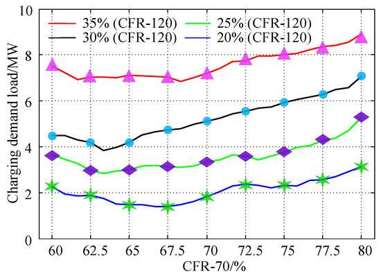
Figure 19.
Charging load peak under different groups of Charging Facility Ratio.
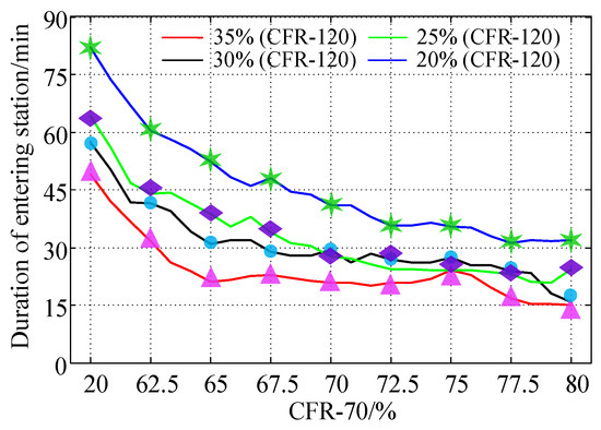
Figure 20.
Duration of entering station under different groups of CFR.
As depicted from Figure 18 to Figure 20, on the whole, when CFR with different charging powers increased, the charging demand load grew to some extent. For each 1% increase in CFR-70, the charging demand load grew by 0.12 MW, whereas for each 1% increase in CFR-120, the charging demand load grew by 0.19 MW. Moreover, when the charging powers of CFR-70 and CFR-120 increased by each 1%, the corresponding duration of entering a station reduced by 3.47 and 4.27 min, respectively. It indicates that charging facilities with high power have a greater impact on charging demand than that with low power; the higher the power of charging facilities is, the greater the reduction duration of entering a station will be.
8.5. Utility Evaluation of Human Behavior Decision-Making Model
At last, in the experimental analysis mentioned above, estimated parameters and , respectively belonging to time consumption and charging cost, are both fixed as 1. For the sake of evaluating the influence of the two estimated parameters on the human behavior decision-making model, we discuss the effect of a typical fast-charging station, FCS1, with different estimated parameters on time consumption and charging cost. The average of all vehicles recharged in this station on weekdays was taken as the evaluation index, and the results are shown in Figure 21.
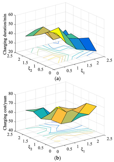
Figure 21.
Charging duration and charging cost with different estimation parameters. (a) Charging duration with different estimation parameters. (b) Charging cost with different estimation parameters.
Moreover, Table 4 lists the specific results of evaluation indexes of different groups of estimated parameters. Combined with Figure 20 and Table 4, it can be seen that, as a whole, with the improvement of estimated parameters, the attribute weights of charging duration and charging cost increased. In that case, the regret of decision-makers eventually increased, and the charging frequency of FCS1 decreased, which reduced charging duration and charging cost. Furthermore, the influence of estimated parameter on charging duration was larger than that of estimated parameter on charging cost. For each 1 increase of , the average charging duration reduced by 9.76 min, whereas for each 1 increase of , the average charging cost reduced by 7.87 yuan. It indicates that the decision maker’s sensitive experience to charging duration was greater than that to the charging cost. Specially, when , , the minimum charging duration and charging cost are obtained, with 37.8 min and 45.8 yuan respectively. In addition, the charging load demand was determined together by the two estimation parameters, so there was no obvious fluctuation rule.
Table 4.
Evaluating indicators under different groups of estimation parameters.
9. Conclusions
This paper proposes an urban EV fast-charging demand forecasting model to plan driving paths and recommend fast-charging stations, via mining of Didi trip data and modeling of single EV, along with using a human decision-making model. The effectiveness of the proposed method is verified by the path planning experiment and different charging demand load scenarios, and the most important results and main contributions of the proposed model are as follows.
Through the mining and fusion of Didi ride-hailing trip orders, the regenerative characteristic data needed for vehicle travel can be obtained, which solves the difficulty in traffic data acquisition. According to each date type and functional area, the residents’ trip rules are obviously different, and the traffic volume on weekdays is larger than that on weekends and holidays. In addition, the actual driving route has real-time fluctuations, and the driver tends to choose high-grade traffic roads.
The residents’ traffic trip rule affects the urban fast-charging demand. The larger the traffic travel volume is, the higher the EV charging demand load will be. When the vehicle charging mode is selected as the battery full state, compared with the random charging mode, it increases the fast-charging demand load and reduces the charging service quality. The higher the charging facility power is, the greater the charging demand loads will be.
By selecting and comparing the alternatives, the human behavior decision-making model adopts a compromise approach to carry out path planning and charging guidance for vehicles with fast-charging requirements. The recommendation method of the compromise strategy is more consistent with human behavior decision psychology and the actual running state of charging loads. Moreover, compared with the charging cost attribute, the user has a higher regretful experience for the charging duration attribute.
Nevertheless, it is noteworthy that we only employed the actual data from the traffic side for data mining. In the next work, the whole data-chain including distribution network, environment and charging station might be further modeled and analyzed. Also, the discussion on the optimal running state of performance parameters for the human behavior decision-making model will be continued. In addition, this paper only analyzes the charging demand load modeling under the operation mode of grid to vehicle (namely, G2V). Based on the established behavior decision-making model, we can continue to investigate the discharge demand load model under the operation mode of vehicle to grid (namely, V2G), and we can formulate an orderly charging control strategy to evaluate the impact of the aggregate charging and discharging behavior on distribution network planning and transportation network operation.
Author Contributions
Data curation, X.X., T.Z. and H.W.; Formal analysis, Q.X.; Investigation, Q.X. and Z.C.; Methodology, Q.X. and Z.Z.; Project administration, Z.C.; Supervision, X.H. All authors have read and agreed to the published version of the manuscript.
Funding
This research was supported by The Major State Research Development Program of China (2016YFB0101800), and State Grid Anhui Science and Technology Project (SGAHHF00FZJS 1901246).
Acknowledgments
The authors gratefully acknowledge GAIA Open Dataset for access to the data on which the paper was based.
Conflicts of Interest
The authors declare no conflict of interest.
Abbreviations/Nomenclature
| EV | Electric vehicle |
| FCS | Fast-charging station |
| OD | Origin Destination |
| POI | Point of Interest |
| AP | Actual path |
| SLP | Shortest length path |
| STP | Shortest time path |
| Sets | |
| Trajectory data set for the jth order | |
| Set of starting point | |
| Set of ending point | |
| V | Set of traffic nodes |
| E | Set of sections in a traffic network |
| W | Set of road segment weights |
| Set of traffic nodes for the jth order trip trajectory | |
| The mth route between OD point | |
| Initial planned route | |
| Actual driving route | |
| Parameters | |
| G | Traffic network |
| Charging station location | |
| Mark of charging requirement | |
| Driving distance | |
| Road segment distance | |
| Battery capacity | |
| Initial battery capacity | |
| Remaining battery capacity at time t | |
| Range anxiety coefficient | |
| Number of charging piles | |
| Utilization rate of charging facilities | |
| Charging efficiency | |
| Charging power of charging pile | |
| Time-of-use price of charging services | |
| Estimated parameter | |
| Attribute values | |
| Variables | |
| Latitude and longitude coordinates of departure point | |
| Latitude and longitude coordinates of arrival point | |
| Starting time | |
| Arriving time | |
| Triggering time of charging requirement | |
| Triggering location of charging requirement | |
| Destination location | |
| Moment arriving at the FCS | |
| Moment leaving the FCS | |
| Moment arriving at the destination | |
| Driving time consumption | |
| EV per-unit kilometer power consumption in different grades traffic roads | |
| Average velocity | |
| Decision variable of road sections | |
| Average arrival rate | |
| Average service rate | |
| Idle probability of one charging pile | |
| Average queue length | |
| Average charging waiting duration | |
| Charging waiting duration | |
| Number of vehicles at station | |
| Serial number of charging piles | |
| Charging duration | |
| Finishing charging SOC value | |
| Battery capacity of a vehicle arriving at FCS | |
| Charging cost | |
| Random regret value | |
| Determined regret value | |
| Random regret error | |
| Probability of chosen scheme | |
| Fast-charging demand load | |
Appendix A
Table A1.
Description of Didi trip data format.
Table A1.
Description of Didi trip data format.
| Field Name | Field Type | Field Description |
|---|---|---|
| Vehicle ID | Varchar | Anonymized |
| Order ID | Varchar | Anonymized |
| GPS instantaneous time | Datatime | Format yyyy/mm/dd hh: mm: ss |
| Trajectory GPS longitude | Double | Format dd.dddd, GCJ-02 coordinate system |
| Trajectory GPS latitude | Double | Format dd.dddd, GCJ-02 coordinate system |
| Trip distance | Double | Format dd.dddd, Unit km |
| Instantaneous velocity | Double | Format dd.dddd, Unit km/h |
| Trip direction | Double | Format dd.dddd, Unit degree |
| POI retrieval | Varchar | Format dd.dddd, Digitally encoded |
Table A2.
Example of Didi trip data.
Table A2.
Example of Didi trip data.
| Vehicle ID | Order ID | GPS Instantaneous Time | Trajectory GPS Longitude/° | Trajectory GPS Latitude/° | Instantaneous Velocity/km/h | Trip Distance/km | Trip Direction/° | POI Retrieval |
|---|---|---|---|---|---|---|---|---|
| 19b74075cf71 | 75cf0ae50ee63 | 2016/6/1 18:27:00 | 118.7753 | 32.0486 | 21.2345 | 2.1256 | 11.3651 | 01.001 |
| 19b74075cf71 | 75cf0ae50ee63 | 2016/6/1 18:27:03 | 118.7756 | 32.0487 | 22.4458 | 2.1432 | 5.6742 | 01.001 |
| 19b74075cf71 | 75cf0ae50ee63 | 2016/6/1 18:27:06 | 118.7757 | 32.0487 | 25.6789 | 2.1639 | 5.9264 | 01.001 |
| 19b74075cf71 | 75cf0ae50ee63 | 2016/6/1 18:27:09 | 118.7772 | 32.0486 | 29.6698 | 2.1853 | 6.1024 | 01.001 |
| 19b74075cf71 | 75cf0ae50ee63 | 2016/6/1 18:27:12 | 118.7799 | 32.0485 | 34.2359 | 2.2100 | 6.2314 | 01.002 |
| 19b74075cf71 | 75cf0ae50ee63 | 2016/6/1 18:27:15 | 118.7839 | 32.0484 | 34.2489 | 2.2385 | 5.9987 | 01.002 |
| … | … | … | … | … | … | … | … | … |

Figure A1.
Display of the quantity of Didi online car-hailing trips in June.

Figure A2.
Distribution of starting and arriving points. (a) Distribution of origin points. (b) Distribution of destination points.
Table A3.
Geographic position information of fast-charging stations.
Table A3.
Geographic position information of fast-charging stations.
| FCS Number | Latitude/° | Longitude/° | Road Location | Functional Area |
|---|---|---|---|---|
| 1 | 32.0451 | 118.7894 | 234–281 | commercial area |
| 2 | 32.0497 | 118.7910 | 374–375 | commercial area |
| 3 | 32.0411 | 118.7938 | 391–565 | commercial area |
| 4 | 32.1034 | 118.9164 | 478–481 | industrial area |
| 5 | 32.0383 | 118.7962 | 433–567 | commercial area |
| 6 | 32.0526 | 118.8026 | 561–562 | industrial area |
| 7 | 32.0504 | 118.7984 | 568–569 | public service area |
| 8 | 32.0262 | 118.7990 | 342–359 | residential area |
| 9 | 32.0262 | 118.7990 | 490–492 | commercial area |
| 10 | 32.0195 | 118.7968 | 493–568 | industrial area |
| 11 | 32.0265 | 118.7500 | 120–122 | industrial area |
| 12 | 32.0448 | 118.7529 | 73–90 | residential area |
| 13 | 32.0247 | 118.7571 | 179–200 | residential area |
| 14 | 32.0646 | 118.7971 | 252–259 | public service area |
Table A4.
Comparison of traffic operation index of each path method under peak, flat hump and off-peak time periods.
Table A4.
Comparison of traffic operation index of each path method under peak, flat hump and off-peak time periods.
| Time Period | Path Method | Average Mileage/km | Average Time Consumption/min | Proportions of the First, Second and Third Road Grade/% | Running Time/s |
|---|---|---|---|---|---|
| 07:00–08:00 | AP | 9.66 | 25.15 | 44.33/28.79/26.88 | 24.22 |
| SLP | 7.23 | 35.77 | 48.56/24.55/26.89 | 5.23 | |
| STP | 10.89 | 19.12 | 40.95/28.77/30.28 | 19.27 | |
| 15:00–16:00 | AP | 8.63 | 20.43 | 40.22/34.42/25.36 | 17.26 |
| SLP | 7.23 | 18.55 | 48.56/24.55/26.89 | 5.67 | |
| STP | 9.56 | 15.56 | 36.89/32.66/30.45 | 12.22 | |
| 02:00–03:00 | AP | 7.83 | 15.56 | 45.23/31.12/23.65 | 13.19 |
| SLP | 7.23 | 21.78 | 48.56/24.55/26.89 | 4.99 | |
| STP | 8.15 | 14.89 | 43.22/28.55/28.23 | 10.12 |
Table A5.
Input–output data and used models in each case study.
Table A5.
Input–output data and used models in each case study.
| Input Data | Input Models | Output Results | |
|---|---|---|---|
| Case Study 1 | 1. Trip data on weekdays, weekends and holidays 2. Geographic position information of FCSs | 1. Single electric vehicle model 2. Human behavior decision-making model | Temporal–spatial distribution of fast charging demand load |
| Case Study 2 | 1. Trip data on weekdays 2. Geographic position information of FCSs 3. Charging price of FCSs | 1. Single electric vehicle model 2. Human behavior decision-making model 3. STP, SLP methods | Fast charging demand load with different path strategies |
| Case Study 3 | 1. Trip data on weekdays 2. Geographic position information of FCS1 3. Charging price of FCS1 | 1. Single electric vehicle model 2. Human behavior decision-making model 3. Different charging modes | Fast charging demand load with different charging modes |
| Case Study 4 | 1. Trip data on weekdays 2. Geographic position information of FCS1 | 1. Single electric vehicle model 2. Human behavior decision-making model 3. Different charging facility ratios | Fast charging demand load with different charging facility ratios |
| Case Study 5 | 1. Trip data on weekdays 2. Geographic position information of FCS1 3. Charging price of FCS1 | 1.Single electric vehicle model 2. Human behavior decision-making model with different parameters | Charging time consumption and charging cost |
References
- Du, J.; Ouyang, M.; Chen, J. Prospects for Chinese electric vehicle technologies in 2016–2020: Ambition and rationality. Energy 2017, 120, 584–596. [Google Scholar] [CrossRef]
- Liu, L.; Wang, K.; Wang, S.; Zhang, R.; Tang, X. Assessing energy consumption, CO2 and pollutant emissions and health benefits from China’s transport sector through 2050. Energy Policy 2018, 116, 382–396. [Google Scholar] [CrossRef]
- Cheng, X.; Hu, X.; Yang, L.; Husain, I.; Inoue, K.; Krein, P.; Wang, F.Y. Electrified vehicles and the smart grid: The ITS perspective. IEEE Trans. Intell. Transp. Syst. 2014, 15, 1388–1404. [Google Scholar] [CrossRef]
- Zheng, Y.; Niu, S.; Shang, Y.; Shao, Z.; Jian, L. Integrating plug-in electric vehicles into power grids: A comprehensive review on power interaction mode, scheduling methodology and mathematical foundation. Renew. Sustain. Energy Rev. 2019, 112, 424–439. [Google Scholar] [CrossRef]
- State Council of China. Plan of Energy Conservation and Development for New Energy Automobile Industry (2012–2020). 2012. Available online: http://www.nea.gov.cn/2012-07/10/c_131705726.htm (accessed on 7 October 2012).
- Ji, Z.; Huang, X. Plug-in electric vehicle charging infrastructure deployment of China towards 2020: Policies, methodologies, and challenges. Renew. Sustain. Energy Rev. 2018, 90, 710–727. [Google Scholar] [CrossRef]
- Wei, W.; Danman, W.U.; Qiuwei, W.U.; Shafie-Khah, M.; Catalao, J.P. Interdependence between transportation system and power distribution system: A comprehensive review on models and applications. J. Mod. Power Syst. Clean Energy 2019, 7, 433–448. [Google Scholar] [CrossRef]
- Carli, R.; Dotoli, M. A distributed control algorithm for optimal charging of electric vehicle fleets with congestion management. IFAC-Pap. 2018, 51, 373–378. [Google Scholar] [CrossRef]
- Sun, Y.; Chen, Z.; Li, Z.; Tian, W.; Shahidehpour, M. EV charging schedule in coupled constrained networks of transportation and power system. IEEE Trans. Smart Grid 2018, 10, 4706–4716. [Google Scholar] [CrossRef]
- Muratori, M. Impact of uncoordinated plug-in electric vehicle charging on residential power demand. Nat. Energy 2018, 3, 193–201. [Google Scholar] [CrossRef]
- Ma, Z.; Callaway, D.S.; Hiskens, I.A. Decentralized charging control of large populations of plug-in electric vehicles. IEEE Trans. Control Syst. Technol. 2011, 21, 67–78. [Google Scholar] [CrossRef]
- Carli, R.; Dotoli, M.; Epicoco, N.; Angelico, B.; Vinciullo, A. Automated evaluation of urban traffic congestion using bus as a probe. In Proceedings of the 2015 IEEE International Conference on Automation Science and Engineering (CASE), Gothenburg, Sweden, 24–28 August 2015; pp. 967–972. [Google Scholar]
- Chen, T.; Zhang, B.; Pourbabak, H.; Kavousi-Fard, A.; Su, W. Optimal routing and charging of an electric vehicle fleet for high-efficiency dynamic transit systems. IEEE Trans. Smart Grid 2018, 9, 3563–3572. [Google Scholar] [CrossRef]
- Luo, Y.; Zhu, T.; Wan, S.; Zhang, S.; Li, K. Optimal charging scheduling for large-scale EV (electric vehicle) deployment based on the interaction of the smart-grid and intelligent-transport systems. Energy 2016, 97, 359–368. [Google Scholar] [CrossRef]
- Tang, D.; Wang, P. Probabilistic modeling of nodal charging demand based on spatial-temporal dynamics of moving electric vehicles. IEEE Trans. Smart Grid 2016, 7, 627–636. [Google Scholar] [CrossRef]
- Shun, T.; Kunyu, L.; Xiangning, X.; Jianfeng, W.; Yang, Y.; Jian, Z. Charging demand for electric vehicle based on stochastic analysis of trip chain. IET Gener. Transm. Distrib. 2016, 10, 2689–2698. [Google Scholar] [CrossRef]
- Wang, Y.; Infield, D. Markov Chain Monte Carlo simulation of electric vehicle use for network integration studies. Int. J. Electr. Power Energy Syst. 2018, 99, 85–94. [Google Scholar] [CrossRef]
- Su, S.; Zhao, H.; Zhang, H.; Lin, X.; Yang, F.; Li, Z. Forecast of electric vehicle charging demand based on traffic flow model and optimal path planning. In Proceedings of the 2017 19th International Conference on Intelligent System Application to Power Systems (ISAP), San Antonio, TX, USA, 17–20 September 2017; pp. 1–6. [Google Scholar]
- Van der Wardt, T.; Farid, A. A hybrid dynamic system assessment methodology for multi-modal transportation-electrification. Energies 2017, 10, 653. [Google Scholar] [CrossRef]
- Guo, Q.; Xin, S.; Sun, H.; Li, Z.; Zhang, B. Rapid-charging navigation of electric vehicles based on real-time power systems and traffic data. IEEE Trans. Smart Grid 2014, 5, 1969–1979. [Google Scholar] [CrossRef]
- Mu, Y.; Wu, J.; Jenkins, N.; Wang, C. A spatial–temporal model for grid impact analysis of plug-in electric vehicles. Appl. Energy 2014, 114, 456–465. [Google Scholar] [CrossRef]
- Jia, Y.; Chen, H.; Li, J.; He, F.; Li, M.; Hu, Z.; Shen, Z. Planning for electric taxi charging system from the perspective of transport energy supply chain: A data-driven approach in Beijing. In Proceedings of the 2017 IEEE Transportation Electrification Conference and Expo, Asia-Pacific (ITEC Asia-Pacific), Harbin, China, 7–10 August 2017; pp. 1–6. [Google Scholar]
- Cai, H.; Jia, X.; Chiu, A.S.F.; Hu, X.; Xu, M. Siting public electric vehicle charging stations in Beijing using big-data informed travel patterns of the taxi fleet. Transp. Res. Part D Transp. Environ. 2014, 33, 39–46. [Google Scholar] [CrossRef]
- Ashtari, A.; Bibeau, E.; Shahidinejad, S.; Molinski, T. PEV charging profile prediction and analysis based on vehicle usage data. IEEE Trans. Smart Grid 2011, 3, 341–350. [Google Scholar] [CrossRef]
- Dalla Chiara, B.; Deflorio, F.; Eid, M. Analysis of real driving data to explore travelling needs in relation to hybrid—Electric vehicle solutions. Transp. Policy 2019, 80, 97–116. [Google Scholar] [CrossRef]
- Tseng, C.M.; Chau, S.C.K.; Liu, X. Improving viability of electric taxis by taxi service strategy optimization: A big data study of New York City. IEEE Trans. Intell. Transp. Syst. 2018, 20, 817–829. [Google Scholar] [CrossRef]
- Arias, M.B.; Bae, S. Electric vehicle charging demand forecasting model based on big data technologies. Appl. Energy 2016, 183, 327–339. [Google Scholar] [CrossRef]
- Arias, M.B.; Kim, M.; Bae, S. Prediction of electric vehicle charging-power demand in realistic urban traffic networks. Appl. Energy 2017, 195, 738–753. [Google Scholar] [CrossRef]
- Hilton, G.; Kiaee, M.; Bryden, T.; Dimitrov, B.; Cruden, A.; Mortimer, A. A Stochastic Method for Prediction of the Power Demand at High Rate EV Chargers. IEEE Trans. Transp. Electrif. 2018, 4, 744–756. [Google Scholar] [CrossRef]
- Xydas, E.; Marmaras, C.; Cipcigan, L.M.; Jenkins, N.; Carroll, S.; Barker, M. A data-driven approach for characterising the charging demand of electric vehicles: A UK case study. Appl. Energy 2016, 162, 763–771. [Google Scholar] [CrossRef]
- Li, M.; Lenzen, M.; Keck, F.; McBain, B.; Rey-Lescure, O.; Li, B.; Jiang, C. GIS-based probabilistic modeling of BEV charging load for Australia. IEEE Trans. Smart Grid 2018, 10, 3525–3534. [Google Scholar] [CrossRef]
- Jahangir, H.; Tayarani, H.; Ahmadian, A.; Golkar, M.A.; Miret, J.; Tayarani, M.; Gao, H.O. Charging demand of Plug-in Electric Vehicles: Forecasting travel behavior based on a novel Rough Artificial Neural Network approach. J. Clean. Prod. 2019, 229, 1029–1044. [Google Scholar] [CrossRef]
- Li, W.; Lin, Z.; Zhou, H.; Golkar, M.A.; Miret, J.; Tayarani, M.; Gao, H.O. Multi-Objective Optimization for Cyber-Physical-Social Systems: A Case Study of Electric Vehicles Charging and Discharging. IEEE Access 2019, 7, 76754–76767. [Google Scholar] [CrossRef]
- Chaudhari, K.; Kandasamy, N.K.; Krishnan, A.; Ukil, A.; Gooi, H.B. Agent-Based Aggregated Behavior Modeling for Electric Vehicle Charging Load. IEEE Trans. Ind. Inform. 2018, 15, 856–868. [Google Scholar] [CrossRef]
- Jiejun, C. Analysis of Electric Vehicle Load Characteristics and Research on Orderly Charging Strategy; Wuhan University: Wuhan, China, 2018. [Google Scholar]
- Yang, T.; Xu, X.; Guo, Q.; Zhang, L.; Sun, H. EV charging behaviour analysis and modelling based on mobile crowdsensing data. IET Gener. Transm. Distrib. 2017, 11, 1683–1691. [Google Scholar] [CrossRef]
- Qiang, X.; Chen, Z.; Zhang, Q.; Huang, X.; Leng, Z.; Sun, K.; Wang, H. Charging Demand Forecasting Model for Electric Vehicles Based on Online Ride-Hailing Trip Data. IEEE Access 2019, 7, 137390–137409. [Google Scholar]
- Sui, Y.; Zhang, H.; Song, X.; Shao, F.; Yu, X.; Shibasaki, R.; Li, Y. GPS data in urban online ride-hailing: A comparative analysis on fuel consumption and emissions. J. Clean. Prod. 2019, 227, 495–505. [Google Scholar] [CrossRef]
- Wang, Y.; Xu, D.; Peng, P.; Xuan, Q.; Zhang, G. Analysis of Hospitalizing Behaviors Based on Big Trajectory Data. IEEE Trans. Comput. Soc. Syst. 2019, 6, 692–701. [Google Scholar] [CrossRef]
- Tu, W.; Santi, P.; Zhao, T.; He, X.; Li, Q.; Dong, L.; Ratti, C. Acceptability, energy consumption, and costs of electric vehicle for ride-hailing drivers in Beijing. Appl. Energy 2019, 250, 147–160. [Google Scholar] [CrossRef]
- Sun, D.J.; Zhang, K.; Shen, S. Analyzing spatiotemporal traffic line source emissions based on massive didi online car-hailing service data. Transp. Res. Part D Transp. Environ. 2018, 62, 699–714. [Google Scholar] [CrossRef]
- Herrera, J.C.; Work, D.B.; Herring, R.; Ban, X.J.; Jacobson, Q.; Bayen, A.M. Evaluation of traffic data obtained via GPS-enabled mobile phones: The Mobile Century field experiment. Transp. Res. Part C Emerg. Technol. 2010, 18, 568–583. [Google Scholar] [CrossRef]
- Yao, E.; Yang, Z.; Song, Y.; Zuo, T. Comparison of Electric Vehicle’s Energy Consumption Factors for Different Road Types. Discret. Dyn. Nat. Soc. 2013, 2013. [Google Scholar] [CrossRef]
- Ruqi, L.; Haoyi, S. Optimal allocation of charging facilities for electric vehicles basedon queuing theory. Autom. Electr. Power Syst. 2011, 35, 58–61. [Google Scholar]
- Chorus, C.G. A new model of random regret minimization. Eur. J. Transp. Infrastruct. Res. 2010, 10. [Google Scholar] [CrossRef]
- Bell, D.E. Regret in decision making under uncertainty. Oper. Res. 1982, 30, 961–981. [Google Scholar] [CrossRef]
- Li, M.; Huang, H.J. A regret theory-based route choice model. Transp. A Transp. Sci. 2017, 13, 250–272. [Google Scholar] [CrossRef]
© 2020 by the authors. Licensee MDPI, Basel, Switzerland. This article is an open access article distributed under the terms and conditions of the Creative Commons Attribution (CC BY) license (http://creativecommons.org/licenses/by/4.0/).