Abstract
In this study, the sustainability of low-temperature geothermal field exploitation in a carbonate reservoir near Mondragone (CE), Southern Italy, is analyzed. The Mondragone geothermal field has been extensively studied through the research project VIGOR (Valutazione del potenzIale Geotermico delle RegiOni della convergenza). From seismic, geo-electric, hydro-chemical and groundwater data, obtained through the experimental campaigns carried out, physiochemical features of the aquifers and characteristics of the reservoir have been determined. Within this project, a well-doublet open-loop district heating plant has been designed to feed two public schools in Mondragone town. The sustainability of this geothermal application is analyzed in this study. A new exploration well (about 300 m deep) is considered to obtain further stratigraphic and structural information about the reservoir. Using the derived hydrogeological model of the area, a numerical analysis of geothermal exploitation was carried out to assess the thermal perturbation of the reservoir and the sustainability of its exploitation. The effect of extraction and reinjection of fluids on the reservoir was evaluated for 60 years of the plant activity. The results are fundamental to develop a sustainable geothermal heat plant and represent a real case study for the exploitation of similar carbonate reservoir geothermal resources.
1. Introduction
The total (electric and thermal) potential energy of a geothermal reservoir depends on many variables such as thermal regime, geological structure, and hydrogeological properties. Recently, the use of groundwater, extracted via open-loop systems, is increasingly being considered as an efficient means for heating and cooling of buildings, especially in the heat pump systems.
This research concerns the geothermal carbonate reservoir, which makes the bedrock in the alluvial Mondragone plain, Southern Italy. The site has been extensively studied through the VIGOR project (coordinated by the Italian National Council Research and sponsored by the Italian Ministry of Economic Development) dedicated to the evaluation of geothermal potential in four Italian Regions: Puglia, Calabria, Campania, and Sicily. In this plain, a well-doublet open-loop plant has been designed for the district heating of seven public schools of Mondragone town [1].
Low-temperature geothermal fields have been exploited over decades for industrial applications in Iceland, Hungary, China, Turkey, France, Germany, Russia, and other countries [2], and in recent times many authors propose the use of geothermal energy standalone or coupled with other renewable energy sources [3,4,5]. As an example, a classical low-temperature geothermal field of meteoric origin, in Kamchatka, Russia, has extracted thermal water since 1966 mainly in the mode of artesian flow to supply numerous swimming pools, district heating of two villages, greenhouse farming, and fish breeding [6]. The long-term exploitation (20 years) has been assessed finding an insignificant temperature decrease in the geothermal reservoir (0.5 °C) [2]. The geothermal power potential in a hot spring close to the Municipality of Isa, in Japan, has been analyzed through the gravity data estimating a power density of 30.4 kWe/km2 for a 20 year exploitation [7]. Another interesting investigation has been carried out in a volcanic research site in the North German Basin, where a well-doublet with one injection and one production well has been explored for future geothermal energy production [8]. Alternating the injection of low and high flow rates of water a rapid increase in the water level of an adjacent well has been observed as well as an increase of the overall productivity of the treated well [9].
With the exception of active volcanic areas, carbonate aquifers are the most important geothermal reservoirs in which low-to-medium temperatures are usually reached at significant depths from the ground level (>1000 m) (e.g., [10,11,12,13,14,15,16]).
In many countries (i.e., Southern Italy), fault-controlled carbonate extensional domains may present temperatures in the range of low or middle enthalpy (T < 150 °C), at relatively shallow depths (<0.5 km) [14,17,18,19,20,21]. In fact, fault-controlled geothermal sites are accompanied by hydrothermal activity, hot fluid circulation, and mineralization processes [22,23]. Fracturing and chemical dissolution of carbonates increase the permeability of rocks, enhancing the advection of hot fluids and generating heat and mass transport [24,25,26,27,28]. The setting of carbonate bedrock in Mondragone plain corresponds to this hydrogeological model.
In recent times, the installation of innovative pilot geothermal electric and heating power plants has been incentivized in Italy. In this framework, prior to drilling activities and plant design, knowing scientific-technical data related to the potential of geothermal reservoirs and the sustainability of the utilization represents a crucial task to assess the economic feasibility of the geothermal exploitation and the development of future project plants [29,30].
Other information can be obtained in such a way, such as the relevance of system boundary conditions during long-term utilization, the interference of fluids extraction and reinjection during production, and the effectiveness of geothermal production systems. Numerical simulation is recognized as a fundamental tool for the elaboration and assessment of using geothermal energy [31], which is otherwise considered to be highly risky [32,33,34].
In recent years, different multiphase simulation tools have been widely used to model the effects induced by the exploitation of geothermal resources [35,36,37]. Among them, the code TOUGH2® (Transport Of Unsaturated Groundwater and Heat) has been firstly applied to Wairakei (New Zealand) geothermal field [38,39,40] and subsequently to several other geothermal fields (i.e., [41,42]). Additionally, the Los Alamos National Laboratory Finite Element Heat and Mass Transfer (FEHM®) code has a good record of numerical modeling studies, mainly related to enhanced geothermal systems (EGS) [43,44,45,46], together with the U.S. Geological Survey code HYDROTHERM® [47,48,49]. The commercial software COMSOL®, in particular, is a widely used simulator that has been adapted (as for example with the link to MATLAB®) [50] to applications including geothermal studies and, in several cases, the evaluation of fault influence [23,51,52]. As the heat and mass transfer in the reservoir depends on the internal properties of the reservoir and of the surrounding rocks, there has been an increased effort to model geothermal porous reservoirs. However up to now, few sustainability exploitation analyses on fractured carbonate rocks have been done [53,54] and they mainly focus on middle-high enthalpy and deep geothermal reservoirs, establishing several dynamic relations between the properties of the equivalent porous medium and fracture aperture. The exploitation of a low enthalpy geothermal system has been proposed by Cherubini et al. [55], who simulated a fractured geological system, composed of a single homogeneous layer with an inclined fault. They found that the width and permeability of the fault significantly affect fluid flow and thermal field, with a concentration of thermal perturbation within the fault plane.
2. Research Object Description
In the present paper, a sustainability analysis of the exploitation, by means of a well-doublet open-loop plant, of a low-temperature reservoir consisting of tectonically fractured and karstic limestone is carried out. This aquifer hosts an artesian groundwater body with a pressure larger than 1.70 bars, a wellhead temperature of 14 °C, and a natural water flow of 23.5 L/s. In the present work, two of the seven schools analyzed within the VIGOR Project are considered to be supplied. The characteristics of the system proposed to feed the two public schools are reported in Table 1.

Table 1.
The proposed system for the feeding of two public schools.
A water flow of 6.00 out of 23.5 L/s was computed as sufficient to heat the considered schools (about 160 kW). The remainder is supposed to be by-passed and then mixed again to reinject the entire flow rate through a reinjection well [56]. A scheme describing the operation of the system is shown in Figure 1.
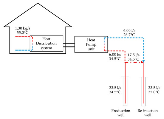
Figure 1.
Scheme of the system operation.
The sustainability of such geothermal exploitation has been analyzed by a numerical simulation, comprising a one fault case and two faults case, using the commercial software COMSOL Multiphysics® to assess the reservoir thermal perturbation (for 60 years of system operation for heating needs) due to extraction and reinjection of fluids at a rate suitable to produce the required thermal power.
Due to low enthalpy values and high water pressure effects on the reservoir, mechanical deformations have been considered negligible. A further element of interest in the modeling is due to the position of the wells (of the extraction/injection) in the plant. In fact, for logistical constraints, the injection well is not downstream of the extraction well, but almost flanked by this with respect to the flow direction of the groundwater body. The numerical results obtained allow development of a solid conceptual model for the Mondragone geothermal reservoir exploitation and open the possibility to future applications to similar geothermal reservoirs which are widespread in the Mediterranean region.
3. Hydrogeological Setting and Conceptual Model of the Geothermal Area
The area of interest is located on the coastal plain of Mondragone town at the bottom of Mt. Petrino carbonate hill (Figure 2).
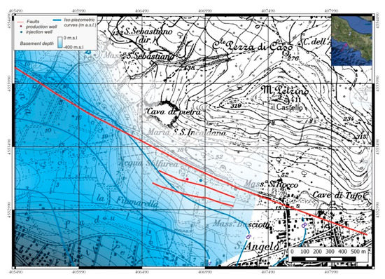
Figure 2.
Localization and hydrogeological structural setting of the analyzed site. (Adapted from [1]).
This is at SW of Mt. Massico, which is a carbonate monocline trending SW bounded by high-angle normal faults along the margins of the Garigliano (NW), Volturno (SE), and Mondragone (SW) plains. These faults, several kilometers deep, have a throw estimated to be hundreds of meters [57,58,59]. Recent geophysical data have provided information about the bedrock of Mondragone plain. It is made by limestone and marly-arenaceous rocks and affected by several faults. The most important fault of this area crosses the whole plain from NW to SE and it is here coupled to other sub-parallel faults. The carbonate bedrock near Mt. Petrino has been found at a depth of –30 m below ground level (b.g.l.), under pyroclastic-alluvial deposits. From this zone, moving towards SE, the bedrock shows instead a regular depth towards the sea [1] (Figure 2).
Boreholes’ data in the plain have shown the presence of a powerful bank of Campanian Ignimbrite tuff almost continuous across the plain. This tuff has low permeability and therefore separates the pyroclastic-alluvial aquifer (very poor) above the tuff, from the underlain alluvial deposits, deeper and more permeable, generating confined conditions in this lower aquifer. This last aquifer receives groundwater from lateral and vertical flows from the carbonate hill of Mt. Petrino, which is not hydro-geologically connected with the Mt. Massico, and from the carbonate bedrock, both shallow and deeper groundwater flow from NE to SW, toward the sea [22,60] (Figure 2).
Groundwater below the tuff presents interesting chemical characteristics: temperatures and average electrical conductivities are above 20 °C and >20,000 µS/cm, respectively, while, in the neighboring areas, these parameters show lower values (i.e., conductivity around 1000 µS/cm). These anomalies can be explained by the rise of deep mineralized waters (rich in gas, above all CO2 of inorganic origin [61]) along the faults of the carbonate bedrock. These deep waters mix with groundwater below the tuff and increase their total dissolved solids and temperature, features that are distributed along the groundwater flow direction [22].
Additional data about the mineralized zone is derived from drilling, in the frame of VIGOR project, of a geothermal exploration well, 300 m deep, about 150 m from the base of Mt. Petrino (Figure 2). The first 167 meters of the well stratigraphy (Table 2) highlight that limestone starts under pyroclastic-alluvial deposits at about 30 m b.g.l., and that fracturing of crossed carbonate rocks reaches its maximum around 100–120 m b.g.l. (Table 3).
Table 2.
Geothermal stratigraphy and geophysical properties of the layers composing the analyzed domain.
Table 3.
Temperatures and lithology of the geothermal exploration well at different depths.
Table 2 reports the geothermal stratigraphy and the geophysical properties of the layers composing the analyzed domain. Density, thermal conductivity, and porosity were derived from literature, whereas the permeability was determined through “Lugeon tests” performed at different depths in the exploration well.
The experimental campaign has revealed the presence of artesian groundwater (under a maximum pressure of 1.70 bars) in the carbonate rocks, from which, in absence of confinement, about 23.5 L/s naturally flow [1]. After reaching the depth of 300 m, inside the well (and with a temporary casing) geophysical logs were performed (using a probe 2PFA-1000 / MATRIX converter) to measure temperature (Table 3) and verticality. During drilling, groundwater samples have been collected at different depths to analyze changes in chemical composition. The gases have been also sampled at two different sites, in correspondence of the geothermal exploration well and in its vicinity [60]. It was found that the chemical characteristics of groundwater along the depth are similar; the gases sampled are 98% CO2, whose average concentration is 1380 mg/L [1,60].
Combining all data, a geothermal model that controls the mineralization of groundwater at the base of Mt. Petrino can be proposed [1,10,22,26,60,61]. According to this model, the geothermal reservoir corresponds to the carbonate bedrock of the Mondragone plain. Near Mt. Petrino, deep hot gases (mainly CO2) rise along the faults of the bedrock, involving groundwater (sodium-bicarbonate type) typical of a reducing environment and of meteoric origin. From the carbonate bedrock, thermo-mineral groundwater spreads in the overlying pyroclastic-alluvial aquifer diluting gradually. Therefore, the geothermal process is closely linked to the faults, as shown by temperature increase, which occurs, as measured continuously along the well (Table 3), at the same levels of major fracturing degree. Therefore, it is very likely that these levels represent the preferential path along which the hot fluid rise occurs [60,61].
4. Numerical Simulation of Geothermal Exploitation
In order to investigate the sustainability of geothermal exploitation, a numerical model was developed to analyze the coupled multiphase thermo-hydraulic processes due to the extraction and reinjection of groundwater. The model was implemented within the Finite Element commercial software COMSOL Multiphysics®, which is a powerful tool to reproduce coupled or multiphysics phenomena.
4.1. Governing Equations
Geothermal energy exploitation involves the interaction of different physical phenomena occurring in the ground, such as fluid flow, heat transport, chemical transport, and mechanical deformation [32,34,62]. In this work, only heat and fluid flow in fully saturated porous media were analyzed, considering the conservation laws of mass, momentum, and energy in a porous medium, that represents the ground.
The conservation of mass for a fluid flowing through a porous medium is expressed as:
where ρ is the fluid density, ε is the porosity, u is the seepage (Darcy) velocity vector. Therefore, the terms ρε and ρu represent the mass per unit volume within the porous matrix and the fluid mass flux, respectively. The flow velocity is low due to the low values of permeability and porosity of the domain. In this study, the porous medium flow was analyzed by using the well-known Darcy equation, which is the most common approach in geo-mechanic [63]. According to Darcy equation, the net flux across a face of porous surface, u, is linearly related to the pressure gradient, ∇p, as
where K is the permeability of the porous medium and µ the geothermal fluid dynamic viscosity. Since the fluid flow is coupled to heat transfer, the dependence of fluid properties on temperature is taken into account.
The Darcy’s flow model is coupled with heat transport in a porous medium to study the temperature distribution under geothermal exploitation. In the heat transport equation, the local thermal equilibrium between the solid and fluid phases is considered. Therefore, the solid temperature, Ts, is equal to the fluid temperature, Tf. Moreover, heat transport between solid and fluid phases is considered to be negligible. The heat transport in the subsurface is described as [64,65]
where cp is the specific heat, k is the thermal conductivity. The term (ρcp)eq represents the volumetric heat capacity of the porous medium. The subscript eq indicates that these are equivalent properties since they are spatially averaged to account for the porous matrix according to
where θp is the porous matrix volume fraction and subscript p indicates quantities that are related to the solid porous matrix.
4.2. Boundary and Initial Conditions
The boundary conditions employed in the present model refer to the ground and the well domains. For logistical reasons, the position of the injection well is not the traditional one, which is downstream of the extraction well [66]. The injection well is in fact placed, along the direction of groundwater flow, parallel to the extraction well and not far behind this (Figure 2). The top and bottom surfaces of the ground domain are considered impermeable to mass (u = 0), such as the lateral surfaces parallel to the groundwater flow. The average hydraulic gradient, (i), in the groundwater layer was estimated, according to Corniello et al. [22], with a NE–SW direction of the flow, determined from the iso-piezometric map of the area (Figure 2).
A prescribed velocity u was assigned on the filtering lateral surfaces of the wells. This value was calculated considering the water flow rate of extraction and injection, , measured during the experimental campaign. As initial condition for the groundwater flow equation, the hydraulic head, H, derived from experimental measurements, was imposed on the whole domain. The bottom ground surface was assumed to be adiabatic, whereas a convective heat flux is imposed on the top surface of the domain. The external temperature was assumed to be equal to 16.0 °C, which is the yearly average temperature of the area. As concerns the wells, a fixed temperature, T, equal to that of flow extraction and injection, is imposed on the lateral surfaces. The water temperature values measured along the exploration well [1,56] are illustrated in Figure 3. The soil was assumed to be in local thermal equilibrium with the groundwater, then the measured temperature profile (Table 3) was considered as the initial condition on the ground domain. All boundary and initial conditions are summarized in Figure 3 and Table 4.
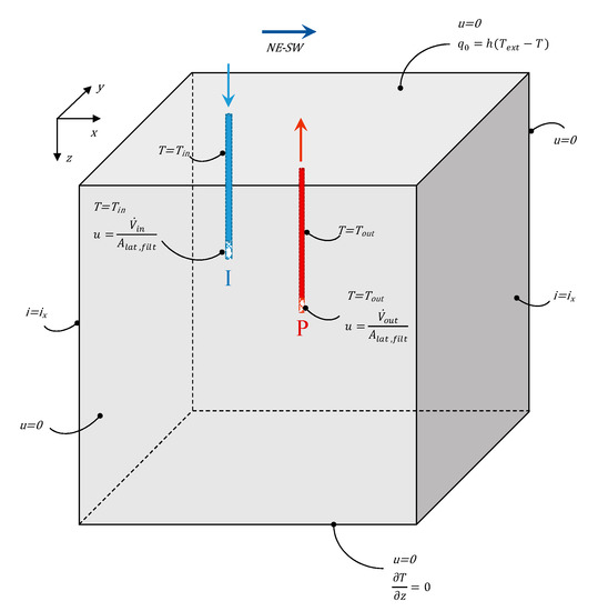
Figure 3.
Sketch of boundary and domain initial conditions (for clarity the width of the wells is enlarged). P and I represent the production and injection wells, respectively.
Table 4.
Boundary and initial conditions.
The experimental campaign revealed a sub-vertical fault zone, NW–SE oriented. The injection well is located at 135 m (Figure 2) from the production well, in the rearward direction. From the stratigraphical data of the exploration well, two different faults were found between 100–120 and 180–240 m b.g.l., according also to the results of the detailed geophysical survey. The deepest fault if projected towards the injection well may or may not meet this well at about 80 m depth. For this reason, two case studies were analyzed, one with the fault crossing the injection well and the other without. The fault zone presents the same characteristics of the layer identified by the number 10 in Table 2.
5. Results and Discussion
The numerical model described in the previous section was used to study the sustainable use of the low-temperature geothermal field of Mondragone. In order to evaluate the sustainability of this use, the temperature field in the ground was modeled over a period of time in which the source was continuously used at the full capacity of the plant. As mentioned above, the analysis was carried out with and without the fault zone crossing the injection well, to assess its influence on heat transfer and fluid flow. The simulations that refer to a single fault are indicated as Case 1 from now on, whereas those with the domain that includes two fault zones are referred to as Case 2. Figure 4 shows a schematic representation of the domain considered for the analysis of Case 1 where a single fault, indicated as F1, is present. In Case 2 the domain is the same, with the addition of a fault zone crossing the injection well, as shown in Figure 5. For the sake of clarity, only the data concerning the fault crossing the injection well, indicated as F2, are reported in Figure 5.
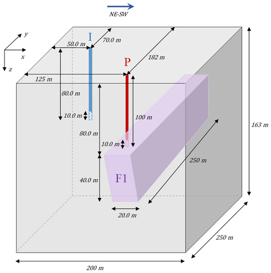
Figure 4.
Computational domain in the case of a single fault (F1).
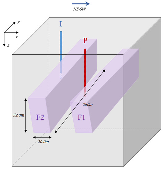
Figure 5.
Computational domain in the case of double faults (F1 and F2).
The overall domain is defined as a rectangular parallelepiped of 163 m in depth with a basis equal to 250 × 200 m. Below this depth, the effect of the geothermal system is considered negligible due to the lower degree of fracturing in limestone. The fault zones have both a thickness of 20.0 m and a slope of 10° in relation to the vertical axis. The production and reinjection wells cross the fault cataclastic zone starting from 80.0 to 120 and 68.0 to 110 m b.g.l., respectively. Both the wells have a radius of 24.4 cm and a filtering section of 10.0 m in height from the top of the cataclastic zones.
The water properties, ρ, µ, cp, and k are considered temperature-dependent. For the ground domain, literature values of thermal conductivity, density, porosity, and permeability of the eight layers found during the well drilling were considered. The parameters used in the numerical simulation are reported in Table 4.
A 3D unstructured mesh, refined near all the boundaries to capture the larger gradients of both flow velocity and temperature, was used. Indeed, the grid needs to be finer in the region of greatest change in the skin zone close to the well and can be coarser further out in the reservoir [67]. For the sake of clarity, the mesh used for the case of a single fault is reported in Figure 6.
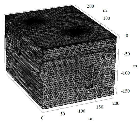
Figure 6.
Mesh used to analyze the case of a single fault.
The details of the meshes used for the two cases are shown in Table 5. A mesh sensitivity study was carried out to obtain grid-independent results from the calculations.
Table 5.
Mesh details for Case 1 (single fault) and Case 2 (two faults).
In order to assess the impact of the geothermal exploitation on the ground domain, the groundwater velocity field and the ground temperature field were determined through the proposed model for a period of time of 60 years.
The temperature fields at different times in the xz plan cutting the domain in correspondence of the two wells’ axes are reported in Figure 7 for the case of the single fault (Case 1) and in Figure 8 for the case of double (Case 2) fault zones. For the sake of clarity, the section cuts are also reported.
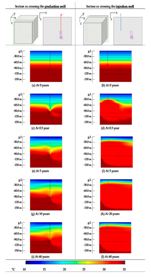
Figure 7.
Temperature field of the sections xz crossing the wells, at different times, for Case 1 (single fault).
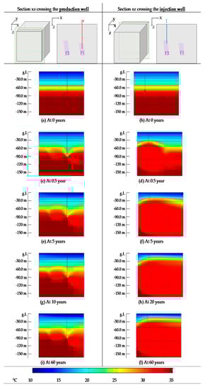
Figure 8.
Temperature field of the sections xz crossing the wells, at different times, for Case 2 (double faults).
The effect of geothermal extraction is mainly contained in the area surrounding the production well. A moderate decrease in the ground temperature can be observed in the downstream region: the variation is similar in both Cases 1 and 2.
In the upstream section the temperature field remains almost unchanged in Case 1, whereas in Case 2 a temperature decrease can be observed in the region delimited by the two faults. The difference is due to the permeability and the thermal conductivity of the fault zone, which are larger than those of the surrounding material. However, in both cases after 10 years of operation the temperature field does not change any more (reaching steady state operation of the reservoir). The effect of injection is more pronounced than that of extraction in both cases. However, the thermal disturbance does not reach the superficial layers, since it is limited by the 5th layer which has lower values of permeability and thermal conductivity with respect to the other layers (Table 2). The injection in the fault slightly modifies the temperature distribution within the domain: the propagation of the thermal disturbance is lower in layers over the fault and higher towards the bottom of the domain. In both cases, the temperature field does not change any more after 20 years of operation, therefore the period of time needed to reach a steady condition is longer in the region surrounding the injection well than in the area of the production well. This is probably due to the higher difference in temperature between groundwater surrounding the injection well and injected water.
The temperature field, at different times, in the yz plan cutting the domain in correspondence of the axis of two wells is shown in Figure 9 and Figure 10 for Cases 1 and 2, respectively. For the sake of clarity, the section cuts are also reported. In these plots, it can be noticed that the temperature decrease caused by the injection well is localized in the region of the domain behind the production well and it is less pronounced in Case 1. In Case 1 the temperature propagation is more pronounced towards the upper layers, whereas in Case 2 it is larger in the bottom of the domain.
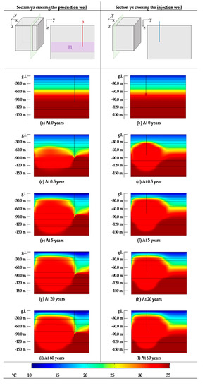
Figure 9.
Temperature field of the sections yz crossing the wells, at different times, for Case 1 (single fault).
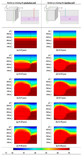
Figure 10.
Temperature field of the sections yz crossing the wells, at different times, for Case 2 (double faults).
The temperature distribution and the streamlines indicating the velocity field, at different depths and times, reported in Figure 11, clearly show that the direction of the thermal disturbance is significantly influenced by the groundwater flow. A stable temperature distribution is reached after 25 years at the lowest depths, whereas only 5 years are needed at highest depths. The thermal disturbance in the layer close to the top surface of the domain is concentrated in the region surrounding the injection well.
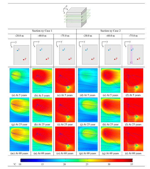
Figure 11.
Temperature field at different depths and times, for Case 1 (single fault) and Case 2 (two faults).
The fault located in correspondence of the injection well, F2, does not significantly affect the temperature distribution, except for the upstream region of the production well, where the temperature is slightly lower than in Case 1. Conversely, the fault influences the velocity field, due to the permeability, which is larger than in the adjacent layers. This variation in the velocity field is mainly responsible for the extension of the region affected by the thermal disturbance in Case 2.
At depths below 75.0 m from ground level the temperature and velocity fields are constant over time, therefore only their variation with depth was taken into account. Analyzing the plots in Figure 12, which are all related to the time of 60 years, it can be observed that the thermal disturbance is more extended in Case 2. In addition, at 155 m b.g.l. the thermal disturbance can be neglected in Case 1, whereas in Case 2 the region downstream of the injection well is still affected by the geothermal exploitation.
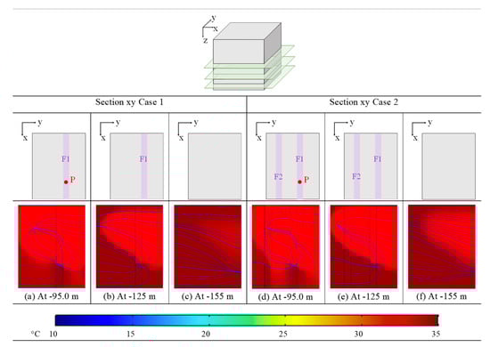
Figure 12.
Temperature field at different depths, for Case 1 (single fault) and Case 2 (two faults).
The Darcy velocity field and magnitude at different depths for Cases 1 and 2 are reported in Figure 13 and Figure 14, respectively. The xy sections reported in these figures are related to different layers of the domain, in order to analyze the influence of their properties on the groundwater flow. In the first two layers of the domain, (refer to Figure 13a,b and Figure 14a,b), both the distribution and the magnitude of Darcy velocity do not change from Case 1 to Case 2, and result as constant in the entire xy plans considered. This is due to the low permeability of the third layer, which avoids the effect of the geothermal exploitation on the groundwater flow reaching the top of the domain. Indeed, the groundwater flow in the lower layers of the domain, which are characterized by higher values of permeability, varies in the regions where the production and injection wells are located (refer to Figure 13c,d and Figure 14c,d).
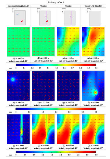
Figure 13.
Darcy velocity field at different depths for Case 1 (single fault).
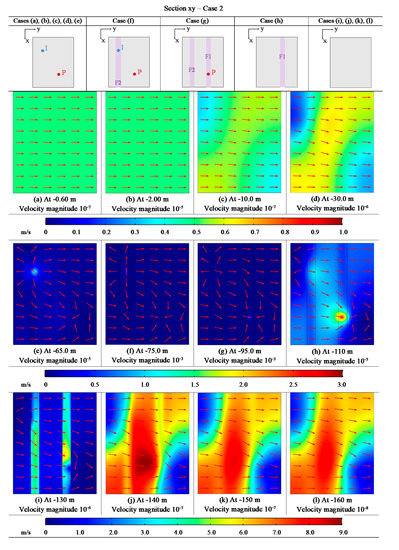
Figure 14.
Darcy velocity field at different depths for Case 2 (two faults).
Considering the injection well, the velocity magnitude decreases upstream and increases downstream, whereas the opposite trend can be observed in the region surrounding the production well. In Case 2, a lower propagation of the fluid flow disturbance can be observed: this is due to higher permeability of the material in the correspondence of the fault, which facilitates the groundwater flow, which is more concentrated in the tectonic region. In addition, considering Case 2, the velocity magnitude varies differently in the zones of injection and production, probably due to the different vertical extension of the faults. The fault located in the injection area, F2, is more extended and its effect on the upper layers is larger.
In the sections that cut the wells (refer to Figure 13f,g and Figure 14f,g), the Darcy velocity field and magnitude are similar in Case 1 and Case 2. Obviously, the magnitude is significantly higher than at other depths due to the flow extraction and injection. A different trend can be observed in sections 10.0 m distant from the bottom of the wells in the vertical direction (refer to Figure 13e,h and Figure 14e,h), mainly in the areas surrounding the injection well. The fault affects the groundwater flow, whose magnitude increases in the area surrounding the injection well and decreases upstream of the production well. However, a vertical distance of 10.0 m is sufficient to observe a significant decrease in the Darcy velocity, which tends to the undisturbed value as the horizontal distance from the wells increases. At higher depths, the velocity magnitude continues to decrease (refer to Figure 13i,l and Figure 14i,l). The velocity magnitude is higher in the central region of the considered section, where the groundwater has the same direction of the undisturbed fluid flow in both cases, injection and extraction.
Finally, in Figure 15, the temperature over time is plotted at three different distances from the wells (10, 50, and 100 m) at a depth equal to half of the filtering sections of the wells, for the two cases analyzed.
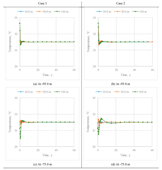
Figure 15.
Temperature over time at three different distances from the wells (10.0, 50.0, and 100 m), for two different depths (−95.0 and −75.0m).
Considering the production well (see Figure 15a,b) whose filtering section goes from −90 to −100 m, the geothermal exploitation causes a temperature decrease of around 2 °C during the considered period of time. The temperature becomes constant after 10 years in Case 1 and 20 years in Case 2. It is worth noticing that in Case 2, the temperature decrease at a distance of 100 m is slightly lower than in Case 1, suggesting a positive effect of the injection in the fault. A similar conclusion can be drawn analyzing the results related to the injection well (see Figure 15c,d). The variation in temperature with respect to the initial condition is lower than 1 °C, therefore significantly lower than that observed in the region of the production well. The period of time needed to reach a constant temperature is longer than for the production well: 20 years for the Case 1 and 25 years for the Case 2. The injection in the fault has a positive effect, reducing the temperature oscillations during the first years of exploitation in Case 2. The low decrease of the basin temperature is coherent with the results found in the literature related to the geothermal exploitation of low-temperature reservoirs [2].
So far, the numerical results show that the geothermal exploitation modifies the groundwater flow in correspondence with the filtering sections of the wells, whereas only a weak effect can be observed in the rest of the domain, in terms of speed and direction. In order to account for the possible presence of a fault crossing the injection well, two case studies were analyzed. When the injection occurs in the fault the variation of the velocity field is lower, thanks to the permeability in correspondence with the fault. The injection in the fault positively affects the temperature distribution as well. The thermal disturbance does not reach the top layers of the domain due to their hydraulic and thermal properties in both cases. It is worth noticing that in the case of injection in the fault the disturbance tends to be more concentrated in the same fault region, decreasing its effect on the other layers of the domain. In addition, in this case, also the temperature oscillation over time observed at the depth of the wells is lower than in the case without the injection in the fault.
The proposed model allows estimation of the effect of geothermal exploitation not only on the reservoir but also on the operation of the technological system that uses the geothermal source for thermal energy production. The results of the simulations indicate a temperature decrease of around 2.00 °C in the extraction temperature during the considered period of time. Such a decrease will reduce the thermal energy available from geothermal exploitation. In the specific case analyzed in this work, where a heat pump was considered to supply heat to two schools, a decrease in the COP of the heat pump is expected.
6. Conclusions
The numerical results on the geothermal exploitation here reported are of global interest for the following reasons: (a) the nature of aquifer represented by carbonate rocks with strong anisotropy, due to the presence of several fault systems, with confined groundwater; (b) the environmental effects of an open-loop well-doublet plant are assessed considering the geometry of the wells (imposed by logistical constraints) which is designed in a different way from the one usually adopted, where the injection well is placed downstream of the extraction well. In fact, even if thermal feedback is present at the production well due to the position of injection well, the sustainability of the use of the geothermal resource over time (60 years here tested) is asserted by the numerical simulation. In fact, the main results show that the temperature decrease is only 2.00 °C in correspondence with the production well filtering section, and even less at greater depths.
It is likely that the sustainability is linked, considering the hydrogeological scheme, to the characteristics of groundwater flow (direction and pressure) and to the position of the filtering section of the extraction well, that is placed near the main cataclastic zone of a fault along which the permeability is higher than the surrounding rocks and the upwelling of deep hot fluids is easier.
Even assuming the presence of another fault at the injection well, the numerical simulation still indicates the full sustainability of the geothermal plant. It is worth noticing that in the case of injection in the fault the disturbance tends to be more concentrated in the same fault region, decreasing its effect on the other layers of the domain. Finally, in all the cases considered, the thermal disturbance does not reach the top of the domain due to the hydraulic and thermal properties of the rocks closest to the ground level.
The definition of the hydrogeological and stratigraphic scheme of the geothermal area together with the numerical modelling are therefore decisive either for the final choice of the well plant localization or for the evaluation over time of the environment effects of the use of the geothermal resource in faulted carbonate rocks, which are common in Southern Italy and peri-Mediterranean regions.
Author Contributions
Conceptualization, M.I., N.M., and L.V.; Data curation, M.I. and A.C. (Alfonso Corniello); Formal analysis, S.D.F.; Funding acquisition, M.I., A.C. (Alberto Carotenuto), N.M., and L.V.; Methodology, S.D.F. and N.M.; Project administration, M.I., A.C. (Alberto Carotenuto) and N.M.; Writing—original draft, S.D.F.; Writing—review and editing, M.I., A.C. (Alberto Carotenuto), A.C. (Alfonso Corniello), S.D.F., N.M., R.S., L.V., and A.M. All authors have read and agreed to the published version of the manuscript.
Funding
The authors gratefully acknowledge the financial support of VIGOR project (Valutazione del Potenziale Geotermico delle Regioni Convergenza) CUP: B72J10000060007, GEOGRID project CUP: B43D18000230007 and project M027061 funded by Italian Ministry of the Foreign Affairs.
Conflicts of Interest
The authors declare no conflict of interest. The funders had no role in the design of the study; in the collection, analyses, or interpretation of data; in the writing of the manuscript, or in the decision to publish the results.
References
- Amoresano, A.; Angelino, A.; Anselmi, M.; Bianchi, B.; Botteghi, S.; Brandano, M.; Brilli, M.; Bruno, P.P.; Caielli, G.; Caputi, A.; et al. VIGOR: Sviluppo geotermico nella regione Campania—Studi di Fattibilità a Mondragone e Guardia Lombardi. In Progetto VIGOR—Valutazione del Potenziale Geotermico delle Regioni della Convergenza, POI Energie Rinnovabili e Risparmio Energetico 2007-2013; CNR-IGG: Pisa, Italy, 2014; ISBN 9788879580151. [Google Scholar]
- Kiryukhin, A.V.; Vorozheikina, L.A.; Voronin, P.O.; Kiryukhin, P.A. Thermal and permeability structure and recharge conditions of the low temperature Paratunsky geothermal reservoirs in Kamchatka, Russia. Geothermics 2017, 70, 47–61. [Google Scholar] [CrossRef]
- Manni, M.; Coccia, V.; Nicolini, A.; Marseglia, G.; Petrozzi, A. Towards zero energy stadiums: The case study of the Dacia arena in Udine, Italy. Energies 2018, 11, 2396. [Google Scholar] [CrossRef]
- Bonati, A.; De Luca, G.; Fabozzi, S.; Massarotti, N.; Vanoli, L. The integration of exergy criterion in energy planning analysis for 100% renewable system. Energy 2019, 174, 749–767. [Google Scholar] [CrossRef]
- Østergaard, P.A.; Lund, H. A renewable energy system in Frederikshavn using low-temperature geothermal energy for district heating. Appl. Energy 2011, 88, 479–487. [Google Scholar] [CrossRef]
- Kiryukhin, A.V.; Asaulova, N.P.; Vorozheikina, L.A.; Obora, N.V.; Voronin, P.O.; Kartasheva, E.V. Recharge Conditions of the Low Temperature Paratunsky Geothermal Reservoir, Kamchatka, Russia. Procedia Earth Planet. Sci. 2017, 17, 132–135. [Google Scholar] [CrossRef]
- Pocasangre, C.; Fujimitsu, Y.; Nishijima, J. Interpretation of gravity data to delineate the geothermal reservoir extent and assess the geothermal resource from low-temperature fluids in the Municipality of Isa, Southern Kyushu, Japan. Geothermics 2020, 83, 101735. [Google Scholar] [CrossRef]
- Zimmermann, G.; Moeck, I.; Blöcher, G. Cyclic waterfrac stimulation to develop an Enhanced Geothermal System (EGS)—Conceptual design and experimental results. Geothermics 2010, 39, 59–69. [Google Scholar] [CrossRef]
- Chen, Y.; Ma, G.; Wang, H.; Li, T.; Wang, Y.; Sun, Z. Optimizing heat mining strategies in a fractured geothermal reservoir considering fracture deformation effects. Renew. Energy 2020, 148, 326–337. [Google Scholar] [CrossRef]
- Simsek, S. Hydrogeological and isotopic survey of geothermal fields in the Buyuk Menderes graben, Turkey. Geothermics 2003, 32, 669–678. [Google Scholar] [CrossRef]
- Gouasmia, M.; Gasmi, M.; Mhamdi, A.; Bouri, S.; Dhia, H.B. Prospection géoélectrique pour l’étude de l’aquifère thermal des calcaires récifaux, Hmeïma–Boujabeur (Centre ouest de la Tunisie). Comptes Rendus Geosci. 2006, 338, 1219–1227. [Google Scholar] [CrossRef]
- Mohammadi, Z.; Bagheri, R.; Jahanshahi, R. Hydrogeochemistry and geothermometry of Changal thermal springs, Zagros region, Iran. Geothermics 2010, 39, 242–249. [Google Scholar] [CrossRef]
- Duan, Z.; Pang, Z.; Wang, X. Sustainability evaluation of limestone geothermal reservoirs with extended production histories in Beijing and Tianjin, China. Geothermics 2011, 40, 125–135. [Google Scholar] [CrossRef]
- Pasquale, V.; Verdoya, M.; Chiozzi, P. Heat flow and geothermal resources in northern Italy. Renew. Sustain. Energy Rev. 2014, 36, 277–285. [Google Scholar] [CrossRef]
- Homuth, S.; Götz, A.; Sass, I. Reservoir characterization of the Upper Jurassic geothermal target formations (Molasse Basin, Germany): Role of thermofacies as exploration tool. Geotherm. Energy Sci. 2015, 3, 41–49. [Google Scholar] [CrossRef]
- Montanari, D.; Minissale, A.; Doveri, M.; Gola, G.; Trumpy, E.; Santilano, A.; Manzella, A. Geothermal resources within carbonate reservoirs in western Sicily (Italy): A review. Earth-Sci. Rev. 2017, 169, 180–201. [Google Scholar] [CrossRef]
- Cataldi, R.; Mongelli, F.; Squarci, P.; Taffi, L.; Zito, G.; Calore, C. Geothermal ranking of Italian territory. Geothermics 1995, 1, 115–129. [Google Scholar] [CrossRef]
- Minissale, A.; Duchi, V. Geothermometry on fluids circulating in a carbonate reservoir in north-central Italy. J. Volcanol. Geotherm. Res. 1988, 35, 237–252. [Google Scholar] [CrossRef]
- Della Vedova, B.; Bellani, S.; Pellis, G.; Squarci, P. Deep temperatures and surface heat flow distribution. In Anatomy of An Orogen: The Apennines and Adjacent Mediterranean Basins; Springer: Berlin/Heidelberg, Germany, 2001; pp. 65–76. [Google Scholar]
- Chiarabba, C.; Chiodini, G. Continental delamination and mantle dynamics drive topography, extension and fluid discharge in the Apennines. Geology 2013, 41, 715–718. [Google Scholar] [CrossRef]
- Giambastiani, B.; Tinti, F.; Mendrinos, D.; Mastrocicco, M. Energy performance strategies for the large scale introduction of geothermal energy in residential and industrial buildings: The GEO. POWER project. Energy Policy 2014, 65, 315–322. [Google Scholar] [CrossRef]
- Corniello, A.; Cardellicchio, N.; Cavuoto, G.; Cuoco, E.; Ducci, D.; Minissale, A.; Mussi, M.; Petruccione, E.; Pelosi, N.; Rizzo, E.; et al. Hydrogeological Characterization of a Geothermal system: The case of the Thermo-mineral area of Mondragone (Campania, Italy). Int. J. Environ. Res. 2015, 9, 523–534. [Google Scholar]
- Taillefer, A.; Soliva, R.; Guillou-Frottier, L.; Le Goff, E.; Martin, G.; Seranne, M. Fault-related controls on upward hydrothermal flow: An integrated geological study of the têt fault system, eastern pyrénées (France). Geofluids 2017, 2017, 8190109. [Google Scholar] [CrossRef]
- Chi, G.; Xue, C. An overview of hydrodynamic studies of mineralization. Geosci. Front. 2011, 2, 423–438. [Google Scholar] [CrossRef]
- Lowell, R.P.; Farough, A.; Hoover, J.; Cummings, K. Characteristics of magma-driven hydrothermal systems at oceanic spreading centers. Geochem. Geophys. Geosystems 2013, 14, 1756–1770. [Google Scholar] [CrossRef]
- Lowell, R.P. A fault-driven circulation model for the Lost City Hydrothermal Field. Geophys. Res. Lett. 2017, 44, 2703–2709. [Google Scholar] [CrossRef]
- Moeck, I.S. Catalog of geothermal play types based on geologic controls. Renew. Sustain. Energy Rev. 2014, 37, 867–882. [Google Scholar] [CrossRef]
- Blöcher, G.; Cacace, M.; Reinsch, T.; Watanabe, N. Evaluation of three exploitation concepts for a deep geothermal system in the North German Basin. Comput. Geosci. 2015, 82, 120–129. [Google Scholar] [CrossRef]
- Calise, F.; Di Fraia, S.; Macaluso, A.; Massarotti, N.; Vanoli, L. A geothermal energy system for wastewater sludge drying and electricity production in a small island. Energy 2018, 163, 130–143. [Google Scholar] [CrossRef]
- Di Fraia, S.; Macaluso, A.; Massarotti, N.; Vanoli, L. Energy, exergy and economic analysis of a novel geothermal energy system for wastewater and sludge treatment. Energy Convers. Manag. 2019, 195, 533–547. [Google Scholar] [CrossRef]
- Franco, A.; Vaccaro, M. Numerical simulation of geothermal reservoirs for the sustainable design of energy plants: A review. Renew. Sustain. Energy Rev. 2014, 30, 987–1002. [Google Scholar] [CrossRef]
- Carotenuto, A.; Massarotti, N.; Mauro, A. A new methodology for numerical simulation of geothermal down-hole heat exchangers. Appl. Therm. Eng. 2012, 48, 225–236. [Google Scholar] [CrossRef]
- Carotenuto, A.; Ciccolella, M.; Massarotti, N.; Mauro, A. Models for thermo-fluid dynamic phenomena in low enthalpy geothermal energy systems: A review. Renew. Sustain. Energy Rev. 2016, 60, 330–355. [Google Scholar] [CrossRef]
- Carotenuto, A.; Marotta, P.; Massarotti, N.; Mauro, A.; Normino, G. Energy piles for ground source heat pump applications: Comparison of heat transfer performance for different design and operating parameters. Appl. Therm. Eng. 2017, 124, 1492–1504. [Google Scholar] [CrossRef]
- Sanyal, S.K.; Butler, S.J.; Swenson, D.; Hardeman, B. Review of the state-of-the-art of numerical simulation of enhanced geothermal systems. In Proceedings of the World Geothermal Congress 2000, Kyushu, Japan, 28 May–10 June 2000. [Google Scholar]
- Burnell, J.; Clearwater, E.; Croucher, A.; Kissling, W.; O’Sullivan, J.; O’Sullivan, M.; Yeh, A. Future directions in geothermal modelling. In Proceedings of the (Electronic) 34rd New Zealand Geothermal Workshop, Auckland City, New Zealand, 19–21 November 2012. [Google Scholar]
- White, J.A.; Foxall, W. Assessing induced seismicity risk at CO2 storage projects: Recent progress and remaining challenges. Int. J. Greenh. Gas Control 2016, 49, 413–424. [Google Scholar] [CrossRef]
- Moridis, G.J.; Pruess, K. T2SOLV: An enhanced package of solvers for the TOUGH2 family of reservoir simulation codes. Geothermics 1998, 27, 415–444. [Google Scholar] [CrossRef]
- O’Sullivan, M.J.; Pruess, K.; Lippmann, M.J. State of the art of geothermal reservoir simulation. Geothermics 2001, 30, 395–429. [Google Scholar] [CrossRef]
- O’Sullivan, M.J.; Yeh, A.; Mannington, W.I. A history of numerical modelling of the Wairakei geothermal field. Geothermics 2009, 38, 155–168. [Google Scholar] [CrossRef]
- Bujakowski, W.; Barbacki, A.; Miecznik, M.; Pająk, L.; Skrzypczak, R.; Sowiżdżał, A. Modelling geothermal and operating parameters of EGS installations in the lower triassic sedimentary formations of the central Poland area. Renew. Energy 2015, 80, 441–453. [Google Scholar] [CrossRef]
- Carlino, S.; Troiano, A.; Di Giuseppe, M.G.; Tramelli, A.; Troise, C.; Somma, R.; De Natale, G. Exploitation of geothermal energy in active volcanic areas: A numerical modelling applied to high temperature Mofete geothermal field, at Campi Flegrei caldera (Southern Italy). Renew. Energy 2016, 87, 54–66. [Google Scholar] [CrossRef]
- Zyvoloski, G.; Dash, Z.; Kelkar, S. FEHMN 1.0: Finite Element Heat and Mass Transfer Code; Los Alamos National Lab: Los Alamos, NM, USA, 1992. [Google Scholar]
- Zyvoloski, G. FEHM: A control volume finite element code for simulating subsurface multi-phase multi-fluid heat and mass transfer. In Los Alamos Unclassified Report LA-UR-07-3359; Los Alamos National Lab: Los Alamos, NM, USA, 2007. [Google Scholar]
- Kelkar, S.; Lewis, K.; Karra, S.; Zyvoloski, G.; Rapaka, S.; Viswanathan, H.; Mishra, P.; Chu, S.; Coblentz, D.; Pawar, R. A simulator for modeling coupled thermo-hydro-mechanical processes in subsurface geological media. Int. J. Rock Mech. Min. Sci. 2014, 70, 569–580. [Google Scholar] [CrossRef]
- Dempsey, D.; Kelkar, S.; Davatzes, N.; Hickman, S.; Moos, D. Numerical modeling of injection, stress and permeability enhancement during shear stimulation at the Desert Peak Enhanced Geothermal System. Int. J. Rock Mech. Min. Sci. 2015, 78, 190–206. [Google Scholar] [CrossRef]
- Faust, C.R.; Mercer, J.W. Geothermal reservoir simulation: 1. Mathematical models for liquid-and vapor-dominated hydrothermal systems. Water Resour. Res. 1979, 15, 25–30. [Google Scholar] [CrossRef]
- Higuchi, S.; Nishijima, J.; Fujimitsu, Y. Integration of geothermal exploration data and numerical simulation data using GIS in a hot spring area. Procedia Earth Planet. Sci. 2013, 6, 177–186. [Google Scholar] [CrossRef]
- Pola, M.; Fabbri, P.; Piccinini, L.; Zampieri, D. Conceptual and numerical models of a tectonically-controlled geothermal system: A case study of the Euganean Geothermal System, Northern Italy. Cent. Eur. Geol. 2015, 58, 129–151. [Google Scholar] [CrossRef]
- Aliyu, M.D.; Chen, H.-P. Optimum control parameters and long-term productivity of geothermal reservoirs using coupled thermo-hydraulic process modelling. Renew. Energy 2017, 112, 151–165. [Google Scholar] [CrossRef]
- Bakhsh, K.J.; Nakagawa, M.; Arshad, M.; Dunnington, L. Modeling thermal breakthrough in sedimentary geothermal system, using COMSOL multiphysics. In Proceedings of the 41st Workshop on Geothermal Reservoir Engineering, Stanford, CA, USA, 22–24 February 2016. [Google Scholar]
- Romano-Perez, C.; Diaz-Viera, M. A Comparison of Discrete Fracture Models for Single Phase Flow in Porous Media by COMSOL Multiphysics® Software. In Proceedings of the 2015 COMSOL Conference in Boston, Boston, MA, USA, 7–9 October 2012. [Google Scholar]
- Pandey, S.; Chaudhuri, A.; Kelkar, S. A coupled thermo-hydro-mechanical modeling of fracture aperture alteration and reservoir deformation during heat extraction from a geothermal reservoir. Geothermics 2017, 65, 17–31. [Google Scholar] [CrossRef]
- Pandey, S.; Chaudhuri, A.; Kelkar, S.; Sandeep, V.; Rajaram, H. Investigation of permeability alteration of fractured limestone reservoir due to geothermal heat extraction using three-dimensional thermo-hydro-chemical (THC) model. Geothermics 2014, 51, 46–62. [Google Scholar] [CrossRef]
- Cherubini, Y.; Cacace, M.; Blöcher, G.; Scheck-Wenderoth, M. Impact of single inclined faults on the fluid flow and heat transport: Results from 3-D finite element simulations. Environ. Earth Sci. 2013, 70, 3603–3618. [Google Scholar] [CrossRef]
- Carotenuto, A.; De Luca, G.; Fabozzi, S.; Figaj, R.D.; Iorio, M.; Massarotti, N.; Vanoli, L. Energy analysis of a small geothermal district heating system in Southern Italy. Int. J. Heat Technol. 2016, 34, S519–S527. [Google Scholar] [CrossRef]
- Billi, A.; Bosi, V.; De Meo, A. Caratterizzazione strutturale del rilievo del M. Massico nell’ambito dell’evoluzione quaternaria delle depressioni costiere dei fiumi Garigliano e Volturno (Campania Settentrionale). Il Quat. 1997, 10, 15–26. [Google Scholar]
- Milia, A.; Torrente, M.M. Tectono-stratigraphic signature of a rapid multistage subsiding rift basin in the Tyrrhenian-Apennine hinge zone (Italy): A possible interaction of upper plate with subducting slab. J. Geodyn. 2015, 86, 42–60. [Google Scholar] [CrossRef]
- Luiso, P.; Paoletti, V.; Nappi, R.; La Manna, M.; Cella, F.; Gaudiosi, G.; Fedi, M.; Iorio, M. A multidisciplinary approach to characterize the geometry of active faults: The example of Mt. Massico, Southern Italy. Geophys. J. Int. 2018, 213, 1673–1681. [Google Scholar] [CrossRef]
- Corniello, A.; Ducci, D.; Ruggieri, G.; Iorio, M. Complex groundwater flow circulation in a carbonate aquifer: Mount Massico (Campania Region, Southern Italy). Synergistic hydrogeological understanding. J. Geochem. Explor. 2018, 190, 253–264. [Google Scholar] [CrossRef]
- Cuoco, E.; Minissale, A.; Tamburrino, S.; Iorio, M.; Tedesco, D. Fluid geochemistry of the Mondragone hydrothermal systems (southern Italy): Water and gas compositions vs. geostructural setting. Int. J. Earth Sci. 2017, 106, 2429–2444. [Google Scholar] [CrossRef]
- Adinolfi, M.; Maiorano, R.M.S.; Mauro, A.; Massarotti, N.; Aversa, S. On the influence of thermal cycles on the yearly performance of an energy pile. Geomech. Energy Environ. 2018, 16, 32–44. [Google Scholar] [CrossRef]
- Di Fraia, S.; Massarotti, N.; Nithiarasu, P. Modelling electro-osmotic flow in porous media: A review. Int. J. Numer. Methods Heat Fluid Flow 2018, 28, 472–497. [Google Scholar] [CrossRef]
- Arpino, F.; Carotenuto, A.; Ciccolella, M.; Cortellessa, G.; Massarotti, N.; Mauro, A. Transient natural convection in partially porous vertical annuli. Int. J. Heat Technol. 2016, 34, S512–S518. [Google Scholar] [CrossRef]
- Massarotti, N.; Ciccolella, M.; Cortellessa, G.; Mauro, A. New benchmark solutions for transient natural convection in partially porous annuli. Int. J. Numer. Methods Heat Fluid Flow 2016, 26, 1187–1225. [Google Scholar] [CrossRef]
- Banks, D. Thermogeological assessment of open-loop well-doublet schemes: A review and synthesis of analytical approaches. Hydrogeol. J. 2009, 17, 1149–1155. [Google Scholar] [CrossRef]
- McLean, K.; Zarrouk, S.J. Pressure transient analysis of geothermal wells: A framework for numerical modelling. Renew. Energy 2017, 101, 737–746. [Google Scholar] [CrossRef]


© 2020 by the authors. Licensee MDPI, Basel, Switzerland. This article is an open access article distributed under the terms and conditions of the Creative Commons Attribution (CC BY) license (http://creativecommons.org/licenses/by/4.0/).