Abstract
The underground air tunnel system shows promising potentials for reducing energy consumption of buildings and for improving indoor thermal comfort, whereas the existing dynamic models using the computational fluid dynamic (CFD) method show computational complexity and are user-unfriendly for parametrical analysis. In this study, a dynamic numerical model was developed with the on-site experimental calibration. Compared to the traditional CFD method with high computational complexity, the mathematical model on the MATLAB/SIMULINK platform is time-saving in terms of the real-time thermal performance prediction. The experimental validation results indicated that the maximum absolute relative deviation was 3.18% between the model-driven results and the data from the on-site experiments. Parametrical analysis results indicated that, with the increase of the tube length, the outlet temperature decreases with an increase of the cooling capacity whereas the increasing/decreasing magnitude slows down. In addition, the system performance is independent on the tube materials. Furthermore, the outlet air temperature and cooling capacity are dependent on the tube diameter and air velocity, i.e., a larger tube diameter and a higher air velocity are more suitable to improve the system’s cooling capacity, and a smaller tube diameter and a lower air velocity will produce a more stable and lower outlet temperature. Further studies need to be conducted for the trade-off solutions between air velocity and tube diameter for the bi-criteria performance enhancement between outlet temperature and cooling capacity. This study proposed an experimentally validated mathematical model to accurately predict the thermal performance of the underground air tunnel system with high computational efficiency, which can provide technical guidance to multi-combined solutions through geometrical designs and operating parameters for the optimal design and robust operation.
1. Introduction
As a considerable energy consumer, building energy consumption has become one of the three major energy users all around the world, accounting for more than 30% of the total global energy consumptions [1,2,3]. In China, the energy consumption in buildings increases every year, especially with social development and the improvement of living conditions. The considerable building energy consumptions require high dependence on fossil fuels, which will result in deteriorated environmental concerns [4,5]. The contradiction between the daily increased energy demand and the energy shortage calls for the necessity to deploy renewable energy [6,7,8,9] and to reduce the dependence on fossil fuels. In order to reduce the reliance on traditional fossil fuels without sacrificing economic and social development, the deployment of large-scale renewable energy systems (such as heating, cooling, and electric systems) has become one of the most promising solutions to reduce the building energy consumption and to cover the building demand [10,11]. Depending on the renewable energy sources, the renewable energy systems can be classified into solar-driven [12,13,14,15,16,17], wind-driven, and geothermal-driven energy systems. Compared to the instability in temporal distribution and the unevenness in spatial distribution of solar and wind resources, the geothermal energy shows promising potentials in terms of the abundant resource distribution, the stability of energy supply, the simplicity of system designs and operations, and so on. Geothermal energy has attracted increasing interests with prioritized recommendations for regulating indoor and built environments and for reducing building energy consumptions [18,19,20]. The underlying mechanism for the application the geothermal energy in buildings is that, due to the high thermal inertia of underground soil, independent of the ambient air temperature, solar radiation, and water flows, the soil temperature (3–4 m beneath the ground) normally remains relatively constant during the whole year. The relatively steady soil temperature is promising when being utilized as a “heat sink” or “heating source” for space cooling in summer or as a space heater in winter [21,22].
The underground air tunnel (UAT) system, as one of the most widely used geothermal energy technologies, has attracted more and more interests for reducing energy consumption of buildings [23,24], especially in areas where geothermal energy can be highly recommended. The UAT system is also called the earth-to-air heat exchanger (EAHE), the air–soil heat exchanger (ASHE), or the earth–air tunnel (EAT). A UAT usually consist of a mechanical fan and network buried tubes (commonly made by polyethylene, (PVC), or steel) at a given soil depth. These buried tubes are designed horizontally into underground soil in different geometrical forms, such as ring, serpentine, or parallel tubes. The working principle is that the ambient air is pumped into the buried tubes by the fan through mechanical ventilation. Through the heat exchange with the surrounding soil, the fresh air is cooled by the surrounding soil for space cooling in summer and the outside fresh air is heated for space heating in winter [25]. Depending on the heat-transfer rate and energy quantity, the heat-transfer efficiency is dependent on the input air temperature, air flow rate, tube materials, geometrical dimensions of tubes, buried depth, soil temperature, and soil thermal properties. According to the research results in the latest studies, UAT systems are characterized with the building energy-saving potential and the improvement of indoor thermal comfort [26,27].
To quantitatively investigate the impact of geometrical and operating parameters on the system performance, researchers have mainly focused on the development of mathematical models to accurately predict the thermal and energy performances [28,29]. The commonly used mathematical models can be classified as the steady-state model and dynamic models based on the temperature variation of surrounding soil outside buried tubes with operation time [30]. The multivariables include the tube parameters (i.e., the tube thickness, radius, depth, length, and coefficient of heat conductivity), soil parameters (i.e., thermal conductivity and moisture content), and operating parameters (i.e., air flow rate). The investigated objectives include the outlet temperature and the cooling capacity of UAT systems [31]. With respect to the steady-state model of the UAT system as already developed in academia, the main drawback is ignorance of the variation of soil temperature for complex design and operation parameters [32]. In order to investigate the effects of multivariables on the UAT system performance, Niu et al. [32] developed a one-dimensional steady-state model considering both sensible and latent heat transfer for analyzing the cooling capacity of a UAT system. Results showed that the system’s cooling capacity was highly dependent on structural factors, e.g., tube length, diameter, and inlet temperature. In hot-arid and cold climates in Iran, Fazlikhani et al. [33] developed a steady-state model using the MATLAB software to study the influences of various parameters on the cooling/heating capacity of a UAT system. The investigated multivariables included the tube lengths, inlet air, and soil temperatures. Results illustrated that, in both climates, the UAT system can be highly used for preheating in winter and for cooling in summer. As a matter of fact, although the dynamic soil temperature evolution is subtle due to the considerable thermal inertia of the surrounding soil, the ignorance of the temperature evolution will result in the prediction inaccuracy. According to the research results from the cooling application scenario [34], when the soil was located at 0.1 m from the tube wall along the radial direction, the temperature increased from 26.39 °C to 27.27 °C after 5-h continuous operation. The impact of the soil-temperature rise on the cooling performance of the UAT system is worthy to be investigated, whereas the current literature provides limited progress for the development of mathematical models with the temperature variation of dynamic surrounding soil.
During real operation of the UAT system, temperatures of heat exchange mediums (e.g., flowing air, tube wall, and surrounding soil) are dynamically and constantly changing, depending on the heat-transfer rate and the thermal capacity of the material. The dynamic temperature of each medium can be characterized by the harmonic functions of time, which is one of the effective solutions to complement ignorance of the variation of soil temperature. With the implementation of harmonic function, the outlet temperature can also be considered as a time-harmonic function [35]. Nowadays, the development of dynamic models to accurately predict the dynamic performance of the UAT system has attracted widespread attention. It can be noticed that most dynamic models were based on computational fluid dynamics (CFD) [24,36]. Misra et al. [37] studied the performance of the UAT system using a CFD-based dynamic model. Systematic and parametrical analysis results indicated that the dynamic performance from the thermal transient response was highly dependent on the soil coefficient of heat conductivity and the time-duration for continuous operation. The comparative analysis between the dynamic model and the steady-state model indicated that, compared to the outlet temperature at 18.8 °C in the steady-state model, the predicted outlet temperature was much lower between 16.6 °C and 18.7 °C through the dynamic model. Bhutta et al. [38] presented a comprehensive review on CFD applications in the geometrical design of various heat exchangers. Research results indicated that the CFD was an effective tool for the system design with robust operational performance.
However, with respect to the comprehensive and systematic parametric analysis, the CFD method requires the pretreatment software to structuralize geometric parameters and the grid partition for the development of numerical model. New CFD-based models and mesh generations are required to be conducted to further analyze the impacts of design parameters (e.g., tube diameters, tube thicknesses, and tube lengths) on the system’s thermal performance [37]. In addition, the CFD method has been certificated to require higher computing capacities, especially for large-scale systems [39]. The computational complexity during the remodelling process and the simulation process requires the necessity to develop new methodologies.
This study is to cover the above-mentioned scientific gaps. In this paper, a dynamic model of a new UAT system was developed on the MATLAB/SIMULINK platform for the first time. Compared to the most common dynamic simulation method on CFD tools, such as Fluent, the MATLAB/SIMULINK platform is more flexible for multi-domain simulation, together with lower computational complexity for model-based design [34,40]. The MATLAB/SIMULINK platform has been utilized for heating ventilation and air conditioning (HVAC) system operation [41], building envelopes design [42], and hybrid solar heating systems [43]. The implementation of the MATLAB/SIMULINK-based dynamic mathematical model can improve the flexibility for the multidimensional parametrical analysis.
The main contributions of this work include the following:
- A dynamic model of the UAT system was developed for the first time through the MATLAB/SIMULINK platform.
- Experimental platform was established to calibrate the accuracy of the developed mathematical model.
- Based on the developed mathematical model on the MATLAB/SIMULINK platform, multidimensional parametrical analysis has been conducted with high computational efficiency for technical guidance.
The research framework of this paper is as follows: in Section 2, the mathematic model of the UAT system is described. Section 3 shows the validation of the developed model through the experimental results. Multidimensional parametrical analysis was conducted in Section 4 to quantitatively demonstrate the effects of parameters on the outlet temperature and the cooling capacity. Afterwards, conclusions and future studies are drawn in Section 5.
2. Model Development
2.1. Research Method
In order to investigate the multivariant impacts on the outlet temperature and cooling capacity of the UAT system, parametrical analysis has been conducted on inlet air temperatures, air velocities, and design parameters (e.g., tube depth, diameter, length, material, and wall thickness) using an experimentally calibrated mathematical model. In the mathematical model of the UAT system, the heat conduction was modelled to dynamically calculate the heat transfer within the underground soil. Convective heat-transfer processes along the air flow direction were modelled for the heat exchange between two adjacent air layers and between the flowing air and tube. Multidimensional matrices were developed for different heat exchange mediums, following the principle of energy balance. The multidimensional matrices were programmed in MATLAB language, and then, a block was built for each parameter calculation of thermal performance through the SIMULINK platform using the S-Function, as shown in Figure 1. The S-Function block can expand the function of the SIMULINK platform by computing a subroutine using various programming languages (e.g., MATLAB, C, C++, or Fortran), which can request the input variables for the generation of output results. The developed block can be used to dynamically predict the air, tube, and soil temperature during the continuous operation process.
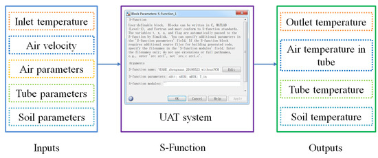
Figure 1.
The parameter calculation of system’s thermal performance through the MATLAB/SIMULINK platform using S-Function.
2.2. Model Assumptions
To simplify the dynamic performance prediction of the UAT system without sacrificing the prediction accuracy, some assumptions have been made, as follows:
- The soil is assumed to be homogeneous, and the thermophysical properties are considered isotropic.
- Air is incompressible with constant density and specific heat.
- The effect of air humidity variation on the heat-transfer process is ignored.
- The heat exchange along the vertical buried tube from the inlet to the buried depth is ignored.
- The thermal interference between two adjacent tubes is ignored.
- The heat conduction between the adjacent soil along the air flowing direction is ignored.
- The effect of convection and radiation on the ground surface on the heat-transfer process of the UAT system is ignored.
2.3. Mathematical Equations
In this system, the model of air, tube wall, and soil along the flowing air direction can be split into n volume elements and the distance between two-adjacent divided layers is denoted as Δx, as shown in Figure 2. The temperature of each layer is assumed to be the same as the discretized node. Each divided element follows the energy balance law. The energy balance equation of each volume element can be solved at each time step to iteratively calculate the temperature variation. In the mathematical model, the temperatures of each node at time t and the previous time are denoted as and . The linear mean temperature was adopted for the temperature between time t-dt and t [44]. Based on this, the nodal discretization of the air, tube, and soil located at the jth layer can be illustrated in Figure 3.
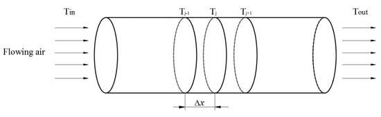
Figure 2.
The divided volume elements of the underground air tunnel system.
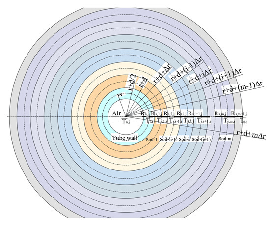
Figure 3.
Demonstration of the nodes for the air, tube wall, and soil layer.
(1) Air model:
From Equation (1):
where and are the air density and the specific heat capacity of air; is the divided air volume, , where is the tube inner radius and is the divided length; , , and are the mean air temperatures of the jth and (j-1)th layers and of the tube wall between times t and t-dt, respectively; is the air temperature at time t-dt; is the air flow rate, , where is the air velocity; and is the heat-transfer resistance between flowing air and tube wall:
where is the convective heat-transfer coefficient, , and n = 0.3 for cooling [32].
- is the area of the tube wall, .
- is the coefficient of heat conductivity of the tube wall.
- is the thickness of the tube wall.
- Re is the Reynolds number, .
- Pr is the Prandtl number, .
- is the air coefficient of heat conductivity. Re and Pr are Reynolds number and Prandtl. is the air dynamic viscosity.
(2) Tube wall model
From Equation (4), the temperature of node j at time t-dt is shown below:
where , , and are the tube density, specific heat capacity, and divided volume, respectively, and where .
- is the tube wall temperature at time t-dt.
- is the mean temperature of the 1st column soil between time t and t-dt.
- is the heat-transfer resistance between the tube wall and the 1st column soil.where is the heat conductivity of the soil. is the distance of the neighboring divided soil block radius.
(3) Soil model
1) For soil-1 model:
From Equation (7), the temperature of node j at time t-dt is shown below:
where and are the soil density and specific heat capacity, respectively.
- is the divided volume of the 1st column soil, .
- is the 1st column soil temperature at time t-dt.
- and are the mean temperatures of the 1st and 2nd column soils between times t and t-dt, respectively.
- is the heat-transfer resistance between the 1st column and the 2nd column soils:
2) For soil-i model:
From Equation (10):
is the ith column soil-divided volume at the jth layer.
.
is the temperature of the ith column soil at time t-dt.
, , and are the mean temperatures of the ith, (i-1)th, and (i+1)th column soils, respectively.
is the heat-transfer resistance between the (i-1)th and ith column soils.
is the heat-transfer resistance between the ith and (i+1)th column soils at the jth layer:
3) For the mth column soil:
From Equation (14):
is the divided volume of the mth column soil.
.
is the mth column soil temperature at time t-dt.
and are the mean temperatures of the mth and (m-1)th column soils between times t and t-dt, respectively.
is the outermost soil temperature, which can be obtained from experimental data.
is the heat-transfer resistance between the (m-1)th and the mth column soils:
is the heat-transfer resistance between the mth column and the outermost soil:
2.4. Overall System of Equations
Based on the abovementioned development of the mathematical model, each divided element or layer has equations. The total number of equations is . A matrix equation was thereafter developed as follows:
From Equation (18), the dynamic temperature was calculated by Equation (19).
The air, tube wall, and soil temperature for each divided element at time t can be calculated as follows:
where is the vector of the unknown mean temperature between times t and t-dt; is the corresponding matrix of coefficients, which are related to the air parameters, tube parameters, soil parameters, air velocity, etc.; and are the air temperature, tube wall temperature, and soil temperature values at times t-dt and t, respectively; and is the column vector of the known terms, e.g., inlet air temperature of and outermost soil temperature of .
2.5. Cooling Capacity Calculation
Based on the calculated air temperature, the cooling capacity of the UAT system at time t can be calculated by the following Equation (21) [45].
where and refer to the air mass flow rate and air specific heat in the tube. and refer to the inlet and outlet temperature at time t, respectively.
3. Model Validation
The prediction accuracy of the developed dynamic model was compared with the experimental results. The experimental platform of the UAT system was built in Changsha, China. The UAT system consisted of a power equipment and S-shaped buried tube with a depth of 3.5 m and a total length of 34 m. The tube was made of polyethylene (PE) with a diameter of 250 mm and wall thickness of 10 mm. The sensors are PT 100 thermocouple with a permissible error at ± 0.15 °C. All these sensors were calibrated using the ice-water mixture before being connected to the Agilent 34972A for the experimental testing. The airflow velocity in buried tube was measured using the vane probe type anemometer (TSI-9555) with an accuracy of ±3.0%. The schematic diagram of UAT system are presented in Figure 4. The input parameters used for the dynamic model validation are listed in Table 1.
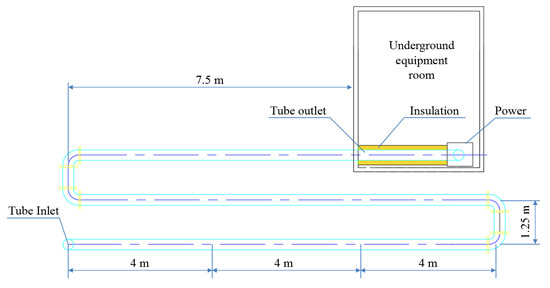
Figure 4.
Schematic diagram of underground air tunnel (UAT) system.

Table 1.
Input parameters for model validation.
The experimental validation was conducted for the cooling mode in summer. The experimental testing in summer was conducted from August 23rd to 24th, 2016, with a continuous operation for 24 h. The air velocity was 1 m/s during the experimental testing process.
Figure 5 shows the comparison results between the experimental testing and simulated results for outlet air temperature and cooling capacity in summer. As shown in Figure 5, the dynamic model-driven outlet temperature shows a similar trend to the monitored temperature from 15:30 to 7:30, whereas the dynamic model-driven outlet temperature shows a higher increasing trend than the experimental results. The temperature rise of the outlet air temperature is 0.61 °C for the experimental results, and the temperature rise is 1.43 °C for the simulated results. The underlying mechanism is due to the testing errors, resulting from the PT 100 thermocouple and the vane probe type anemometer. Furthermore, the maximum temperature difference between the monitored and simulated air temperature at the outlet is less than 0.81 °C. The corresponding average temperature difference is less than 0.13 °C. Furthermore, the maximum absolute relative deviation (MARE, as shown in Equation (22) [47]) between the monitored and simulated results for the air temperature at the outlet is approximately 3.18%.
where is the number of selected data samples, , and where and are the simulated and monitored air temperatures, respectively.
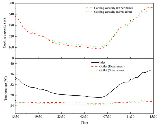
Figure 5.
The comparison between experiment and simulation data for outlet air temperature and cooling capacity.
Based on Equation (21), the maximum cooling capacity between the monitored and simulated results can be calculated as 39.59 W and the corresponding average cooling capacity difference is 8.90 W. Furthermore, the maximum absolute relative deviation between the monitored and simulated results for the cooling capacity can be calculated as 6.03%. According to the above comparison results, the developed dynamic model is accurate to further investigate the dynamic thermal performance for multidimensional parameter analysis.
4. Thermal Performance Analysis
In this section, the multidimensional parameter analysis has been conducted on geometrical parameters and operating parameters of the UAT system. Based on the developed dynamic model, the outlet temperature and cooling capacity of UAT system were predicted with respect to different tube lengths, tube thermal conductivities, tube diameters, and air velocities.
4.1. Effect of Tube Lengths
The effect of the tube length on the outlet temperature and cooling capacity was investigated, with the air velocity at 1 m/s and tube inner diameter at 250 mm. Other variables, e.g., inlet air temperatures, tube conductivities, and soil parameters, are kept constant.
Figure 6 shows the impacts of the tube lengths on the cooling capacity and outlet temperature. The average outlet temperatures and cooling capacities are presented in Table 2. As shown in Figure 6 and Table 2, when the tube length is 10 m, the UAT system shows the highest outlet temperature at 28.15 °C and the lowest cooling capacity at 163.29 W. With respect to the increase of the tube length from 10 to 60 m, the outlet temperature decreases from 28.15 °C to 24.40 °C and the cooling capacity increases from 163.29 to 401.95 W. The underlying mechanism is that a longer tube length can enhance the heat exchange between the flowing air and surrounding soil due to the increased time-duration of flowing air in the tube. However, as shown in Figure 6, with the increase of the tube length, the decreasing magnitude of the outlet temperature and the increasing magnitude of the cooling capacity decrease. For instance, when the tube length increases from 10 to 20 m, the decreasing magnitude of the outlet temperature is 1.57 °C and the increasing magnitude of the cooling capacity is 100.15 W. However, when the tube length increases from 50 to 60 m, the decreasing magnitude of the outlet temperature is only 0.23 °C and the increasing magnitude of the cooling capacity is 14.83 W. The underlying mechanism is that, as the decreasing magnitude of the soil temperature decreases with the increase of the tube length, the temperature difference between the flowing air and surrounding soil temperature will be saturated. By contrast, from the perspective of the initial economic investment, the increase of the buried tube length will significantly increase the initial, operational, and maintenance costs due to the difficulties in the system installation and operation processes. Therefore, when systematically considering the outlet temperature, the cooling capacity, and economic performance, the solution for the increase of the buried tube length is not techno-economically competitive, especially with the increase of the buried tube length.
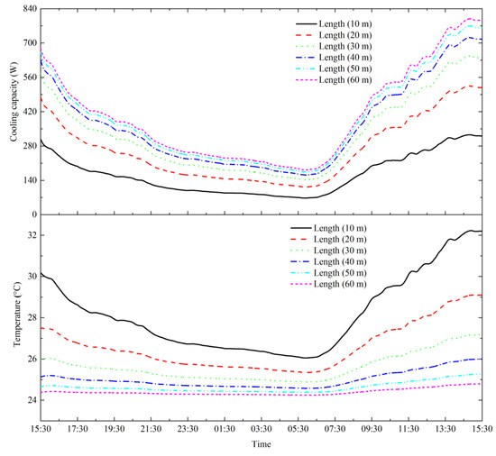
Figure 6.
The effect of different tube lengths on the cooling capacity and the outlet temperature.
Table 2.
The average outlet temperatures and cooling capacities.
4.2. Effect of Tube Thermal Conductivities
The effect of different tube conductivities on outlet temperature and cooling capacity is investigated, when the air velocity, tube length, and tube diameter are set at 1 m/s, 32 m, and 250 mm, respectively. Other variables, e.g., inlet air temperatures and soil parameters, are kept constant.
Figure 7 shows the impacts of tube conductivities on the outlet temperature and cooling capacity. The average outlet temperatures and cooling capacities are listed in Table 3. As shown in Figure 7 and Table 3, the increase of tube conductivities can decrease the outlet temperature and can increase the cooling capacity. For instance, with the increase of the tube coefficient of heat conductivity from 0.5 to 16 W/(m K), the average outlet temperature decreases from 25.30 °C to 25.16 °C and the average cooling capacity increases from 344.43 W to 353.62 W. Furthermore, with the increase of coefficient of heat conductivity of the tube, the decreasing magnitude of the outlet temperature and the increasing magnitude of the cooling capacity decrease. For instance, with the increase of the coefficient of heat conductivity of the tube from 0.5 to 1 W/(m K), the decreasing magnitude of the outlet temperature is 0.07 °C (from 25.30 °C to 25.23 °C), and the increasing magnitude of the average cooling capacity is 4.71 W (from 344.43 to 349.14 W). With the increase of the coefficient of heat conductivity of the tube from 1 to 16 W/(m K), the decreasing magnitude of the outlet temperature is 0.07 °C (from 25.23 °C to 25.16 °C), and the increasing magnitude of the average cooling capacity is 4.48 W (from 349.14 to 353.62 W). In can be concluded that both the outlet temperature and average cooling capacity are less dependent on the coefficient of heat conductivity of tube materials. Therefore, the solution for the increase of the coefficient of heat conductivity of tubes is not quite techno-economically competitive for the performance enhancement.
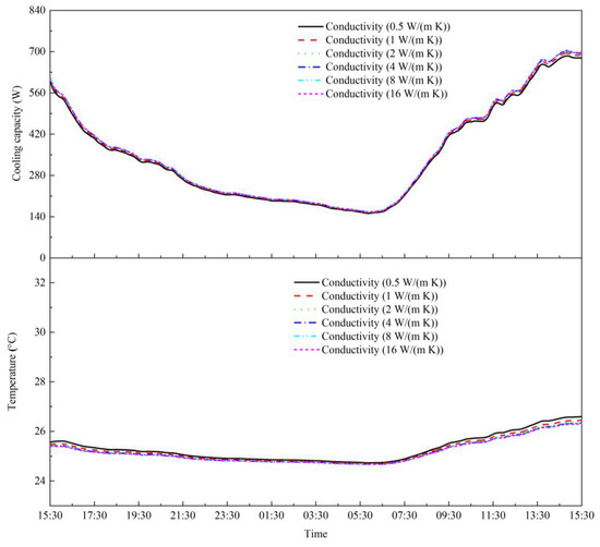
Figure 7.
The effect of different tube conductivities on the outlet temperature and cooling capacity.
Table 3.
The average outlet temperatures and cooling capacities.
4.3. Effect of Tube Diameters
The effect of different tube diameters on the outlet temperature and the cooling capacity is investigated in the scenario when the air velocity and tube length are 1 m/s and 32 m, respectively. In this study, the selected maximum tube diameter is 400 mm considering the assumption of thermal interference between the adjoining tubes in Section 2.2. As reported in Reference [48], a distance of more than 2D (D is the tube diameter) between the adjoining tubes enables the absolute mean differential of the ratio of the annual exchanged heat rate to be less than 2.1%. Other variables, e.g., inlet air temperatures, tube conductivities, and soil parameters, are kept constant.
Figure 8 shows the impacts of tube diameters on the cooling capacity and the outlet temperature. The average outlet temperatures and cooling capacities are presented in Table 4. As shown in Figure 8 and Table 4, the outlet temperature and cooling capacity of the UAT system increase with the increase of the tube diameter. Specifically, with the tube diameter increasing from 100 to 400 mm, the average outlet temperature increases from 24.05 °C to 26.67 °C and the average cooling capacity increases from 67.84 to 659.29 W. Furthermore, a larger tube diameter is more conducive to improving the cooling capacity. For instance, the increasing magnitude of the average cooling capacity is 78.24 W (from 67.84 to 146.08 W) when the tube diameter increases from 100 to 150 mm and the increasing magnitude of the average cooling capacity is 105.51 W (from 553.78 to 659.29 W) when the tube diameter increases from 350 to 400 mm. However, it is noteworthy that a larger tube diameter will result in a higher outlet temperature, resulting in the increase of the space cooling load for indoor thermal environment. For instance, the maximum outlet temperature can reach 28.96 °C when the tube diameter is 400 mm, and thus, a high temperature has difficulty satisfying the requirements of indoor thermal comfort. In addition, a larger tube diameter will also result in a higher system’s initial investment. Thus, an appropriate tube diameter should be carefully selected based on the balance between the outlet temperature and cooling capacity in practical application.
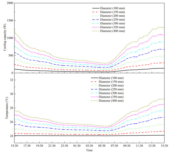
Figure 8.
Evolution of outlet temperature and cooling capacity with respect to tube diameters.
Table 4.
The average outlet temperatures and cooling capacities.
4.4. Effect of Air Velocities
The effect of different air velocities on the outlet air temperature and cooling capacity is investigated in the scenario when the tube length is 32 m and the tube diameter is 250 mm. Other variables, e.g., inlet air temperature, tube parameters, and soil parameters, are kept constant.
Figure 9 shows impacts of air velocities on the outlet temperature and cooling capacity. The average outlet temperatures and cooling capacities are presented in Table 5. As shown in Figure 9 and Table 5, both the outlet temperature and cooling capacity increase with the increase of the air velocity. To be specific, with the increase of the air velocity from 0.5 to 4 m/s, the average outlet temperature increases from 24.82 °C to 27.05 °C and the cooling capacity increases from 187.50 to 931.96 W, respectively. The main reason is that a larger air velocity leads to less time-duration for the heat exchange between the surrounding soil and the flowing air. Figure 9 also shows that the outlet air temperature is more stable and lower with the decrease of air velocity. However, the smaller air velocity will lead to a lower cooling capacity. Thus, the trade-off between the lower outlet temperature and larger cooling capacity has to be made for practical applications.
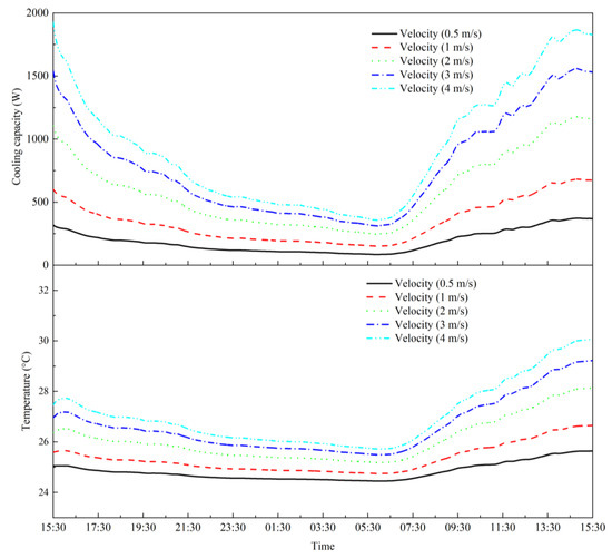
Figure 9.
The effect of different air velocities on the outlet temperature and cooling capacity.
Table 5.
The average outlet temperatures and cooling capacities.
5. Conclusions and Future Studies
In this study, an underground air tunnel (UAT) system was proposed for the utilisation of geothermal energy for space cooling of buildings. A dynamic mathematical model of the underground air tunnel system was developed on the MATLAB/SIMULINK platform for the dynamic performance prediction, together with an on-site experimental test-rig for the validation. Compared to conventional UAT model developed on the CFD platform, the developed dynamic model on the MATLAB/SIMULINK platform is more flexible for the multi-domain simulation with higher flexibility for the multidimensional parametrical analysis. Based on the developed dynamic model, the multidimensional parametrical analysis has been conducted on geometrical parameters (i.e., tube lengths, tube diameters, and tube thermal conductivities) and operating parameters (i.e., air velocities) to provide technical guidance for the optimal design and robust operation. The main results of this study can be summarized as follows:
- The on-site experimental validation indicates that the proposed mathematical model is accurate for the dynamic performance prediction. Compared with the on-site experimental data, the developed model is credible and accurate with a maximum absolute relative deviation of 3.18% and 6.03% for outlet air temperature and cooling capacity, respectively
- The comprehensive and systematic parametrical analysis results indicated that, with the increase of the tube length, the outlet temperature decreases and the cooling capacity increases significantly whereas the decreasing magnitude of outlet temperature and the increasing magnitude of cooling capacity reduce
- The system performance is slightly dependent on the tube materials, and the technical solution, e.g., the increase of the coefficient of heat conductivity of the tube, is not efficient to improve the system performance
- Both outlet temperature and cooling capacity of the UAT system increase with the increase of tube diameter and air velocity. The increase of tube diameter and air velocity can improve the system’s cooling capacity. However, the decrease of tube diameter and air velocity will result in a more stable and lower outlet temperature, which can reduce the cooling load for indoor thermal comfort
The above conclusions are drawn under a 24-h continuous operation. However, the outlet air temperature and cooling capacity of the UAT system are dependent on the operation time due to the gradual heating of the soil around the buried tubes. Therefore, the assessment of the cooling potential should be carried out over a long-time operation period, e.g., several months, in our following-up study. Further studies need to be conducted for the trade-offs between tube diameter and air velocity for the bi-criteria performance enhancement between cooling capacity and outlet temperature. Furthermore, multivariable optimizations [49] with multi-criteria performances, such as cooling capacity, coefficient of performance (COP), and economic performance and system efficiency, will be conducted in our following-up study. In addition, geometrical configurations of phase change material systems (e.g., displacement position of PCM outside and inside the tube or PCM in the surrounding soil) will be experimentally investigated for technical performance enhancement.
Author Contributions
Conception of the study and development of the methodology, L.T.; computer model development, simulation, and data analyses, Z.L.; supervision of the whole work Y.Z. and G.Z.; writing, L.T., Z.L., and D.Q. All authors have read and agreed to the published version of the manuscript.
Funding
This research work was funded by the China Construction Fifth Engineering Division Corp., Ltd. (NO. 900201528). This research is supported by the Hong Kong Polytechnic University. The authors also thank the editors and an anonymous reviewer for their useful comments and suggestions.
Conflicts of Interest
The authors declare no conflict of interest.
Nomenclature
| Symbols |
| Specific heat capacity (J/(kg °C)) |
| Tube wall thickness (m) |
| Divided length (m) |
| Heat-transfer coefficient (W/(m2·°C)) |
| Mass flow rate (kg/s) |
| Prandtl number Q: Cooling capacity (W) |
| Reynolds number |
| Thermal resistance between different units (°C/W) |
| Tube inner radius (m) |
| Distance of neighboring divided soil block radius (m) |
| Heat-transfer area (m2) Temperature at time t (°C) |
| Temperature at time t-dt (°C) |
| Average temperature between times t and t-dt (°C) |
| Volume of divided unit (m3) |
| V: Air velocity |
| Δx: Distance between two-adjacent divided layers |
| Greek letters |
| Density (m3/kg) |
| Thermal conductivity (W/(m·°C)) |
| Dynamic viscosity of air |
| Subscripts |
| a: Air layer |
| Outermost soil layer |
| Radial direction Position of the divided soil |
| in: Tube inlet |
| Vertical direction position of the divided unit |
| k: The number of selected data samples |
| m: The mth column of the divided soil layer |
| out: Tube outlet |
| s: Soil layer |
| t: Tube layer |
| Abbreviations |
| ASHE: Air–soil heat exchanger |
| CFD: Computational fluid dynamic |
| EAT: Earth–air tunnel |
| EAHE: Earth-to-air heat exchanger |
| HVAC: Heating ventilation and air conditioning |
| MARD: Maximum absolute relative deviation |
| UAT: Underground air tunnel |
References
- Liu, Z.; Yu, Z.; Yang, T.; Qin, D.; Li, S.; Zhang, G.; Haghighat, F.; Joybari, M.M. A review on macro-encapsulated phase change material for building envelope applications. Build. Environ. 2018, 144, 281–294. [Google Scholar] [CrossRef]
- Zeng, C.; Yuan, Y.; Xiang, B.; Cao, X.; Zhang, Z.; Sun, L. Thermal and infrared camouflage performance of earth-air heat exchanger for cooling an underground diesel generator room for protective engineering. Sustain. Cities Soc. 2019, 47, 101437. [Google Scholar] [CrossRef]
- Zhou, Y.; Zheng, S.; Zhang, G. Artificial neural network based multivariable optimization of a hybrid system integrated with phase change materials, active cooling and hybrid ventilations. Energy Convers. Manag. 2019, 197, 111859. [Google Scholar] [CrossRef]
- Zhou, Y.; Zheng, S.; Zhang, G. Machine learning-based optimal design of a phase change material integrated renewable system with on-site PV, radiative cooling and hybrid ventilations—Study of modelling and application in five climatic regions. Energy 2020, 192, 116608. [Google Scholar] [CrossRef]
- Zhou, Y.; Cao, S.; Hensen, J.L.M.; Lund, P.D. Energy integration and interaction between buildings and vehicles: A state-of-the-art review. Renew. Sustain. Energy Rev. 2019, 114, 109337. [Google Scholar] [CrossRef]
- Zhou, Y.; Zheng, S.; Zhang, G. Machine-learning based study on the on-site renewable electrical performance of an optimal hybrid PCMs integrated renewable system with high-level parameters’ uncertainties. Renew. Energy 2020. [Google Scholar] [CrossRef]
- Tang, L.; Zhou, Y.; Zheng, S.; Zhang, G. Exergy-based optimisation of a phase change materials integrated hybrid renewable system for active cooling applications using supervised machine learning method. Sol. Energy 2020, 195, 514–526. [Google Scholar] [CrossRef]
- Zhou, Y.; Zheng, S.; Zhang, G. Study on the energy performance enhancement of a new PCMs integrated hybrid system with the active cooling and hybrid ventilations. Energy 2019, 179, 111–128. [Google Scholar] [CrossRef]
- Zhou, Y.; Yu, C.W.F.; Zhang, G. Study on heat-transfer mechanism of wallboards containing active phase change material and parameter optimisation with ventilation. Appl. Therm. Eng. 2018, 144, 1091–1108. [Google Scholar] [CrossRef]
- Liu, Z.; Sun, P.; Li, S.; Yu, Z.; El Mankibi, M.; Roccamena, L.; Yang, T.; Zhang, G. Enhancing a vertical earth-to-air heat exchanger system using tubular phase change material. J. Clean. Prod. 2019, 237, 117763. [Google Scholar] [CrossRef]
- Yang, D.; Wei, H.; Shi, R.; Wang, J. A demand-oriented approach for integrating earth-to-air heat exchangers into buildings for achieving year-round indoor thermal comfort. Energy Convers. Manag. 2019, 182, 95–107. [Google Scholar] [CrossRef]
- Zhou, Y.; Zheng, S.; Zhang, G. Multivariable optimisation of a new PCMs integrated hybrid renewable system with active cooling and hybrid ventilations. J. Build. Eng. 2019, 26, 100845. [Google Scholar] [CrossRef]
- Liu, X.; Zhou, Y.; Zhang, G. Numerical study on cooling performance of a ventilated Trombe wall with phase change materials. Build. Simul. 2018, 11, 1–18. [Google Scholar] [CrossRef]
- Zhou, Y.; Yu, C.W. The year-round thermal performance of a new ventilated Trombe wall integrated with phase change materials in the hot summer and cold winter region of China. Indoor Built Environ. 2018, 28, 195–216. [Google Scholar] [CrossRef]
- Zhou, Y.; Zheng, S.; Chen, H.; Zhang, G. Thermal performance and optimized thickness of active shape-stabilized PCM boards for side-wall cooling and under-floor heating system. Indoor Built Environ. 2016, 25, 1279–1295. [Google Scholar] [CrossRef]
- Liu, X.; Zhou, Y.; Li, C.-Q.; Lin, Y.; Yang, W.; Zhang, G. Optimization of a new phase change material integrated photovoltaic/thermal panel with the active cooling technique using taguchi method. Energies 2019, 12, 1022. [Google Scholar] [CrossRef]
- Zhou, Y.; Liu, X.; Zhang, G. Performance of buildings integrated with a photovoltaic–thermal collector and phase change materials. Procedia Eng. 2017, 205, 1337–1343. [Google Scholar] [CrossRef]
- Liu, Z.; Yu, Z.; Yang, T.; El Mankibi, M.; Roccamena, L.; Sun, Y.; Sun, P.; Li, S.; Zhang, G. Experimental and numerical study of a vertical earth-to-air heat exchanger system integrated with annular phase change material. Energy Convers. Manag. 2019, 186, 433–449. [Google Scholar] [CrossRef]
- Liu, Z.; Yu, Z.; Yang, T.; Roccamena, L.; Sun, P.; Li, S.; Zhang, G.; El Mankibi, M. Numerical modeling and parametric study of a vertical earth-to-air heat exchanger system. Energy 2019, 172, 220–231. [Google Scholar] [CrossRef]
- Zeng, R.; Li, H.; Jiang, R.; Liu, L.; Zhang, G. A novel multi-objective optimization method for CCHP–GSHP coupling systems. Energy Build. 2016, 112, 149–158. [Google Scholar] [CrossRef]
- Liu, Z.; Yu, Z.; Yang, T.; Li, S.; El Mankibi, M.; Roccamena, L.; Qin, D.; Zhang, G. Experimental investigation of a vertical earth-to-air heat exchanger system. Energy Convers. Manag. 2019, 183, 241–251. [Google Scholar] [CrossRef]
- Zeng, R.; Zhang, X.; Deng, Y.; Li, H.; Zhang, G. An off-design model to optimize CCHP-GSHP system considering carbon tax. Energy Convers. Manag. 2019, 189, 105–117. [Google Scholar] [CrossRef]
- Liu, J.; Yu, Z.; Liu, Z.; Qin, D.; Zhou, J.; Zhang, G. Performance Analysis of Earth-air Heat Exchangers in Hot Summer and Cold Winter Areas. Procedia Eng. 2017, 205, 1672–1677. [Google Scholar] [CrossRef]
- Wei, H.; Yang, D. Performance evaluation of flat rectangular earth-to-air heat exchangers in harmonically fluctuating thermal environments. Appl. Therm. Eng. 2019, 162, 114262. [Google Scholar] [CrossRef]
- Liu, Z.; Yu, Z.; Yang, T.; Li, S.; Mankibi, M.E.; Roccamena, L.; Qin, D.; Zhang, G. Designing and evaluating a new earth-to-air heat exchanger system in hot summer and cold winter areas. Energy Procedia 2019, 158, 6087–6092. [Google Scholar] [CrossRef]
- Bordoloi, N.; Sharma, A.; Nautiyal, H.; Goel, V. An intense review on the latest advancements of Earth Air Heat Exchangers. Renew. Sustain. Energy Rev. 2018, 89, 261–280. [Google Scholar] [CrossRef]
- Agrawal, K.K.; Misra, R.; Agrawal, G.D.; Bhardwaj, M.; Jamuwa, D.K. The state of art on the applications, technology integration, and latest research trends of earth-air-heat exchanger system. Geothermics 2019, 82, 34–50. [Google Scholar] [CrossRef]
- Zhou, Y.; Zheng, S. Machine learning-based multi-objective optimisation of an aerogel glazing system using NSGA-II—Study of modelling and application in the subtropical climate Hong Kong. J. Clean. Prod. 2020. [Google Scholar] [CrossRef]
- Zhou, Y.; Zheng, S. Uncertainty study on thermal and energy performances of a deterministic parameters based optimal aerogel glazing system using machine-learning method. Energy 2020. [Google Scholar] [CrossRef]
- Bisoniya, T.S.; Kumar, A.; Baredar, P. Experimental and analytical studies of earth–air heat exchanger (EAHE) systems in India: A review. Renew. Sustain. Energy Rev. 2013, 19, 238–246. [Google Scholar] [CrossRef]
- Agrawal, K.K.; Agrawal, G.D.; Misra, R.; Bhardwaj, M.; Jamuwa, D.K. A review on effect of geometrical, flow and soil properties on the performance of Earth air tunnel heat exchanger. Energy Build. 2018, 176, 120–138. [Google Scholar] [CrossRef]
- Niu, F.; Yu, Y.; Yu, D.; Li, H. Heat and mass transfer performance analysis and cooling capacity prediction of earth to air heat exchanger. Appl. Energy 2015, 137, 211–221. [Google Scholar] [CrossRef]
- Fazlikhani, F.; Goudarzi, H.; Solgi, E. Numerical analysis of the efficiency of earth to air heat exchange systems in cold and hot-arid climates. Energy Convers. Manag. 2017, 148, 78–89. [Google Scholar] [CrossRef]
- Mathur, A.; Surana, A.K.; Verma, P.; Mathur, S.; Agrawal, G.D.; Mathur, J. Investigation of soil thermal saturation and recovery under intermittent and continuous operation of EATHE. Energy Build. 2015, 109, 291–303. [Google Scholar] [CrossRef]
- Yang, D.; Zhang, J. Analysis and experiments on the periodically fluctuating air temperature in a building with earth-air tube ventilation. Build. Environ. 2015, 85, 29–39. [Google Scholar] [CrossRef]
- Wei, H.; Yang, D.; Guo, Y.; Chen, M. Coupling of earth-to-air heat exchangers and buoyancy for energy-efficient ventilation of buildings considering dynamic thermal behavior and cooling/heating capacity. Energy 2018, 147, 587–602. [Google Scholar] [CrossRef]
- Misra, R.; Bansal, V.; Agrawal, G.D.; Mathur, J.; Aseri, T.K. CFD analysis based parametric study of derating factor for Earth Air Tunnel Heat Exchanger. Appl. Energy 2013, 103, 266–277. [Google Scholar] [CrossRef]
- Aslam Bhutta, M.M.; Hayat, N.; Bashir, M.H.; Khan, A.R.; Ahmad, K.N.; Khan, S. CFD applications in various heat exchangers design: A review. Appl. Therm. Eng. 2012, 32, 1–12. [Google Scholar] [CrossRef]
- Azzolin, M.; Mariani, A.; Moro, L.; Tolotto, A.; Toninelli, P.; Del Col, D. Mathematical model of a thermosyphon integrated storage solar collector. Renew. Energy 2018, 128, 400–415. [Google Scholar] [CrossRef]
- El Mankibi, M.; Zhai, Z.; Al-Saadi, S.N.; Zoubir, A. Numerical modeling of thermal behaviors of active multi-layer living wall. Energy Build. 2015, 106, 96–110. [Google Scholar] [CrossRef]
- Chen, Y.; Treado, S. Development of a simulation platform based on dynamic models for HVAC control analysis. Energy Build. 2014, 68, 376–386. [Google Scholar] [CrossRef]
- De Rosa, M.; Bianco, V.; Scarpa, F.; Tagliafico, L.A. Heating and cooling building energy demand evaluation; a simplified model and a modified degree days approach. Appl. Energy 2014, 128, 217–229. [Google Scholar] [CrossRef]
- Kıyan, M.; Bingöl, E.; Melikoğlu, M.; Albostan, A. Modelling and simulation of a hybrid solar heating system for greenhouse applications using Matlab/Simulink. Energy Convers. Manag. 2013, 72, 147–155. [Google Scholar] [CrossRef]
- Stathopoulos, N.; El Mankibi, M.; Issoglio, R.; Michel, P.; Haghighat, F. Air–PCM heat exchanger for peak load management: Experimental and simulation. Sol. Energy 2016, 132, 453–466. [Google Scholar] [CrossRef]
- Bisoniya, T.S.; Kumar, A.; Baredar, P. Energy metrics of earth–air heat exchanger system for hot and dry climatic conditions of India. Energy Build. 2015, 86, 214–221. [Google Scholar] [CrossRef]
- Ghosal, M.K.; Tiwari, G.N. Modeling and parametric studies for thermal performance of an earth to air heat exchanger integrated with a greenhouse. Energy Convers. Manag. 2006, 47, 1779–1798. [Google Scholar] [CrossRef]
- Zhang, L.; Zhang, Q.; Huang, G. A transient quasi-3D entire time scale line source model for the fluid and ground temperature prediction of vertical ground heat exchangers (GHEs). Appl. Energy 2016, 170, 65–75. [Google Scholar] [CrossRef]
- Yoon, G.; Tanaka, H.; Okumiya, M. Study on the design procedure for a multi-cool/heat tube system. Sol. Energy 2009, 83, 1415–1424. [Google Scholar] [CrossRef]
- Zhou, Y.; Zheng, S.; Zhang, G. A review on cooling performance enhancement for phase change materials integrated systems—flexible design and smart control with machine learning applications. Build. Environ. 2020, 10, 6786. [Google Scholar] [CrossRef]


© 2020 by the authors. Licensee MDPI, Basel, Switzerland. This article is an open access article distributed under the terms and conditions of the Creative Commons Attribution (CC BY) license (http://creativecommons.org/licenses/by/4.0/).