A Benders’ Decomposition Approach for Renewable Generation Investment in Distribution Systems

Abstract

A model suitable to obtain where and when renewable energy sources (RES) should be allocated as part of generation planning in distribution systems is formulated. The proposed model starts from an existing two-stage stochastic mixed-integer linear programming (MILP) problem including investment and scenario-dependent operation decisions. The aim is to minimize photovoltaic and wind investment costs, operation costs, as well as total substation costs including the cost of the energy bought from substations and energy losses. A new Benders’ decomposition framework is used to decouple the problem between investment and operation decisions, where the latter can be further decomposed into a set of smaller problems per scenario and planning period. The model is applied to a 34-bus system and a comparison with a MILP model is presented to show the advantages of the model proposed.

1. Introduction

Distributed generation (DG) has been used to produce energy in remote and isolated places, where the distance between the demand and the producer is short [1]. At present, this trend is changing as it has been proven that DG provides technical, economic, and environmental improvements [2]. The benefits of using DG are based on the reduction of network losses, the voltage level improvement, or the dependence reduction of energy, fuel prices, and traditional generation. All these advantages cause CO2 emission reduction [3,4]. On the other hand, DG has also disadvantages, mainly related to technical aspects due to the fact that the existing networks have not been designed to incorporate this type of generation [2]. Some drawbacks are reverse current flows, the need for network redesign, or frequency instability [5].

In addition, planning of distribution networks must account for renewable generation uncertainty to meet the future demand in any possible future scenario. In that case, the decisions to be made could be to invest in the network, in substations, in DG generation, or in any combination of them [6]. When the chosen option is DG, it is necessary to determine the type of location, by solving the Distribution Generation Planning (DGP) problem. An example of this sort of problems can be seen in [7], where a linear model that optimizes size and location of DG is used. The objective function maximizes DG real power. In [6], a model is proposed for minimizing the investment and operation DG costs, the cost of the electricity bought from the substation, and the cost of network losses of a distribution company. The model is formulated as a mixed-integer-nonlinear one. Other authors have worked with particle swarm optimization methods [8], where a multi-objective model considers investment and operating costs of new generation, the cost of the energy purchased, and CO2 emission cost.

A number of references using Benders’ decomposition to solve computational-complex problems in distribution [9,10,11,12] and transmission systems [13,14,15,16,17] can be found in the technical literature.

The DGP is addressed by a multi-objective mixed-integer linear problem in [9], using Benders’ decomposition with an implicit enumeration algorithm where cost and reliability, among others, are included in the objectives’ set. No renewable technology is modeled, just feeders and substations. Another multi-objective operation approach is developed in [10]. In this case, the aim is to minimize the total operational costs and emissions, as well as to generate Pareto-optimal solutions for the energy and reserve scheduling problem, using fuzzy decision-making processes. The scenario combination merges wind generation and forecasted demand. The problem is formulated as mixed-integer non-linear problem. Reference [11] studies the point of view of a local distribution company to maximize its profit, using nodal hourly prices within a smart grid. DG, including fossil fuel and renewable units, is taken into account. Reference [12] deals with the day-ahead unit commitment problem in a microgrid system. The problem is formulated as a stochastic mixed integer program that takes into account the uncertainty in PV generation.

A generation expansion planning model is proposed in [13] where the network is disregarded. It includes a generic model for renewable units (wind and solar) and hydro units modeled as storage units. Another generation expansion planning in generalized networks is studied in [14] considering production costs and system reliability in the lower level and the expansion plan in the upper level. A transmission expansion planning model is proposed in [15] incorporating the uncertainty of wind units via scenarios, including the cost of the added lines, and wind curtailment and using a DC power flow. Studies [16,17] propose complementarity models to determine the optimal investment decisions of a profit-oriented private investor interested in building new conventional and wind-power generating units, respectively.

The basis of this paper is a two-stage stochastic mixed-integer linear programming problem (MILP) that is used to determine where and when renewable energy sources should be allocated as part of generation planning in distribution systems [18]. The model proposed in [18] has an important limitation; namely, its computational burden is very high if a large number of scenarios and planning periods is considered. In the worst case, the problem may be even intractable.

Despite this relevant issue, the problem described in [18] has an interesting property: if investment variables are fixed, the problem can be decomposed per scenario and planning period. The proposed Benders’ decomposition algorithm takes advantage of this decomposable problem structure to reduce the computational burden of the problem. This is the main benefit of the proposed approach.

Note that, to the best of our knowledge, there is no reference in the technical literature that considers a Benders’ decomposition approach for a stochastic multi-stage DGP problem such as the one considered in this paper. The existing literature has not taken into account the benefits of Benders’ decomposition for solve the DGP problem with a large number of scenarios of renewable energy. This problem is generally intractable for realistic case studies since it is necessary to consider a large number of scenarios and time periods to obtain informed expansion decisions. Moreover, it includes binary variables that further complicate the problem. Therefore, the traditional resolution methods, as a MILP, for stochastic multi-stage DGP problems are not viable. The Benders’ decomposition model presented, although it has greater computational complexity, dramatically reduces resolution times. This model can solve problems with a large number of scenarios and planning periods. In addition, it is able to solve problems that are typically intractable with traditional methods.

Given the above, the contributions of this work are:

• The stochastic multi-stage DGP problem is formulated using Benders’ decomposition that decomposes the problem per both scenario and planning period and
• A comparison with a standard MILP model is provided and results with a 34-bus test case are shown, where the significant computational advantage of using Benders’ decomposition with respect to the MILP model is also shown.

2. Notation

Subscripts t, k, and ω below refer to the values in year t, time block k, and scenario ω, respectively. Superindex $\left(\mathsf{\upsilon }\right)$ indicates the values in the $\mathsf{\upsilon }$-th Benders’ iteration. All indices, sets, constants, parameters and variables used in the document are shown in Table 1.

Table 1. Notation.

Indices and Sets
${\Omega }^K$	Set of indices of time blocks.
${\Omega }^L$	Set of indices of load buses.
${\Omega }^N$	Set of indices of branches.
${\Omega }^R$	Set of indices of blocks used in the piecewise linearization.
${\Omega }^{SS}$	Set of indices of substation buses.
${\Omega }^T$	Set of indices of years.
${\Psi }_k^{\omega }$	Set of indices of scenarios for the k-th block.
k	Index of time blocks.
n, m	Indices of buses.
r	Index used in the linearization.
t	Index of years.
ω	Index of scenarios.
Constants and Parameters
$c{a}^{pv}$	PV module annualized investment cost [$€$].
$c{a}^{wd}$	Wind turbine annualized investment cost [$€$].
$c{a}^{SS}$	Transformer annualized investment cost [$€$].
$c{i}^{pv}$	PV module investment cost [$€$].
$c{i}^{wd}$	Wind turbine investment cost [$€$].
$c{i}^{SS}$	Transformer investment cost [€].
$c{i}^{bgt}$	Investment budget per year [€].
$c{i}_{LC}^{bgt}$	Investment budget throughout the life cycle of the new devices [€].
${\mathit{com}}^{pv}$	PV module operation and maintenance costs [$€/\mathrm{MWh}$].
${\mathit{com}}^{wd}$	Wind turbine operation and maintenance costs [$€/\mathrm{MWh}$].
$c^{loss}$	Loss cost [$€/\mathrm{MWh}$].
cns	Cost of energy not supplied [$€/\mathrm{MWh}$].
Cpv,n	Vector of candidate buses $n$ to install PV modules.
$c_{k,\omega }^{SS}$	Cost of the energy purchased by the substation [$€/\mathrm{MWh}$].
$C^{wd,n}$	Vector of candidate buses $n$ to install wind turbines.
$d$	Discount rate.
$f_t$	Increasing load factor.
$f_{k,\omega }^{ld}$	Demand factor.
$f_t^{SS}$	Increasing energy cost factor.
$f_{k,\omega }^{wd}$	Wind turbine power factor available.
$f_{k,\omega }^{pv}$	PV module power factor available.
$\overline{I^{n,m}}$	Maximum current through branch $n,m$ [${\mathrm{A}}_{pu}$].
$i_{ }$	Interest rate.
$L{C}^{SS}$	Transformer life cycle [$\mathrm{years}$].
$L{C}^{pv}$	PV module life cycle [$\mathrm{years}$].
$L{C}^{wd}$	Wind turbine life cycle [$\mathrm{years}$].
$m_{t,k,\omega }^{n,m,r}$	Slope of the r-th block of the piecewise linearization for branch $n,m$.
$N_k^h$	Number of hours in time block $k$ [$\mathrm{hours}$].
$P^{ld,n}$	Active power load in bus $n$ [${\mathrm{MW}}_{pu}$].
$\overline{P^{pv}}$	Maximum active power output of PV modules [${\mathrm{MW}}_{pu}$].
$\overline{P^{wd}}$	Maximum active power output of wind turbine [${\mathrm{MW}}_{pu}$].
$\overline{P^{node}}$	Maximum active power that can be installed in each bus [${\mathrm{MW}}_{pu}$].
$Q^{ld,n}$	Reactive power load in bus $n$ [${\mathrm{MVar}}_{pu}$].
$R^{n,m}$	Resistance of branch $n,m$ [${\mathsf{\Omega }}_{\mathrm{pu}}$].
$\overline{R}$	Number of blocks used in the piecewise linearization.
$\overline{S^{SS}}$	Maximum power output of new transformers [${\mathrm{MVA}}_{pu}$].
$\overline{S^{NEW,n}}$	Maximum new power allowed for installment in the substation in bus $n$ [${\mathrm{MVA}}_{pu}$].
$S^{SS,n}$	Existing power in the substation in bus $n$ [${\mathrm{MVA}}_{pu}$].
$S^{base}$	Power base [$\mathrm{MVA}$].
$tan\left({\phi }^{SS}\right)$	Tangent angle in substation.
$tan\left({\phi }^{pv}\right)$	Tangent angle of PV modules.
$tan\left({\phi }^{wd}\right)$	Tangent angle of wind turbines.
$\underset{\_}{V}$	Minimum voltage magnitude [${\mathrm{kV}}_{pu}$].
$\overline{V}$	Maximum voltage magnitude [${\mathrm{kV}}_{pu}$].
$V^{nom}$	Nominal voltage of the distribution network [${\mathrm{kV}}_{pu}$].
$X^{n,m}$	Reactance of branch $n,m$ [${\mathsf{\Omega }}_{pu}$].
$\overline{Y^{pv,n}}$	Maximum number of PV modules to be installed in bus $n$.
$\overline{Y^{wd,n}}$	Maximum number of wind turbines to be installed in bus n.
Zn,m	Impedance of branch $n,m$ [${\mathsf{\Omega }}_{pu}$].
${\gamma }_{k,\omega }$	Weight of scenario $\omega$ in time block $k$.
$\mathsf{∆}{S}_{t,k,\omega }^{n,m,r}$	Upper bound of each r block of the power flow through branch $n,m$ [${\mathrm{MVA}}_{pu}$].
${\beta }_t$	Present worth factor.
Variables
$c{i}_t$	Investment cost [$€$].
$clos{s}_{t,k,\omega }$	Losses cost [$€/\mathrm{h}$].
$cn{s}_{t,k,\omega }$	Penalty for not supplied energy [$€/\mathrm{h}$].
$cne{w}_{t,k,\omega }$	Maintenance and operation costs of DG candidates [$€/h$].
$co{m}_{t,k,\omega }$	Maintenance and operation total costs [$€/\mathrm{h}$].
$cs{s}_{t,k,\omega }$	Cost of energy purchased by the substation [$€/\mathrm{h}$].
$I_{t,k,\omega }^{sqr,n,m}$	Square of current flow magnitude of branch n, m [$A_{pu}^2$].
$P{T}_t^{wd,n}$	Active power of wind turbines to be installed in bus $n$ [${\mathrm{MW}}_{pu}$].
$P{T}_t^{pv,n}$	Active power of PV modules to be installed in bus $n$ [${\mathrm{MW}}_{pu}$].
$P_{t,k,\omega }^{ns,n}$	Not supplied active power in bus $n$ [${\mathrm{MW}}_{pu}$].
$P_{t,k,\omega }^{pv,n}$	Active power injected by PV modules in bus $n$ [${\mathrm{MW}}_{pu}$].
$P_{t,k,\omega }^{wd,n}$	Active power injected by wind turbines in bus $n$ [${\mathrm{MW}}_{pu}$].
$P_{t,k,\omega }^{SS,n}$	Active power purchased by the substation in bus $n$ [${\mathrm{MW}}_{pu}$].
$P_{t,k,\omega }^{+,n,m}$	Active power flow in branch $n,m$ in the forward direction [${\mathrm{MW}}_{pu}$].
$P_{t,k,\omega }^{-,n,m}$	Active power flow in branch $n,m$ in the backward direction [${\mathrm{MW}}_{pu}$].
$Q_{t,k,\omega }^{ns,n}$	Not supplied reactive power in bus $n$ [${\mathrm{MVAr}}_{pu}$].
$Q_{n,t,k,\omega }^{pv,n}$	Reactive power injected by PV modules in bus $n$ [${\mathrm{MVAr}}_{pu}$].
$Q_{t,k,\omega }^{wd,n}$	Reactive power injected by wind turbines in bus [${\mathrm{MVAr}}_{pu}$].
$Q_{t,k,\omega }^{SS,n}$	Reactive power purchased by the substation in bus n [${\mathrm{MVAr}}_{pu}$].
$Q_{t,k,\omega }^{+,n,m}$	Reactive power flow through branch $n,m$ in the forward direction [${\mathrm{MVAr}}_{pu}$].
$Q_{t,k,\omega }^{-,n,m}$	Reactive power flow through branch n, m in the backward direction [${\mathrm{MVAr}}_{pu}$].
$S{T}_t^{SS,n}$	Total available power in the substation in bus $n$ [${\mathrm{MVA}}_{pu}$].
$S_t^{NEW;n}$	New power installed in the substation in bus $n$ [${\mathrm{MVA}}_{pu}$].
$V_{t,k,w}^{sqr,n}$	Square of voltage magnitude in node $n$[$k{V}_{pu}^2$].
$Y_t^{pv,n}$	Number of PV modules to be installed in bus $n$.
$Y_t^{wd,n}$	Number of wind turbines to be installed in bus $n$.
$Y_t^{SS,n}$	Number of transformers to be installed in bus $n$.
$Y_{t,k,\omega }^{P+,n,m}$	Binary variable that defines if the active power flow through branch $n,m$ is in the forward direction.
$Y_{t,k,\omega }^{P-,n,m}$	Binary variable that defines if the active power flow through branch $n,m$ is in the backward direction.
$Y_{t,k,\omega }^{Q+,n,m}$	Binary variable that defines if the reactive power flow through branch $n,m$ is in the forward direction.
$Y_{t,k,\omega }^{Q-,n,m}$	Binary variable that defines if the reactive power flow through branch $n,m$ is in the backward direction.
$\mathsf{∆}{P}_{t,k,\omega }^{n,m,r}$	Value of the r-th block associated with the active power through branch $n,m$ [${\mathrm{MW}}_{pu}$].
$\mathsf{∆}{Q}_{t,k,\omega }^{n,m,r}$	Value of the r-th block associated with the reactive power through branch $n,m$ [${\mathrm{MVAr}}_{pu}$].

3. Problem Formulation

3.1. Objective Function

The goal of the model is to minimize the total system costs (TSC) considering DG. The model utilizes a two-stage stochastic mixed-integer linear programming model. The investment variables that do not depend on the scenarios are established in the first stage. In the second stage, dependent or stochastic operation variables that depend on the scenarios are determined.

TSC are composed of two terms (Equation (1)). The first term corresponds to the first-stage variables that determine the number of new units such as wind turbines, PV modules, and transformers to install. The second term corresponds to the second-stage variables whose values are obtained after the outcome of scenario ω is known. See [18] for details.

$$\min TSC={\displaystyle \sum }_{t\in {\Omega }^T}{\beta }_t\left(c{i}_t+{\displaystyle \sum }_{k\in {\Omega }^K}{N}_k^h{\displaystyle \sum }_{\omega ϵ{\Psi }_k^{\omega }}{\gamma }_{k,\omega }co{m}_{t,k,\omega }\right).$$

(1)

Total costs are updated using the present worth factor, ${\beta }_t= 1/{\left(1+d\right)}^t$.

The interest rate, i, is used to calculate the annualized investment cost payment rates. The payment contributions for the three technologies, namely, transformers, wind turbines, and PV modules, are obtained in Equations (2), (3) and (4), respectively.

$$c{a}^{SS}=\frac{c{i}^{SS} {\left(1+i\right)}^{L{C}^{SS}}}{{\left(1+i\right)}^{L{C}^{SS}}-1}$$

(2)

$$c{a}^{pv}=\frac{c{i}^{pv} {\left(1+i\right)}^{L{C}^{pv}}}{{\left(1+i\right)}^{L{C}^{pv}}-1}$$

(3)

$$c{a}^{wd}=\frac{c{i}^{wd} {\left(1+i\right)}^{L{C}^{wd}}}{{\left(1+i\right)}^{L{C}^{wd}}-1}.$$

(4)

After having determined the payment rates, the investment costs are calculated as shown in Equations (5) and (6).

$$c{i}_t={\displaystyle \sum }_{n\in {\Omega }^{SS}}c{a}^{SS} Y_t^{SS,n}+{\displaystyle \sum }_{n\in {\Omega }^L}\left(c{a}^{pv}{Y}_t^{pv,n}+c{a}^{wd}{Y}_t^{wd,n}\right);t=1$$

(5)

$$c{i}_t={\displaystyle \sum }_{n\in {\Omega }^{SS}}c{a}^{SS}{Y}_t^{SS,n}+{\displaystyle \sum }_{n\in {\Omega }^L}\left(c{a}^{pv}{Y}_t^{pv,n}+c{a}^{wd}{Y}_t^{wd,n}\right)+c{i}_{t-1}; t>1.$$

(6)

The operation and maintenance total costs (Equation (7)) take into account the cost of losses (Equation (8)), the penalty for the energy not supplied (Equation (9)), the cost of purchase of energy from substations (Equation (10)), as well as renewable DG candidates’ operation and maintenance costs (Equation (11)).

$$co{m}_{t,k,\omega }=clos{s}_{t,k,\omega }+cn{s}_{t,k,\omega }+cs{s}_{t,k,\omega }+cne{w}_{t,k,\omega }; \forall \left(t,k,\omega \right)$$

(7)

$$clos{s}_{t,k,\omega }=c^{loss}{\displaystyle \sum }_{n,m\in {\Omega }^N}{S}^{base}{R}^{n,m} I_{t,k,\omega }^{sqr,n,m}; \forall \left(t,k,\omega \right)$$

(8)

$$cn{s}_{t,k,\omega }=c^{ns}{\displaystyle \sum }_{n\in {\Omega }^L}{S}^{base} P_{t,k,\omega }^{ns,n}; \forall \left(t,k,\omega \right)$$

(9)

$$cs{s}_{t,k,\omega }=c_{k,\omega }^{SS} f_t^{SS}{\displaystyle \sum }_{n\in {\Omega }^{SS}}{S}^{base}{P}_{t,k,\omega }^{SS,n}; \forall \left(t,k,\omega \right)$$

(10)

$$cne{w}_{t,k,\omega }=S^{base}{\displaystyle \sum }_{n\in {\Omega }^L}\left(co{m}^{pv}{P}_{t,k,\omega }^{pv,n}+co{m}^{wd}{P}_{t,k,\omega }^{wd,n}\right); \forall \left(t,k,\omega \right).$$

(11)

3.2. Constraints

The investments in new transformers (Equation (12)), wind units (Equation (13)), and PV modules (Equation (14)) are limited per node n.

$$0\le {\displaystyle \sum }_{t\in {\Omega }^T}{Y}_t^{SS;n}\le \overline{S^{NEW;n}}/\overline{S^{SS}}; \forall n\in {\Omega }^{SS}$$

(12)

$$0\le {\displaystyle \sum }_{t\in {\Omega }^T}{Y}_t^{wd,n} \le \overline{ Y_n^{wd}}; \forall n\in {\Omega }^L$$

(13)

$$0\le {\displaystyle \sum }_{t\in {\Omega }^T}{Y}_t^{pv,n} \le \overline{ Y_n^{pv}}; \forall n\in {\Omega }^L.$$

(14)

The maximum value of the power allowed to install at each bus $\mathrm{n}$ is limited by Equation (15).

$$\overline{P^{node}}\ge {\displaystyle \sum }_{t\in {\Omega }^T}\left(\overline{P^{wd}} Y_t^{wd,n}+ \overline{P^{pv}} Y_t^{pv,n}\right); \forall n\in {\Omega }^L.$$

(15)

The investments are limited by Equations (16) and (17). Equation (16) refers to the annual investment payment limit that describes the budget available for each investment period, while the portfolio investment (Equation (17)) is related to the amount of money that is available for investment in the long term.

$$c{i}_t\le c{i}^{bgt}; \forall t.$$

(16)

$${\displaystyle \sum }_{t\in {\Omega }^T}{\beta }^t\left[{\displaystyle \sum }_{n\in {\Omega }^{SS}}c{i}^{SS}{Y}_t^{SS,n}+{\displaystyle \sum }_{n\in {\Omega }^L}\left(c{i}^{pv}{Y}_t^{pv,n}+c{i}^{wd}{Y}_t^{wd,n}\right)\right]\le c{i}_{LC}^{bgt}.$$

(17)

The power flow constraints (Equations (18)–(41)) refer to both active and reactive power equations. The distribution system is composed of two types of buses (load and substation buses) where each kind of bus has a different load flow expression.

$$\begin{gathered} {\displaystyle \sum }_{n\in {\Omega }^N}\left(P_{t,k,\omega }^{+,n,m}-P_{t,k,\omega }^{-,n,m}\right)+P_{t,k,\omega }^{ns,m}+P_{t,k,\omega }^{wd,m}+P_{t,k,\omega }^{pv,m}-{\displaystyle \sum }_{n\in {\Omega }^N}\left(P_{t,k,\omega }^{+,m,n}-P_{t,k,\omega }^{-,m,n}+R^{m,n}{I}_{t,k,\omega }^{sqr,m,n}\right) \\ =f_t{f}_{k,\omega }^{ld}{P}^{ld,m};\forall \left(m\in {\Omega }^L,t,k,\omega \right) \end{gathered}$$

(18)

$${\displaystyle \sum }_{n\in {\Omega }^N}\left(P_{t,k,\omega }^{+,n,m}-P_{t,k,\omega }^{-,n,m}\right)+P_{t,k,\omega }^{SS,m}-\left(P_{t,k,\omega }^{+,m,n}-P_{t,k,\omega }^{-,m,n}+R^{m,n} I_{t,k,\omega }^{sqr,m,n}\right)=f_t{f}_{k,\omega }^{ld}{P}^{ld,m}; \forall \left(m\in {\Omega }^{SS},t,k,\omega \right)$$

(19)

$$\begin{gathered} {\displaystyle \sum }_{n\in {\Omega }^N}\left(Q_{t,k,\omega }^{+,n,m}-Q_{t,k,\omega }^{-,n,m}\right)+Q_{t,k,\omega }^{ns,m}+Q_{t,k,\omega }^{wd,m}+Q_{t,k,\omega }^{pv,m}-\left(Q_{t,k,\omega }^{+,m,n}-Q_{t,k,\omega }^{-,m,n}+X^{m,n}{I}_{t,k,\omega }^{sqr,m,n}\right) \\ =f_t{f}_{k,\omega }^{ld}{Q}^{ld,m}0;\forall \left(m\in {\Omega }^L,t,k,\omega \right) \end{gathered}$$

(20)

$$\begin{gathered} {\displaystyle \sum }_{n\in {\Omega }^N}\left(Q_{t,k,\omega }^{+,n,m}-Q_{t,k,\omega }^{-,n,m}\right)+Q_{t,k,\omega }^{SS,m}-\left(Q_{t,k,\omega }^{+,m,n}-Q_{t,k,\omega }^{-,m,n}+X^{m,n} I_{t,k,\omega }^{sqr,m,n}\right) \\ =f_t{f}_{k,\omega }^{ld}{Q}^{ld,m}; \forall \left(m\in {\Omega }^{SS},t,k,\omega \right). \end{gathered}$$

(21)

The voltage is related to the different electrical values (Equation (22)) and is limited by the maximum and minimum values (Equation (23)).

$$\begin{gathered} V_{t,k,w}^{sqr,m}-Z^{m,n}{}^2{I}_{t,k,\omega }^{sqr,m,n}-V_{t,k,w}^{sqr,n}-2\left(R^{m,n}\left(P_{t,k,\omega }^{+,m,n}-P_{t,k,\omega }^{-,m,n}\right)+X^{m,n}\left(Q_{t,k,\omega }^{+,m,n}-Q_{t,k,\omega }^{-,m,n}\right)\right) \\ =0; \forall \left(m,n\in {\Omega }^N,t,k,\omega \right) \end{gathered}$$

(22)

$${\underset{\_}{V}}^2\le V_{t,k,w}^{sqr,m}\le {\overline{V}}^2; \forall \left(m\in {\Omega }^N,t,k,\omega \right).$$

(23)

Equation (24) represents the maximum current permitted through the distribution feeders. These limits are applied to the active (25) and (26) and reactive power Equations (27) and (28). Equations (29) and (30) are necessary to avoid inverse flows.

$$0\le I_{t,k,\omega }^{sqr,m,n}\le {\overline{I^{m,n}}}^2; \forall \left(m,n\in {\Omega }^N,t,k,\omega \right)$$

(24)

$$P_{t,k,\omega }^{+,m,n}\le V^{nom} \overline{I^{m,n}} Y_{t,k,\omega }^{P+,m,n}; \forall \left(m,n\in {\Omega }^N,t,k,\omega \right)$$

(25)

$$P_{t,k,\omega }^{-,m,n}\le V^{nom} \overline{I^{m,n}} Y_{t,k,\omega }^{P-,m,n}; \forall \left(m,n\in {\Omega }^N,t,k,\omega \right)$$

(26)

$$Q_{t,k,\omega }^{+,m,n}\le V^{nom} \overline{I^{m,n}} Y_{t,k,\omega }^{Q+,m,n}; \forall \left(m,n\in {\Omega }^N,t,k,\omega \right)$$

(27)

$$Q_{t,k,\omega }^{-,m,n}\le V^{nom} \overline{I^{m,n}} Y_{t,k,\omega }^{Q-,m,n}; \forall \left(m,n\in {\Omega }^N,t,k,\omega \right)$$

(28)

$$Y_{t,k,\omega }^{P+,m,n}+Y_{t,k,\omega }^{P-,m,n}\le 1; \forall \left(m,n\in {\Omega }^N,t,k,\omega \right)$$

(29)

$$Y_{t,k,\omega }^{Q+,m,n}+Y_{t,k,\omega }^{Q-,m,n}\le 1; \forall \left(m,n\in {\Omega }^N,t,k,\omega \right)$$

(30)

The power flow has been linearized using Equations (31) to (41) as explained in [18] and [19].

$$Y_{t,k,\omega }^{P+;n,m} \in \{0,1\}; \forall \left(m,n\in {\Omega }^N,t,k,\omega \right)$$

(31)

$$Y_{t,k,\omega }^{P-;n,m}\in \{0,1\}; \forall \left(m,n\in {\Omega }^N,t,k,\omega \right)$$

(32)

$$Y_{t,k,\omega }^{Q+;n,m}\in \{0,1\}; \forall \left(m,n\in {\Omega }^N,t,k,\omega \right)$$

(33)

$$Y_{t,k,\omega }^{Q-;n,m}\in \{0,1\}; \forall \left(m,n\in {\Omega }^N,t,k,\omega \right)$$

(34)

$$0\le \mathsf{∆}{P}_{t,k,\omega }^{n,m,r}\le \mathsf{∆}{S}_{t,k,\omega }^{m,n,r}; \forall \left(m,n\in {\Omega }^N,r\in {\Omega }^R,t,k,\omega \right)$$

(35)

$$0\le \mathsf{∆}{Q}_{t,k,\omega }^{n,m,r}\le \mathsf{∆}{S}_{t,k,\omega }^{m,n,r}; \forall \left(m,n\in {\Omega }^N,r\in {\Omega }^R,t,k,\omega \right)$$

(36)

$${\displaystyle \sum }_{r\in {\Omega }^R}\left(m_{t,k,\omega }^{m,n,r} \mathsf{∆}{P}_{t,k,\omega }^{m,n,r}\right)+{\displaystyle \sum }_{r\in {\Omega }^R}\left(m_{t,k,\omega }^{m,n,r} \mathsf{∆}{Q}_{t,k,\omega }^{m,n,r}\right)=V^{nom}{}^2{I}_{t,k,\omega }^{sqr;m,n}; \forall \left(m,n\in {\Omega }^N,t,k,\omega \right)$$

(37)

$$P_{t,k,\omega }^{+;m,n}+P_{t,k,\omega }^{-;m,n}={\displaystyle \sum }_{r\in {\Omega }^R}\mathsf{∆}{P}_{t,k,\omega }^{m,n,r}; \forall \left(m,n\in {\Omega }^N,t,k,\omega \right)$$

(38)

$$Q_{t,k,\omega }^{+;m,n}+Q_{t,k,\omega }^{-;m,n}={\displaystyle \sum }_{r\in {\Omega }^R}\mathsf{∆}{Q}_{t,k,\omega }^{m,n,r}; \forall \left(m,n\in {\Omega }^N,t,k,\omega \right)$$

(39)

$$m_{m,n,r,t,k,\omega }=\left(2r-1\right)\mathsf{∆}{S}_{m,n,r,t,k,\omega }; \forall \left(m,n\in {\Omega }^N,r\in {\Omega }^R,t,k,\omega \right)$$

(40)

$$\mathsf{∆}{S}_{m,n,r,t,k,\omega }=\frac{\left(V_{nom} \overline{I_{m,n}}\right)}{\overline{R}}; \forall \left(m,n\in {\Omega }^N,r\in {\Omega }^R,t,k,\omega \right).$$

(41)

The not supplied active and reactive power must be less than the active and reactive power demand, respectively. Note that the demand is updated each period.

$$0\le P_{t,k,\omega }^{ns,n}\le f_t{f}_{k,\omega }^{ld}{P}^{ld,n}; \forall \left(n\in {\Omega }^L,t,k,\omega \right)$$

(42)

$$0\le Q_{t,k,\omega }^{ns,n}\le f_t{f}_{k,\omega }^{ld}{Q}^{ld,n}; \forall \left(n\in {\Omega }^L,t,k,\omega \right).$$

(43)

The substation available power is subject to yearly updates (44). New investments are made considering the already existing power and the new possible power of the candidate transformers (45), (46).

$$S{T}_t^{SS;n}=S^{SS;n}+S_t^{NEW;n}; \forall \left(n\in {\Omega }^{SS},t\right)$$

(44)

$$S_t^{NEW;n}=Y_t^{SS;n }\overline{S^{SS}}/S^{base}; \forall \left(n\in {\Omega }^{SS},t=1\right)$$

(45)

$$S_t^{NEW;n}=S_{t-1}^{NEW;n}+Y_t^{SS;n }\overline{S^{SS}}/S^{base}; \forall \left(n\in {\Omega }^{SS},t>1\right).$$

(46)

The renewable power (wind turbines and PV modules) available is updated every year. Note that the vector of the candidate nodes appears in Equations (47) to (50).

$$P{T}_t^{wd,n}=\overline{P^{wd}} Y_t^{wd,n} C^{wd;n}; \forall \left(n\in {\Omega }^L,t=1\right)$$

(47)

$$P{T}_t^{wd,n}=\overline{P^{wd}} Y_t^{wd,n} C^{wd;n}+P{T}_{t-1}^{wd,n}; \forall \left(n\in {\Omega }^L,t>1\right)$$

(48)

$$P{T}_t^{pv,n}=\overline{P^{pv}} Y_t^{pv,n} C^{pv,n}; \forall \left(n\in {\Omega }^L,t=1\right)$$

(49)

$$P{T}_t^{pv,n}=\overline{P^{pv}} Y_t^{pv,n} C^{pv,n}+P{T}_{n,t-1}^{pv,n}; \forall \left(n\in {\Omega }^L,t>1\right).$$

(50)

The maximum amount of generation that is available is limited by the generation levels of each of the technologies available (Equations (51) and (52)).

$$0\le P_{t,k,\omega }^{wd,n}\le f_{k,\omega }^{wd}P{T}_t^{wd,n}; \forall \left(n\in {\Omega }^L,t,k,\omega \right)$$

(51)

$$0\le P_{t,k,\omega }^{pv,n}\le f_{k,\omega }^{pv}P{T}_t^{pv,n}; \forall \left(n\in {\Omega }^L,t,k,\omega \right).$$

(52)

The active power injected into the distribution system must keep a constant power factor (Equation (53)). In this way the reactive power is also limited (Equation (54)).

$$P_{t,k,\omega }^{SS,n}\le S{T}_t^{SS,n}/\sqrt{\left(1+tan{\left({\phi }^{SS}\right)}^2\right)}; \forall \left(n\in {\Omega }^{SS},t,k,\omega \right)$$

(53)

$$Q_{t,k,\omega }^{SS,n}\le tan\left({\phi }^{SS}\right)P_{t,k,\omega }^{SS,n}; \forall \left(n\in {\Omega }^{SS},t,k,\omega \right).$$

(54)

The reactive renewable power that is injected in the distribution system must have a constant power factor (Equations (55) and (56)).

$$0\le Q_{t,k,\omega }^{wd,n}\le P_{t,k,\omega }^{wd,n} tan\left({\phi }^{wd}\right); \forall \left(n\in {\Omega }^L,t,k\right)$$

(55)

$$0\le Q_{t,k,\omega }^{pv,n}\le P_{t,k,\omega }^{pv,n} tan\left({\phi }^{pv}\right); \forall \left(n\in {\Omega }^L,t,k\right).$$

(56)

4. Solution Procedure: Benders’ Decomposition

Model (1)–(56) is set as a MILP problem whose size depends on the number of time blocks, scenarios, and years considered in the study. In order to obtain informed expansion decisions, a large number of time blocks and scenarios are needed to obtain a good representation of the loads and renewable power outputs, as well as a large number of years. However, in such a case the MILP problem (1)–(56) may become computationally intractable. Nevertheless, note that if variables $Y_t^{SS;n}$,$Y_t^{pv;n}$, and $Y_t^{wd;n}$, i.e., the expansion decision variables, are fixed to given values, then, problem (1)–(56) can be decomposed into a set of smaller problems, one for each time block, scenario, and year. This allows us to use Benders’ decomposition to solve the problem.

Model (1)–(56) uses binary variables for the linearization of power flow equations. Since Benders’ decomposition cannot have binary variables in the sub-problem, a procedure to fix the values of these variables must be used. Further details are shown in step 1.

In the following sections superindex (υ) indicates the values in the υ-th Benders’ iteration.

The proposed Benders’ decomposition algorithm comprises the steps below:

• Step 0. Initialization: Initialize the iteration counter, υ = 1, the upper bound of the objective function, ${\mathrm{z}}_{\mathrm{up}}^{\left(1\right)}=\infty$ and its lower bound, $z_{down}^{\left(1\right)}=-\infty$ and solve the following problem:

  $$\begin{array}{c}\mathit{m}\mathit{i}\mathit{n}\mathit{i}\mathit{m}\mathit{i}\mathit{z}\mathit{e}\\ Y_t^{SS;n},Y_t^{pv;n}, Y_t^{wd;n},\alpha \end{array} {\displaystyle \sum }_{t\in {\Omega }^T}{\beta }_{t}c{i}_t+\alpha$$

  (57)

  subject to constraints (12)–(17) and

  $$\alpha \ge {\alpha }^{down}.$$

  (58)

This problem has the trivial solution: ${\alpha }^{\left(1\right)}={\alpha }^{down}$; $Y_t^{SS;n}{}^{\left(1\right)}, Y_t^{pv;n}{}^{\left(1\right)}, Y_t^{wd;n}{}^{\left(1\right)}=0, \forall \left(t,n\right)$.

After problem (57), (58), (12)–(17)above is solved, the lower bound of the optimal value of the objective function (1) is updated:

$$z_{down}^{\left(1\right)}={\displaystyle \sum }_{t\in {\Omega }^T}{\beta }_{t}c{i}_t{}^{\left(1\right)}+{\alpha }^{\left(1\right)}.$$

(59)

2.

Step 1. Sub-problem solution: The variables $Y_t^{SS;n}$, $Y_t^{pv;n}$, and $Y_t^{wd;n},\forall \left(t,n\right)$ are set, to their optimal values from the previous step and solve the following sub-problems, one for each year $t$, time block $k$, and scenario $\omega$.

$$\{\begin{array}{c}\mathit{m}\mathit{i}\mathit{n}\mathit{i}\mathit{m}\mathit{i}\mathit{z}\mathit{e}\\ {\Xi }_{t,k,\omega }^1\end{array} {\beta }_t{N}_k^h {\gamma }_{k,\omega }co{m}_{t,k,\omega }$$

(60)

subject to constraints (7)–(11), (18)–(56) and

$$Y_t^{SS;n}=Y_t^{SS;n}{}^{\left(\upsilon \right)} ;\forall n\in {\Omega }^{SS}$$

(61)

$$Y_t^{pv;n}=Y_t^{pv;n}{}^{\left(\upsilon \right)} ;\forall n\in {\Omega }^L$$

(62)

$$Y_t^{wd;n}=Y_t^{wd;n}{}^{\left(\upsilon \right)};\forall n\in {\Omega }^L\}; \forall \left(t,k,\omega \right)$$

(63)

where:

$$\begin{array}{l}{\Xi }_{t,k,\omega }^1{}_{ }=\\ \{I_{t,k,\omega }^{sqr;n,m},P_{t,k,\omega }^{ns;n},P_{t,k,\omega }^{pv;n},P_{t,k,\omega }^{wd;n},P_{t,k,\omega }^{SS;n},P_{t,k,\omega }^{+;n,m},P_{t,k,\omega }^{-;n,m}, Q_{t,k,\omega }^{ns;n},Q_{t,k,\omega }^{SS;n},Q_{n,t,k,\omega }^{pv;n}, Q_{t,k,\omega }^{wd;n}, Q_{t,k,\omega }^{+;n,m}, Q_{t,k,\omega }^{-;n,m}, V_{t,k,w}^{sqr;n}, Y_{t,k,\omega }^{P+;n,m},\\ Y_{t,k,\omega }^{P-;n,m}, Y_{t,k,\omega }^{Q+;n,m}, Y_{t,k,\omega }^{Q-;n,m}, \mathsf{∆}{P}_{t,k,\omega }^{n,m,r}, \mathsf{∆}{Q}_{t,k,\omega }^{n,m,r}\}\end{array}$$

Each instance of the sub-problem, one for each year $t$, time block $k$, and scenario $\omega$, is solved twice. The first simulation solves problem (60)–(63), (7)–(11), (18)–(56) as a MILP problem, to obtain the values of $Y_{t,k,\omega }^{P+,m,n}$,$Y_{t,k,\omega }^{P-,m,n}$,$Y_{t,k,\omega }^{Q+,m,n}$, and $Y_{t,k,\omega }^{Q-;n,m}$, which are the sub-problem’s binary variables. Then, the second run uses the optimal values of variables $Y_{t,k,\omega }^{P+,m,n}$,$Y_{t,k,\omega }^{P-,m,n}$,$Y_{t,k,\omega }^{Q+,m,n}$, and $Y_{t,k,\omega }^{Q-;n,m}$, obtained in the first simulation, as parameters for solving sub-problem (64)–(67), (7)–(11), (18)–(56) i.e., in this case we solve sub-problem (64)–(67), (7)–(11), (18)–(56) as the following LP problem.

$$\{\begin{array}{c}\mathit{m}\mathit{i}\mathit{n}\mathit{i}\mathit{m}\mathit{i}\mathit{z}\mathit{e}\\ {\Xi }_{t,k,\omega }^2\end{array} {\beta }_t{N}_k^h {\gamma }_{k,\omega }co{m}_{t,k,\omega }$$

(64)

subject to constraints (7)–(11), (18)–(56) and

$$Y_t^{SS;n}=Y_t^{SS;n}{}^{\left(\upsilon \right)} : {\lambda }_{1,n,t,k,\omega }; \forall n\in {\Omega }^{SS}$$

(65)

$$Y_t^{pv;n}=Y_t^{pv;n}{}^{\left(\upsilon \right)} : {\lambda }_{2,n,t,k,\omega }; \forall n\in {\Omega }^L$$

(66)

$$Y_t^{wd;n}=Y_t^{wd;n}{}^{\left(\upsilon \right)} : {\lambda }_{3,n,t,k,\omega }; \forall n\in {\Omega }^L\}; \forall \left(t,k,\omega \right).$$

(67)

where:

$${\Xi }_{t,k,\omega }^2{}_{ }=\{I_{t,k,\omega }^{sqr;n,m},P_{t,k,\omega }^{ns;n},P_{t,k,\omega }^{pv;n},P_{t,k,\omega }^{wd;n},P_{t,k,\omega }^{SS;n},Q_{t,k,\omega }^{ns;n},Q_{t,k,\omega }^{SS;n}, Q_{n,t,k,\omega }^{pv;n},Q_{t,k,\omega }^{wd;n} , V_{t,k,w}^{sqr;n}, \mathsf{∆}{P}_{t,k,\omega }^{n,m,r}. , \mathsf{∆}{Q}_{t,k,\omega }^{n,m,r}\}.$$

The outputs of sub-problem (60)–(63), (7)–(11), (18)–(56) are variables of set ${\Xi }_{t,k,\omega }^1$, and the outputs of sub-problem (64)–(67), (7)–(11), (18)–(56) are variables of set ${\Xi }_{t,k,\omega }^2$, as well as dual variables ${\lambda }_{1,n,t,k,\omega }$, ${\lambda }_{2,n,t,k,\omega }$, and ${\lambda }_{3,n,t,k,\omega }$. Note that the sensitivities used for Benders’ cuts in (65), (66) and (67) are only obtained after the second run.

A sub-problem (64)–(67), (7)–(11), (18)–(56) is solved for each year $t$, time block $k$, and scenario $\omega$. In order to formulate the Benders’ cuts in the Master problem (see Step 3), it is necessary to define and compute parameters ${\tilde{\lambda }}_{1,n,t}$, ${\tilde{\lambda }}_{2,n,t}$, and ${\tilde{\lambda }}_{3,n,t}$ as follows:

$${\tilde{\lambda }}_{1,n,t}={\displaystyle \sum }_{k\in {\Omega }^K}{\displaystyle \sum }_{\omega ϵ{\Psi }_k^{\omega }} {\lambda }_{1,n,t,k,\omega };\forall \left(n\in {\Omega }^{SS},t\right)$$

(68)

$${\tilde{\lambda }}_{2,n,t}={\displaystyle \sum }_{k\in {\Omega }^K}{\displaystyle \sum }_{\omega ϵ{\Psi }_k^{\omega }} {\lambda }_{2,n,t,k,\omega };\forall \left(n\in {\Omega }^L,t\right)$$

(69)

$${\tilde{\lambda }}_{3,n,t}={\displaystyle \sum }_{k\in {\Omega }^K}{\displaystyle \sum }_{\omega ϵ{\Psi }_k^{\omega }} {\lambda }_{3,n,t,k,\omega };\forall \left(n\in {\Omega }^L,t\right).$$

(70)

Finally, the upper bound of the optimal value of the objective function (1) is updated as:

$$z_{up}^{\left(\upsilon \right)}={\displaystyle \sum }_{t\in {\Omega }^T}{\beta }_{t}c{i}_t{}^{\left(\upsilon \right)}+{\displaystyle \sum }_{t\in {\Omega }^T}{\displaystyle \sum }_{k\in {\Omega }^K}{\displaystyle \sum }_{\omega ϵ{\Psi }_k^{\omega }}{\beta }_t{N}_k^h {\gamma }_{k,\omega }co{m}_{t,k,\omega }{}^{\left(\upsilon \right)}.$$

(71)

3.

Step 2: Convergence checking: Check if the difference between the upper and the lower bounds, $z_{up}^{\left(\upsilon \right)}-z_{down}^{\left(\upsilon \right)}$ is lower than a predefined tolerance, ε. If so, the algorithm has converged, and the optimal solution consists of variables $Y_t^{SS;n}$, $Y_t^{pv;n}$, $Y_t^{wd;n}, \forall \left(t,n\right)$; as well as the variables in set $\Xi$ for iteration $\left(\mathsf{\upsilon }\right)$. If not, the algorithm proceeds to the next step.

4.

Step 3: Master problem solution: Update the iteration counter,$\mathsf{\upsilon }\leftarrow \mathsf{\upsilon }+1$, and solve the following master problem:

$$\begin{array}{c}\mathit{m}\mathit{i}\mathit{n}\mathit{i}\mathit{m}\mathit{i}\mathit{z}\mathit{e}\\ Y_t^{SS;n},Y_t^{pv;n}, Y_t^{wd;n},\alpha \end{array} {\displaystyle \sum }_{t\in {\Omega }^T}{\beta }_{t}c{i}_t+\alpha$$

(72)

subject to constraints (12)–(17) and

$$\alpha \ge {\alpha }^{down}$$

(73)

$$\begin{array}{l}{\displaystyle \sum }_{t,k,\omega }{\beta }_t{N}_k^h {\gamma }_{k,\omega }co{m}_{t,k,\omega }{}^{\left(\upsilon \right)}\\ +{\displaystyle \sum }_{t\in {\Omega }^T}({\displaystyle \sum }_{n\in {\Omega }^{SS}} {\tilde{\lambda }}_{1,n,t}^{\left(h\right)}\left( Y_t^{SS;n}-Y_t^{SS;n}{}^{\left(\upsilon \right)}\right)\\ +{\displaystyle \sum }_{n\in {\Omega }^L}\left[{\tilde{\lambda }}_{2,n,t}^{\left(h\right)} \left( Y_t^{pv;n}-Y_t^{pv;n}{}^{\left(\upsilon \right)}\right)+{\tilde{\lambda }}_{3,n,t}^{\left(h\right)} \left( Y_t^{wd;n}-Y_t^{wd;n}{}^{\left(h\right)}\right)\right] )\le \alpha ; \forall h\\ =\mathrm{1},\dots \upsilon -\mathrm{1}\end{array}$$

(74)

where ${ci}_t$ is defined in Equations (5) and (6) and their parameters in Equations (2)–(4).

Each constraint in (74) is known as a Benders’ cut [20]. Benders’ cuts approximate objective function (1) from below as a function of the investment variables. Notice that at every iteration the size of master problem (72)–(74), (12)–(17) increases since a new constraint is added.

Next, the lower bound of the objective function is updated (1):

$$z_{down}^{\left(\upsilon \right)}={\displaystyle \sum }_{t\in {\Omega }^T}{\beta }_{t}c{i}_t{}^{\left(\upsilon \right)}+{\alpha }^{\left(\upsilon \right)}.$$

(75)

Then, the algorithm continues at Step 1.

For clarity purposes, the flowchart of the algorithm is shown in Figure 1.

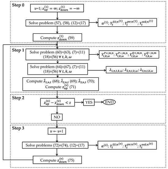
Figure 1. Benders’ decomposition flowchart.

Note that the Benders’ decomposition algorithm described in this section can solve each sub-problem separately, and hence, the computational time of the proposed algorithm grows linearly with the number of scenarios, time blocks, and years, being its scalability excellent.

5. Case Study Data

This section describes the data used for the simulations of the problem explained in Section 3. The Benders’ decomposition method is applied to a 34-bus three-phase radial feeder [21], which has 1 substation, 29 buses with load, and 5 buses with no load. The topology of the system is shown in Figure 2. The data are based on those provided in [18] and [21], but adding new scenarios. In [18] there are 3 levels of demand, wind production, and solar production per each of the 8 time blocks. Now, there are 4 levels and 12 time blocks.

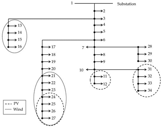
Figure 2. Distribution system under study.

The wind turbines chosen have a capacity of 100 kW and the PV modules have power of 2.5 kW. The candidate buses for each technology are shown in Figure 2 and the maximum power (wind turbine and PV modules) that may be installed at each bus is 250 kW. The maximum number of units is limited to 2 for wind turbines and to 85 for PV modules, and the substation can be expanded adding transformers of sizes ranging from 1 MVA up to a maximum of 5 MVA. Demand increases 2% each year along the planning horizon (20 years). The voltage data of the distribution system is 1 pu in the substation node and the minimum and maximum allowable voltage values are 0.95 pu and 1.05 pu, respectively. The values defined for the interest and discount rates are 8% and 12.5% [6], respectively. Investment data of new devices are shown in Table 2.

Table 2. Investment data.

Unit	Investment Cost [€]	Life Cycle [years]	Tan (φ)
Transformer	20,000	20	0.48
Wind turbines	125,155	20	0.48
PV modules	3445	20	0.48

The operation and maintenance costs of the new renewable production units are €0.007/kWh [8]. The annual budget is €150,000 and the maximum portfolio investment for the life time of the devices is €5,500,000. Data on demand, wind speed, and PV factors used per time block are shown in Table 3, where wind and PV production levels are also displayed. The different levels are combined with each other in every time block. There are four levels of demand, wind, and PV production, hence, the total number combinations (scenarios) per time block is 64. Hence, there are 12 time blocks, 6 per season (winter (October–March) and summer (April–September)), accounting for 768 scenarios. Note that energy prices are not used in scenario generation and each price corresponds with a defined demand factor. These prices are shown in Table 3 and increase 1% each year with respect to the base year. All the levels in each time block have a probability of 1/4. Therefore, the weight of each of the scenarios within each time block is 1/64 [22]. Two blocks are used for piecewise linearization, where the cost of energy not supplied is €15,000/MWh. The tolerance ε of the Benders’ algorithm is specified as €1.

Table 3. Investment data.

Blocks	Hours	Price [€/MWh]	Demand Factors	Wind Speed Factors	Wind Production Factors	Irradiation Factors	PV Production Factors
1	144	70.99	0.92	0.45	1.00	0.78	0.76
		62.89	0.90	0.29	0.76	0.20	0.20
		67.36	0.88	0.17	0.37	0.00	0.00
		57.74	0.87	0.05	0.00	0.00	0.00
2	1108	53.41	0.85	0.49	1.00	0.71	0.70
		48.54	0.82	0.29	0.76	0.17	0.17
		42.94	0.80	0.20	0.45	0.00	0.00
		44.85	0.78	0.08	0.08	0.00	0.00
3	960	45.59	0.77	0.47	1.00	0.76	0.74
		41.21	0.75	0.29	0.77	0.21	0.21
		42.09	0.72	0.19	0.42	0.00	0.00
		42.55	0.69	0.07	0.04	0.00	0.00
4	1029	41.65	0.66	0.48	1.00	0.73	0.71
		39.94	0.62	0.29	0.76	0.22	0.22
		37.11	0.59	0.19	0.44	0.00	0.00
		35.13	0.55	0.08	0.07	0.00	0.00
5	1027	32.37	0.52	0.49	1.00	0.72	0.70
		28.50	0.50	0.28	0.73	0.16	0.16
		23.91	0.49	0.19	0.42	0.00	0.00
		25.36	0.47	0.07	0.04	0.00	0.00
6	112	18.87	0.45	0.43	1.00	0.76	0.74
		16.10	0.44	0.24	0.62	0.18	0.18
		18.35	0.43	0.15	0.30	0.00	0.00
		3.19	0.40	0.05	0.00	0.00	0.00
7	46	57.38	0.97	0.47	1.00	0.76	0.74
		55.58	0.95	0.32	0.85	0.48	0.48
		54.79	0.94	0.19	0.45	0.08	0.08
		53.64	0.93	0.08	0.06	0.00	0.00
8	1083	53.19	0.89	0.44	1.00	0.69	0.67
		52.62	0.85	0.27	0.71	0.27	0.27
		49.51	0.82	0.18	0.41	0.01	0.01
		48.08	0.80	0.07	0.04	0.00	0.00
9	1084	44.25	0.78	0.45	1.00	0.70	0.69
		47.11	0.76	0.28	0.73	0.31	0.31
		44.67	0.73	0.19	0.44	0.02	0.02
		46.98	0.70	0.08	0.07	0.00	0.00
10	1028	47.89	0.67	0.46	1.00	0.71	0.70
		47.16	0.65	0.28	0.74	0.30	0.29
		43.81	0.62	0.19	0.43	0.01	0.01
		42.42	0.58	0.07	0.05	0.00	0.00
11	1025	41.53	0.55	0.47	1.00	0.69	0.67
		39.15	0.53	0.28	0.75	0.26	0.26
		38.14	0.51	0.20	0.46	0.00	0.00
		34.68	0.49	0.08	0.09	0.00	0.00
12	114	34.74	0.47	0.45	1.00	0.64	0.63
		36.49	0.47	0.28	0.73	0.20	0.20
		32.55	0.46	0.19	0.44	0.00	0.00
		33.54	0.44	0.08	0.07	0.00	0.00

6. Results Discussion

Two case studies have been simulated to test the model, where the constraints related to installed power and limits of investment are different. The results of Benders’ algorithm for each case study case are compared with the MILP model given in Equations (1)–(56). These results are obtained using CPLEX 11 under GAMS [23] on an Intel Xeon E7-4820 computer with 4 processors at 2 GHz and 128 GB of RAM. Table 4 presents the numerical results of each simulation in each study case for 768 scenarios. The relative gap is set to 0.01 in all simulations for Benders’ simulation.

Table 4. Total system costs (€).

Case	a		b
	MILP	Benders	MILP	Benders
Total Costs	12,330,870	12,336,090	11,748,580	11,758,350
O&M system costs	11,178,621	11,134,070	9,308,298	9,314,627
Investment costs	1,152,249	1,202,020	2,440,282	2,443,723
CPU time (hours)	742	15	444	24.8

• Case a. Investment limits included: This case represents the most realistic scenario all constraints of the model are taken in account. The first year of the time horizon the renewable technology chosen for investment is photovoltaic (PV), with an installed capacity of 1047.5 kW (see Table 5). The expansion of the substation is carried out in the ninth year, with a new transformer. The new PV devices are installed at the end of the branches because it reduces the costs associated with energies losses. The location of the PV modules within the network is displayed in Table 6. The CPU time decreases by 97.9% when Benders’ decomposition is the method chosen for the simulations.
  Table 5. Power installed (kW) in Case a.

  Case	a
  Year	Substation	Wind	PV
  1	-	-	1047.5
  9	1000	-	-
  Total	2047.5

  Table 6. Nodal allocation of new power installed for Case a.

  Year	Substation		Wind		Photovoltaic
  	Node	No. Units	Node	No. Units	Node	No. Units
  1	-	-	-	-	11 24 25 26 27 31	77 85 85 85 85 2
  9	1	1	-	-	-	-

• Case b. Investment limits not included: in this case, investment constraints (Equations (16) and (17)) are not considered. This new constraint scenario allows the investment in, not only new transformers and PV modules, but also in wind units (see Table 7). Two expansions of the substation are made, in years 9 and 16, PV modules are installed in all candidate nodes, and six wind units, in total, are also installed in the last year. In this case, the new installed capacity is 4725 kW. The location of the PV modules within the network is displayed in Table 8. The CPU time decreases by 94.4% using Benders’ algorithm.
  Table 7. Power installed (kW) in Case b.

  Case	b
  Year	Substation	Wind	PV
  1	-	-	2125
  9	1000	-	-
  16	1000	-	-
  20	-	600	-
  Total	4725

  Table 8. Nodal allocation of new power installed for Case b.

  Year	Substation		Wind		Photovoltaic
  	Node	No. Units	Node	No. Units	Node	No. Units
  1	-	-	-	-	11 12 24 25 26 27 31 32 33 34	85 85 85 85 85 85 85 85 85 85
  9	1	1	-	-	-	-
  16	1	1	-	-	-	-
  20	-	-	21 22 23	2 2 2	-	-

The results are better in Case b than Case a because the problem is less constrained. The introduction of renewable energy in distribution systems reduces the total operation and maintenance (O&M) system costs (see Table 9). The reduction of O&M costs is due a reduction of losses costs and purchase energy by substation. These results highlight the advantages of investing in renewable generation in the long term.

Table 9. Total O&M system costs (€) for 768 scenarios.

Case	a	b	a	b
	MILP	Benders	MILP	Benders
Total O&M Costs	11,178,621	11,134,070	9,308,298	9,314,627
Losses costs	701,609	694,314	598,504	597,734
Not supplied energy cost	13,572	54,010	361	14,866
Purchase energy cost	10,195,660	10,104,480	8,138,853	8,130,402
DG O&M costs	267,780	281,266	570,580	571,625

Finally, Table 10 shows the CPU times required to solve the DGP problem using both the MILP model (1)–(56) and the Benders’ algorithm for different number of scenarios. The CPU time required to solve the MILP model (1)–(56) increases drastically with the number of scenarios (Figure 3 and Figure 4). However, its increment is approximately linear if Benders’ algorithm is considered. This causes that, up to 64 scenarios, MILP model solves the problem faster than Benders’ algorithm but, from 216 scenarios on, Benders’ algorithm becomes a much more efficient way to solve it.

Table 10. CPU Time.

Problem	Case a					Case b
Scenarios	1	8	64	216	768	1	8	64	216	768
MILP	4 s	1.9 m	0.7 h	13 h	742 h	1 s	30 s	3 m	11.1 h	444 h
Benders	36 s	5.3 m	1.7 h	4.9 h	15 h	11 s	90 s	72 m	5.1 h	24.8 h

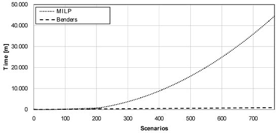
Figure 3. CPU time for Case a.

Figure 4. CPU time for Case b.

7. Conclusions

This paper has considered the DGP problem in a stochastic environment, where both PV and wind technologies as well as demand are subject to random changes. The use of Benders’ decomposition to solve the two-stage stochastic investment problem has allowed us to further decompose the problem by scenarios and planning periods, making it a fully decomposable one. The model has been tested for a 34-bus example with excellent results.

In terms of computing time, the increase in the number of scenarios makes the differences between MILP and Benders’ models evident. Up to 64 scenarios, the MILP model is much faster. Benders’ model needs to perform iterative processes (loops) that increase the computing time. This trend changes as the number of scenarios increases and Benders’ method becomes faster than MILP. In general, MILP’s computing time behaves in a non-linear way, whereas Benders’ model is more linear in terms of computing time. This proves the significant computational advantage of Benders’ with respect to a conventional MILP model.

Note that applying Benders’ decomposition may also allow extending the investment problem to address other relevant issues in distribution systems, such as switching or network reconfiguration. This would be non-viable using the original mixed-integer linear programming problem due to its high computational burden.

The work developed in this article can help investors to decide the kind and size of renewable technologies and the place where install the new devices in the distribution system. As improvements to the proposed problem, other kinds of producers (biomass, hydraulic) can be introduced, incorporate reliability in generation and electric vehicle. In addition, making a comparative with other uncertainty management methods such as K-means.

References

- Payasi, R.P.; Singh, A.K.; Singh, D. Review of distributed generation planning: Objectives, constraints and algorithms. Int. J. Eng. Sci. Technol. 2011, 3, 133–153. [Google Scholar] [CrossRef]
- Viral, R.; Khatod, D.K. Optimal planning of distributed generation systems in distribution system: A review. Renew. Sustain. Energy Rev. 2012, 16, 5146–5165. [Google Scholar] [CrossRef]
- Hadjsaid, N.; Canard, J.F.; Dumas, F. Dispersed generation impact on distribution networks. IEEE Comput. Appl. Power 1999, 12, 23–28. [Google Scholar] [CrossRef]
- Barker, P.P.; De Mello, R.W. Determining the impact of distributed generation on power systems: Part I. Radial distribution systems. IEEE Power Eng. Soc. Summer Meet. 2000, 3, 1645–1656. [Google Scholar]
- Dugan, R.C.; McDermott, T.E.; Ball, G.J. Planning for distributed generation. IEEE Ind. Appl. Mag. 2001, 7, 80–88. [Google Scholar] [CrossRef]
- El-Khattam, W.; Hegazy, Y.G.; Salama, M.M.A. An integrated distributed generation optimization model for distribution system planning. IEEE Trans. Power Syst. 2005, 20, 1158–1165. [Google Scholar] [CrossRef]
- Keane, A.; O’Malley, M. Optimal allocation of embedded generation on distribution networks. IEEE Trans. Power Syst. 2005, 20, 1640–1646. [Google Scholar] [CrossRef]
- Zou, K.; Agalgaonkar, A.P.; Muttaqi, K.M.; Perera, S. Multi-objective optimization for distribution system planning with renewable energy resources. In Proceedings of the ENERGYCON 2010: IEEE International Energy Conference, Manama, Bahrain, 18–21 December 2010; pp. 670–675. [Google Scholar]
- Kagan, N.; Adams, R.N. A Benders’ decomposition approach to the multi-objective distribution planning problem. Int. J. Electr. Power Energy Syst. 1993, 15, 259–271. [Google Scholar] [CrossRef]
- Zakariazadeh, A.; Jadid, S.; Siano, P. Economic-environmental energy and reserve scheduling of smart distribution systems: A multiobjective mathematical programming approach. Energy Convers. Manag. 2014, 78, 151–164. [Google Scholar] [CrossRef]
- Ghasemi, A.; Mortazavi, S.S.; Mashhour, E. Integration of nodal hourly pricing in day-ahead SDC (smart distribution company) optimization framework to effectively activate demand response. Energy 2015, 86, 649–660. [Google Scholar] [CrossRef]
- Hytowitz, R.B.; Hedman, K.W. Managing solar uncertainty in microgrid systems with stochastic unit commitment. Electr. Power Syst. Res. 2015, 119, 111–118. [Google Scholar] [CrossRef]
- Bloom, J.A.; Caramanis, M.; Charny, L. Long-range generation planning using generalized Benders’ decomposition: Implementation and experience. Oper. Res. 1984, 32, 290–313. [Google Scholar] [CrossRef]
- Kim, H.; Sohn, H.S.; Bricker, D.L. Generation expansion planning using Benders’ decomposition and generalized networks. Int. J. Ind. Eng. 2011, 18, 25–39. [Google Scholar]
- Wang, J.; Wang, R.; Zeng, P.; You, S.; Li, Y.; Zhang, Y. Flexible transmission expansion planning for integrating wind power based on wind power distribution characteristics. J. Electr. Eng. Technol. 2015, 10, 709–718. [Google Scholar] [CrossRef]
- Kazempour, S.J.; Conejo, A.J. Strategic generation investment under uncertainty via Benders’ decomposition. IEEE Trans. Power Syst. 2012, 27, 424–432. [Google Scholar] [CrossRef]
- Baringo, L.; Conejo, A.J. Wind power investment: A Benders’ decomposition approach. IEEE Trans. Power Syst. 2012, 27, 433–441. [Google Scholar] [CrossRef]
- Montoya-Bueno, S.; Muñoz, J.I.; Contreras, J. A stochastic investment model for renewable generation in distribution systems. IEEE Trans. Sustain. Energy 2015, 6, 1466–1474. [Google Scholar] [CrossRef]
- Meneses de Quevedo, P.; Contreras, J.; Rider, M.J.; Allahdadian, J. Contingency assessment and network reconfiguration in distribution grids including wind power and energy storage. IEEE Trans. Sustain. Energy 2015, 6, 1524–1533. [Google Scholar] [CrossRef]
- Conejo, A.J.; Castillo, E.; Mínguez, R.; García-Bertrand, R. Decomposition Techniques in Mathematical Programming. Engineering and Science Applications; Springer-Verlag: Heidelberg, Germany, 2006. [Google Scholar]
- Kirmani, S.; Jamil, M.; Rizwan, M. Optimal placement of SPV based DG system for loss reduction in radial distribution network using heuristic search strategies. In Proceedings of the 2011 International Conference on Energy Automation, and Signal (ICEAS), Bhubaneswar, India, 28–30 December 2011; pp. 1–4. [Google Scholar]
- Baringo, L.; Conejo, A.J. Correlated wind-power production and electric load scenarios for investment decisions. Appl. Energy 2013, 101, 475–482. [Google Scholar] [CrossRef]
- Brooke, A.; Kendrick, D.; Meeraus, A.; Raman, R. GAMS/CPLEX: A User’s Guide; GAMS: Washington, DC, USA, 2003. [Google Scholar]
© 2020 by the authors. Licensee MDPI, Basel, Switzerland. This article is an open access article distributed under the terms and conditions of the Creative Commons Attribution (CC BY) license (http://creativecommons.org/licenses/by/4.0/).