Abstract
The recirculation zone and the swirl flame behavior can be influenced by the burner exit shape, and few studies have been made into this structure. Large eddy simulation was carried out on 16 cases to distinguish critical geometry factors. The time series of the heat release rate were decomposed using seasonal-trend decomposition procedure to exclude the effect of short physical time. Dynamic mode decomposition (DMD) was performed to separate flame structures. The frequency characteristics extracted from the DMD modes were compared with those from the flame transfer functions. Results show that the flame cases can be categorized into three types, all of which are controlled by a specific geometric parameter. Except one type of flame, they show nonstationary behavior by the Kwiatkowski–Phillips–Schmidt–Shin test. The frequency bands corresponding to the coherent structures are identified. The flame transfer function indicates that the flame can respond to external excitation in the frequency range 100–300 Hz. The DMD modes capture the detailed flame structures. The higher frequency bands can be interpolated as the streamwise vortices and shedding vortices. The DMD modes, which correspond to the bands of flame transfer functions, can be estimated as streamwise vortices at the edges.
1. Introduction
Lean premixed combustion is one of the major trends for the development of a modern gas turbine combustor to achieve low NOx emissions. In this combustion scheme, the additional air and lower temperature at the flame front may cause instabilities during combustion. To solve this issue, additional recirculation zones must be formed in the combustor to effectively stabilize the flame under different operating conditions. The recirculation zones can provide local flow velocity to balance the turbulent flame speed. In addition, they provide long residence time and a radical pool for continuous burning. Further, the flame can be stabilized in the designed location as a result of the above modifications. Swirling flow is one of the most efficient ways to generate recirculation zones when the value of the swirl number is larger than 0.6 [1].
This recirculation zone normally appears as a result of bubble-type vortex breakdown (VB) [1] or the combined effect of VB and bluff-body stabilization [2]. The bubble type VB can be explained by the hydraulic stability theory [3,4] or critical flow mechanism [5,6]. The most accepted description is that [7], with the quasi-cylindrical approximation, the swirl flow induces the radial pressure gradient, which is balanced with the centrifugal force. The further derivation is related to the adverse axial pressure gradient, which is balanced with the reverse flow. In this theory, the criterion of the swirl number is necessary but not sufficient. The vorticity in the mixing zone changes the velocity direction, which produces the recirculation zone. For instance, when the gas reaches the sudden area jump in the combustor, the negative azimuthal vorticity can be formed due to the diverging of streamlines. Therefore, the turning of the vorticity streams is critical to forming the VB [8]. Geometrically, the burner exit shape and area jump ratio are conducive to the production and stability of bubble type VB. However, the burner exit shape has not been extensively investigated in the modern gas turbine combustor development. Thus, we investigated the influences of the burner exit shape on the flame dynamics by combining statistical methods with computational fluid dynamics.
To simplify the question to only the burner exit shape, three factors are excluded. The first one is the design of the swirl generation. Primarily, the development of the lean swirl combustor was focused on a swirl generator device; for example, the cone shells and slots in the EV (EnVironmental) burners in ABB [9] and Siemens [10] burners, and the axial swirl vane developed from DLE in the LM6000 to DLN series in heavy-duty gas turbines [11]. In this work, the axial swirler with a velocity-based swirl number of 0.4 was applied for all the simulation cases. Secondly, the detailed geometry and pilot nozzles were not included in the center lance design. In the early stage, the center lance was used for water injection to reduce NOx emission. Later, this location was designed with more complicated fuel passages inside for the pilot/diffusion stage to turn down and start the engine flexibly. Finally, the cooling or damping scheme at the front panel location was excluded. Although the local cooling air may change the global stabilization behavior in the combustor and also can change the air distribution and operation concept, it is reasonable to neglect this facility since they are not the focus of this article.
The purpose of this work was to investigate the influence of the burner exit geometry on flame dynamics and distinguish the critical geometry factor. The major influences include the flame structure, heat release rate (HRR), and thermoacoustic characteristic. The geometry of the burner exit is categorized into four geometrical parameters: the expansion ratio (or, combustor diameter), the diameter of the end of the center lance, the diffuser angle, and the shift distance for the center lance. The corresponding flame dynamic characteristic includes parameters such as the heat release rate. As Rayleigh criterion described, when the integral of HRR and pressure fluctuation are larger than the total damping in the system, combustion instability can occur. The pressure fluctuation is mainly influenced by flame structures and chamber acoustics. The latter is influenced by real geometry and boundary impedance, both of which require the detailed design of the combustor. On the other hand, it is more representative to ignore those problems to focus on only the influences of flame structures. The aerodynamically induced flame-stabilization properties and the corresponding frequency response are preserved even when some conditions are simplified. These characteristics reflected by the flame transfer function (FTF) are identified from responsive time series by imposing suitable external excitation at the inlet. The method used to calculate FTF was reported elsewhere [12,13].
However, limited information on how flow structures affect the flame frequency response can be extracted from the FTF. The dynamic mode decomposition (DMD) [14,15,16] method has been applied to explore the potential for the transient flow field data generated by the LES. It is based on the matrix decomposition of the represented coherent structures and can be employed to calculate the frequency band. Notably, the discussion of the DMD results is normally focused on the identification of the low-order structure [17,18,19]. It is unclear whether those structures cause flow or flame instabilities. Therefore, it is necessary to link FTF and DMD results.
In this paper, the influence of the burner exit shape on flame dynamics was investigated. The design of experiments (DoE) method was applied to four critical geometrical parameters. To exactly simulate the flame structures, which are wrinkled by vortices, incompressible large eddy simulation (LES) was performed. Accordingly, time series data and physics fields were acquired from the LES. Then, the question was narrowed down to the spectrum and frequency response of HRR. Nevertheless, the time series were decomposed primarily using seasonal-trend decomposition procedure (STL decompose) to exclude the influence of short physical time. Thus, only data with stationary features in both level and trend were used to calculate the flame response. In particular, the Kwiatkowski–Phillips–Schmidt–Shin (KPSS) tests were performed to identify whether those data were stationary or not. The frequency responses calculated by the flame transfer function were used to match the ones calculated from dynamic mode decomposition (DMD). Finally, the matched frequency bands were found based on their corresponding flame structures. Based on the identification of the flame structures, the geometric tuning was implemented in the design to avoid unexpected frequency bands.
2. Simulation Domain and Setup
2.1. Geometry
In this work, swirl flow was generated using one axial swirler with eight vanes. This swirler was designed for E- or F-class gas turbine combustors and requested to be manufactured by a 3D printing technique named Selective Laser Melting (SLM). Excellent mixing properties of this swirler need also be considered. The swirl vane shape was designed to prevent flow separation. The curved vane had a specific thickness to implement fuel passages inside the vane. The inlet velocity angle was set to 0. The camber turning angle was larger near the tip than that near the root. The designed swirl number was 0.4 based on the velocity swirl number definition. The final shape of the swirl vane is shown in Figure 1. The selected swirl vane height was 15 mm. The axial length of the swirl vane was 30 mm. The center lance radius (R1) was 10 mm, which was selected as the geometrically normalized parameter. One injector was placed on the pressure side and two injectors on the suction side. All the injectors were radially close to the blade tip. The fuel injection occurred perpendicular to the suction surface at the axial location downstream of the thickest airfoil location to maximize the mixing quality between fuel and air. Considering the manufacturing capability of selective laser melting, the directly printed fuel injector should have a diameter greater than 1 mm. Intuitively, better mixing quality can be acquired by employing a longer penetration length of the fuel injection. Thus, the diameter of the nozzle must not be too large. Primarily, nonreactive RANS iterations were used to optimize fuel injection locations based on the mixing quality. Following several RANS iterations, the nozzle diameter was selected as 1.2 mm to fit into the current design. To reduce the computational cost, the fuel injector in the current model was simplified as a cylinder. The fuel inlet boundary was 5 mm upstream of the blade wall surface.
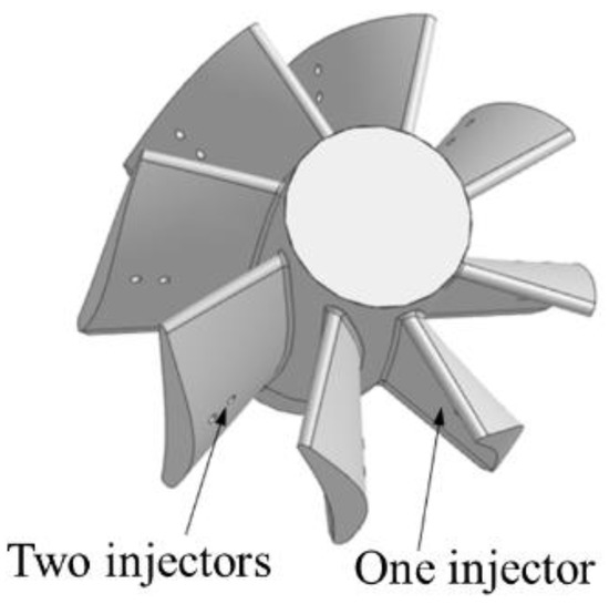
Figure 1.
The 8–vane swirler.
From the domain inlet to the trailing edge of the swirl vane, the geometry was kept the same. As shown in Figure 2, the selected axial length of the mixing zone l = 93.5 mm was from the trailing edge of the swirl vane to the end of the center length. The combustor length L was 380 mm. The radius of the lance tip (R1_TE in Figure 2) was not smaller than the radius of the center lance because the lance tip can potentially be used as a pilot stage or for oil injection or bluff-body stabilization.
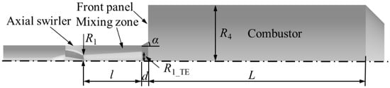
Figure 2.
Geometric control parameters for the DoE study.
2.2. DoE Case Series
As shown in Figure 2, to explore the influence of geometric parameters on the flame behaviors, four parameters were selected as critical design parameters.
- The distance (d) from the center lance tip to the front panel. This parameter is a critical parameter in dual fuel engines when the liquid fuel is injected from the center lance tip. d/2R1 is selected as the notation.
- The diffuser angle (α), which controls how the burner discharges flow into the combustor. Apparently, under the current swirl number, the larger the angle, the wider the center recirculation zone (CRZ). However, this change might also lead to a smaller outer recirculation zone (ORZ) and weaker neighboring flame interaction in the multi-burner arrangement. A larger or diffuser angle may lead to flow separation in the burner. Nevertheless, it is difficult to predict the precise value if the swirl flow is presented. Thus, the upper limit value (30°) was applied in the current paper.
- The expansion ratio, which is calculated as the cross-sectional area ratio of the combustor to the burner. The formation of the CRZ shape can be influenced by this parameter. To simplify the notation, we used R4/R1.
- The diameter of the center body back surface (R1_TE), which is related to the bluff-body-induced recirculation zone, is also selected as the design parameter. R1_TE/R1 is selected as its notation.
With a two-level full factorial DoE, a total of 16 geometric variants need to be investigated (Table 1).

Table 1.
Two–level full factorial design table.
2.3. CFD Setup
2.3.1. Boundary and Mesh
The simulation domain was the 45° sector with a periodic boundary. Although the current simulation setup can prevent high simulation costs, the azimuthal phenomena, for example, the processing vortex core cannot be predicted. The boundary conditions were determined, considering the premixed burner design in F-class gas turbine. The exact value was tested using reactive RANS. Reynolds number at the burner inlet was over 22,000, and the equivalence ratio was 0.514 based on the current inlet boundary condition shown in Table 2.
Table 2.
Inlet boundary conditions for the CFD analysis under ambient conditions
A hybrid mesh was employed for calculation. All wall boundaries were resolved by three-layer prism meshes. Different regions were resolved by various mesh sizes. The mixed zone, swirler and upstream of the combustor were refined to distinguish the mixing and flame details and the corresponding mesh resolutions were 0.35, 0.2 and 0.35 mm, respectively. The resolution of the combustor downstream was enlarged to 1.0 mm due to focusing on the burner exit. Around 7.7 million cells were generated for case 12 and Figure 3 shows the total mesh and local details for this case. With respect to the mesh dependence, a posteriori method based on the energy index theory [20] was applied to determine whether the mesh was fine enough for LES calculation. Firstly, the integral length scale () extracted from the RANS simulation is regard as a prior-grid estimator. Less than 1/10 of this length scale is selected as the first trail mesh resolution. The Celik-defined energy-based index M [21,22] is defined as follows:
where k is the turbulent kinetic energy, subscript res and sgs denote resolved and subgrid-scale model. The energy dissipation from the numerical discretization was neglected resulting from the application of the bound center scheme. The simulation was considered valid when the energy index M was over 85% [20]. The contour of the index M in the center plane is presented in Figure 4. The index value was almost larger than 85% in the entire flow domain except the outlet region. Since this work was focused on the burner exit shape, the mesh was considered adequate for this purpose.
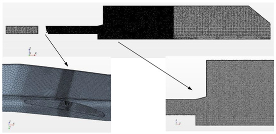
Figure 3.
Mesh scheme and local details (Case 12).
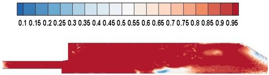
Figure 4.
Contour of the index M for case 12 in the center plane.
2.3.2. Numerical Procedures
The Favre-filtered equations for mass and momentum are introduced as follows:
where is the filtered pressure, is the filtered mixture density. represents the subgrid-scale stress tensor, which is calculated by the Smagorinsky model as follows:
where denotes the kinematic viscosity and is the rate-of-strain tensor in the filtered format. is the model constant and is the filter width.
In LES, the wall-adapting local eddy-viscosity model [23] was used as a subgrid-scale model. At the air and fuel inlets, the “no perturbations” were set for turbulence flow because the air inlet was implemented with inlet mass flow excitation. Synthesizer methods would dilute the excitation signal with a high frequency range. Another reason is that the flame dynamics induced by coherent structures are discussed in the following sections. Thus, very low turbulence was applied at both inlets to prevent high frequency turbulent flow. The bounded center difference scheme was applied for momentum, progress variable (PV), and mean mixture fraction discretization. The second-order simplicity scheme was applied in transient formulation. Turbulent flame closure (TFC) under partially premixed conditions was selected as the combustion model in ANSYS FLUENT. In TFC model, the flame front was as PV = 1. The Favre average transport equation for PV was resolved in LES. Its source term was modelled with the turbulent flame speed (). In the TFC model, was calculated by Damköhler number () and turbulent velocity. The GRI 3.0 [24] mechanism was used for tabulation. Heat loss was not considered in the current paper.
Two LES calculations were conducted for each case. The first LES calculation was performed based on the converged reactive RANS equations. After 0.1 s of the first LES, the second LES was performed with an inlet velocity excitation with a duration of 0.25 s. These two durations were selected based on the convection time from the inlet burner flame location to combustor outlet (flow-through time) and the amplitude shape of the excitation signal in the frequency range lower than 800 Hz. The precision of LES was validated in an indirect way shown in Appendix A, where large eddy simulations of a V-type bluff body stabilized premixed combustion employing the same flow and combustion models with those in this paper were compared with experimental results in previous literature.
3. Postprocessing Algorithms
3.1. Flame Transfer Function
The FTF calculation was based on the assumption that a partially premixed flame is a time-invariant (LTI) linear system excited by low amplitude signals from which the frequency response of the system can be extracted. The excitation was implemented with air mass flow rate at the burner inlet. Originally, this fluctuation was caused by the turbulent HRR inside the combustor and when it propagated upward into the air plenum, it caused air mass flow rate fluctuations. In the frequency domain, the signal showed no drop in amplitude in the range up to 800 Hz. This signal was multiplied by the 105% inlet mass flow rate to produce the value applied at the inlet boundary.
The inlet excitation signal used a discrete random binary signal (DRBS) [25,26,27], which had been used in a laboratory-scale combustor [28,29] and industrial gas turbines [30]. The properties of this signal in the time and frequency domain are shown in Figure 5. The selected shape of the signal has a clear amplitude to limit the flame blow-off issue and flashback risk. The signal intensity should be neither too large, which would lead to flame blow-off, nor too small, so that it cannot transport to the flame front. The excitation had a 5% amplitude, which was suitable for this combustor, and its duration was 0.25 s.
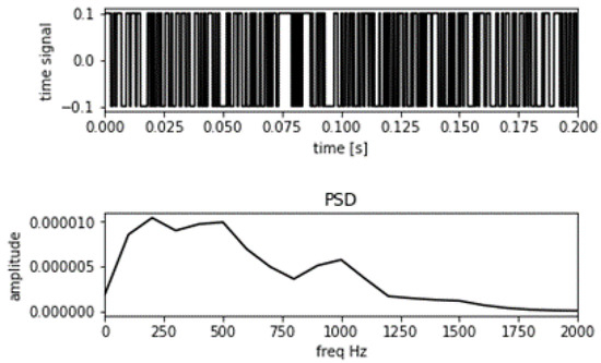
Figure 5.
Discrete random binary excitation signal.
The FTF is calculated as follows [31]:
where (ˆ) represents the fluctuation value, (ˉ) represents the average value, ω is the angular frequency, is the heat release rate fluctuation calculated as the volume integral of the product formation rate over the simulation domain and is the velocity perturbation at the inlet. This equation is performed by solving the relation between the cross-correlation of the numerator and denominator and the autocorrelation of the denominator.
3.2. Dynamic Mode Decomposition
Without explicitly comprehending the governing equation, DMD is an effective method that can reveal dynamic process through the operator matrix [13,14,15]. The algorithm of DMD contains two aspects: one is using the singular value decomposition (SVD) to reduce the computational cost of matrix decomposition. The other is using the Fourier mode concept to separate dynamic modes from the background mean field. The flame information reflected by the product formation rate is extracted as a vector from LES with constant interval. Concatenate vectors along time to form the data matrix, which can be separated into (−1) and (). where is the time. If the time step is small enough (0.2 ms in this case), one step forward dynamics can be estimated as a linear operator M and Y = MX. Then, is multiplied with both sides of the equation to deduce , which leads . The dynamics information can be obtained by analyzing the operator A. Then, implement SVD of that
Here, is the left-singular vector of , is the right-singular vector of is the singular value formed diagonal matrix, represents the spatial resolution of the flame, and is the collected snapshots. Superscript * is the conjugate transpose operator. When applying the snapshot method, the value of should be large enough to cover flame evolution time, but should also be small enough that the postprocessing machine can afford it. Current value is 1001. Calculating the SVD of has a high computational cost. The solution for this is to project on matrix , which leads to a low-rank . has the same singular value as . Then, . Eigen decompose matrix as in which is the singular vector, is the singular value diagonal matrix, and is the rank. The dynamic mode is calculated as . The temporal growth rate for DMD mode is calculated as in which is the real part. The frequency of DMD is calculated as a Fourier mode as in which is the imaginary part.
3.3. Statistical Method for Time Series Analysis
It might be difficult to estimate the combustion in the final status for two reasons. Firstly, the time step in LES is small since the cell size is small. It prevents the LES simulation time lasting long enough or providing sufficient evidence to view the quenching of the flame. Secondly, the time series fluctuate due to the coherent structures and background turbulence. To provide statistically meaningful analysis and prevent empirical results, the seasonal-trend decomposition procedure based on Loess (STL) algorithm [30] is proposed. Suppose the time series of the volume integral of PFR () can be decomposed into level (), trend (), nonstationary part (), and stationary part ().
As shown in the above equation, the linear trend () is assumed in the current cases. If , then the time series is stationary if , and level is stationary if . Then, the Kwiatkowski–Phillips–Schmidt–Shin (KPSS) test [32,33], is introduced here to check the unit root. This test is used to validate if there is a unit root, which means the series is nonstationary. The nonstationary characteristics leads to spurious regression in the statistical models. Compared to the conventional unit root test such as the Dickey–Fuller test (DF test), the KPSS test can reject null hypothesis, indicating that there is not sufficient evidence to say there is no unit root. So, the statistical hypothesis in the KPSS test is as follows:
First situation, where the null hypothesis is Then, the time series is level stationary. The second situation, where the null hypothesis is Then, the time series is trend stationary. The alternative hypothesis is . Under the null hypothesis, parameter can be estimated using ordinary least squares regression and is the residual. Then, the series (). Accordingly, the KPSS statistic can be calculated as follows:
Here, , in which . Parameter represents the time lag.
4. LES Results
4.1. Ensembled Average Results on Flame and Flow Field
The ensembled average of the axial velocity in snapshots and the RMS results are plotted in Figure 6 and Figure 7, respectively. Figure 8 and Figure 9 illustrate the corresponding PV results. The parameter, PV, was selected to represent the process of reaction. The region where 0 < PV < 1 is due to the averaged process with instantaneously shedding unburnt mixture into burnt gases. In general, contours of axial velocity (Figure 6) show that ORZ and CRZ exist in all cases. Contours of PV (Figure 8) show that the flames can be separated into outer and inner branches. All the flames anchor at the edge of the centerbody. The outer branch follows the diffuser angle of the inner mixing zone and burns in the combustor. The anchoring point is the edge connecting front panel and combustor.
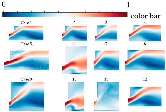
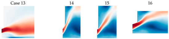
Figure 6.
Ensembled average axial velocity.
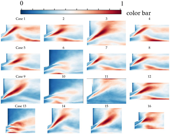
Figure 7.
RMS axial velocity.
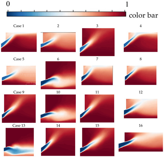
Figure 8.
Ensembled average PV field
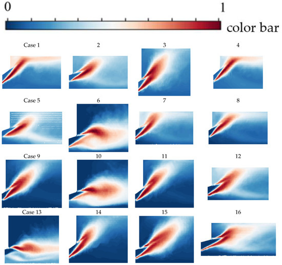
Figure 9.
RMS PV field.
In cases 6, 10, and 13, the fluid with high axial velocity was pressed inwards to the centerline. The corresponding contour plots of axial velocity RMS (Figure 7) show high level fluctuation in the axisymmetric line, which indicates the change in the length of the CRZ. There was a specific level of axial velocity RMS at both inner and outer branches of the flame. The contours of mean PV in these cases showed a high level of PV in the ORZ but a low level of PV in the CRZ region. This was confirmed in the contours of RMS PV plots where the high fluctuation of PV was located at the outer branch of the flame, indicating a strong mixing between ORZ and the flame.
Except these three cases, all cases showed the axial velocity flow outwards to the combustor wall. In cases 1, 2, 4, 5, 7, 8, and 12, the stream impinged to the wall and then turned its direction toward the stream. The corresponding axial velocity RMS results showed a high level of fluctuation at the inner branch of flame and axisymmetric line. This indicated the mixing behavior between the inner branch of the flame and CRZ. This conclusion was confirmed from the contours of mean PV results. In these cases, the PV = 1 in the CRZ region, but the PV values were less than 1 in the ORZ region.
In cases 3, 9, 11, 14, and 15, there was no strong impinging toward the combustor wall indicated from the contours of the mean axial velocity. The contours of RMS PV indicated a strong mixing between both flame branches and recirculation zones. The 16 cases could be divided into three groups as shown in Table 3. Comparing the flame types with the geometric parameters by using ANOVA model, we found that there was no strong impact parameter for the formation of type-A flame and R4/R1 was the only important factor that influenced the formation of type-B flame. The smaller level of R4/R1 would lead to the type-B flame. R4/R1 also influenced of the formation of type-C flame. The larger level of R4/R1 would lead to the type-C flame.
Table 3.
Flame categories of the 16 cases using LES results.
4.2. Time Series Results
The LES cases were obtained from reactive steady RANS results. In RANS, the averaged static temperature at outlet was 1727 K with 4.22 K standard deviation. However, when the LES was enabled and fully developed, the arithmetic averaged static outlet temperature in 16 cases dropped due to the shedding of the unburnt mixture. With sampling time of 0.2 s, the averaged value from 16 cases was 1640 K, which was 5% lower than the RANS result. The averaged static temperature at outlet in each case was compared with the mean value of 1640 K in Figure 10. The volume integral of product formation rate (PFR) in each case was compared with arithmetic mean one in all 16 cases.
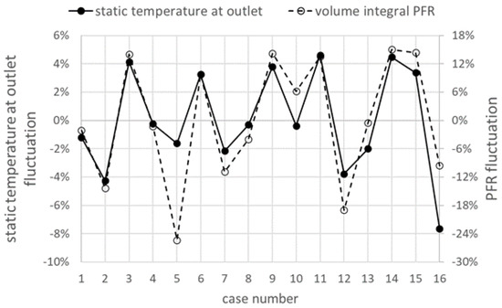
Figure 10.
Fluctuations of the static temperature at outlet and the volume integral PFR.
The comparison between the outlet static temperature in each case and the averaged value are shown in Figure 10. It shows similar trend and level as the PFR. The fluctuation level of volume integral of PFR was three times larger than that of outlet temperature, except for cases 5, 12, and 16. In case 5, the fluctuation level in PFR was 12 times larger than that in the temperature. Comparing the three types of flame in Table 3, the type-C flame cases (3, 9, 11, 14, and 15) all showed higher temperature at the outlet and integral PFR compared with the arithmetic averaged values among the 16 cases. The type-B flame cases (1, 2, 4, 5, 7, 8, 12, and 16) all showed similar or lower values of temperature and PFR compared to the averaged levels. The values in type-A flames (6, 10, and 13) showed uncertainty in relation to case-averaged values. The above results indicate that there is shedding unburnt mixture into combustion chamber in the cases of type-B and A as presented in Figure 11.
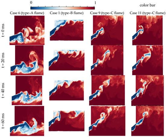
Figure 11.
Instantaneous contours of PV sampled every 20 ms in four cases.
The p-values tested for level and trend in 16 cases are summarized in Table 4. As shown in Table 4, the levels of the p-value were smaller than 0.01 in all the cases, except cases 3, 6, and 14. The p-value of case 6 was also close to 0.01. This meant that we could reject the null hypothesis in cases 3 and 14. Furthermore, it meant all the cases except these three were not level stationary. The trend p-values were smaller than 0.01 in all cases, except cases 9 and 11. This meant that, except cases 9 and 11, the rest of the cases were not stationary. The p-values in all cases were larger than 0.1 after the first-order difference. This meant that it could not reject the differenced time series of those cases that were level or trend stationary. It indicated that the heat release levels in cases 3, 6, and 14 were stationary. The heat release level changed in cases 9 and 11, but the trend of heat release rate stayed the same.
Table 4.
p–value for level and trend in 16 cases.
Furthermore, to investigate the trend from the fluctuations, the turbulence and coherent structure were separated using the spectrum. Considering the size of the flow structures, we deduced that the large-scale coherent structures had lower frequency bands than those in the turbulence, which had high frequency bands and behaved like noise.
As shown in Figure 12, the selected time series of heat release was decomposed into level, trend, seasonality, and residual. The frequency for decomposition was set to 2000 Hz. It meant that the frequency band lower than 2000 Hz was captured in seasonal data. As shown in case 1, the heat release rate showed a general trend of reducing level after 0.07 s. The spectrum indicated fluctuations near 570 Hz and 1340 Hz. In case 6, the spectrum showed the heat release rates fluctuating around 1000 Hz and 1340 Hz. In case 11, the spectrum showed 1340 Hz. In case 15, the heat release rate level was increasing in the trend. This was the reason that even the outlet temperature and heat release rate was higher than the overall level among 16 cases shown in Figure 12, the p-value in the KPSS test concluded it was a nonstationary time series, which was different from the other cases in type-C flame.
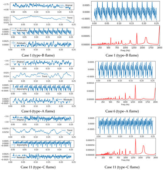
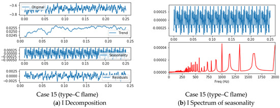
Figure 12.
Level, trend, seasonality, residual and spectrum of the seasonality of decomposed time series for three types of flames.
4.3. Frequency Domain Results
As illustrated in the previous section, only cases 3, 9, 11, and 14 had the potential to do FTF. As shown in the FTF in Figure 13, the gain and amplitude were plotted in the frequency band less than 500 Hz since the excitation signal was limited to less than 800 Hz. The FTF higher than 800 Hz was not plotted. Meanwhile, the gain was less than 1 in the frequency range higher than 300 Hz. Thus, the flame behaved as a low-pass filter that flames responsed to excitations of only less than 300 Hz.
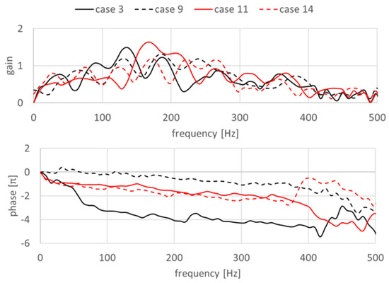
Figure 13.
The gain and phase of FTF for cases 3, 9, 11 and 14: gain (top) and phase (bottom).
As shown in the FTF plots, in all the four cases, the gain values were almost zero when the frequency reached zero. The shape of the gain curves was wavy. The higher gain range was 88–192 Hz in case 3, and 152–224 Hz in Case 11. The higher gain values were in the range 100–300 Hz in cases 9 and 14. Based on the n - τ model, when the residence time was approximately 2 ms in the current case, the gain plot showed a wave shape. The first peak was near 250 Hz, and the first trough near 450 Hz. Nevertheless, there were multiple peaks in the range of less than 450 Hz. This could be explained by the flame responses from two resources. One was due to the large motion flame being rolled-up, which was caused by inlet axial excitation and vortex shedding. The other source was the flame angle changed due to the swirl number changes [34]. This swirl number change was induced by the fluctuation both in tangential velocity and axial velocity, in which, the tangential velocity was induced when the axial perturbations passed through the swirl vane [35]. Assuming a linear combination of the two responses, which has been extensively discussed in previous work [36], if the phase between the two responses is close, the HRR is higher. If the two responses are out of phase, the integral one is lower [37]. However, there is no propagation time for the acoustic wave under the incompressible condition. Thus, the axial velocity perturbation and the azimuthal perturbation induced by the swirler reach the flame front at nearly the same phase. There were only the coherent structure influences in the current work because the incompressible condition was set in CFD.
Comparing cases 9 with 11, which show a similar response function in the frequency range 50–150 Hz, it indicates that the diameter of the centerbody trailing edge (R1_TE/R1) and the shift distance (d in Table 1) might not strongly influence parameters for FTF in this band. Comparing cases 3 with 11 showed a distinguishable response function in 50–250 Hz, indicating that the combustor size (R4/R1) was a non-negligible factor. Further conclusions require more statistical samples.
Comparing the phase curves in the four cases shown in Figure 13, in the very low-frequency range (<15 Hz), cases 3, 11, and 14 showed the inertia behavior in the transfer function; meanwhile, this inertia element was not shown in case 9. Near 50 Hz, only case 3 indicated the oscillation element. Near 400 Hz, case 14 indicated a second differential element. Since the gain value was small when the frequency was higher than 400 Hz, the phase was not accurate enough to analyze. Except for the above four cases, transfer functions of other cases were not studied because the flame might finally quench after a long time. With level or trend changing over time, there will be inconsistencies in the low-frequency range.
4.4. Dynamic Mode Decomposition Results
By using time series decomposition, the interesting frequency bands were limited to three, which indicated the fluctuation of the heat release rate. By using the flame transfer function, the frequency bands, which potentially make the flames behave like amplifiers, were selected. To understand the regular flame structures in three flame types, cases 1, 6, and 11 were selected, and the snapshots in those cases were postprocessed using the DMD method. DMD results can give a single frequency for each mode and the corresponding growth rate. Table 5 presents the first 50 modes’ results, which are ordered based on the growth rate decay. Since the DMD modes are in pairs with opposite frequency signs, the below table shows only the positive frequency modes with a frequency band in the range 0–2000 Hz.
Table 5.
Frequency and growth rate (G.R.) for each DMD mode in three cases.
As shown in Table 5, each case had at least one zero-frequency mode. The frequency is calculated as , if there is no imaginary part in the eigenvalue, the frequency is zero. The flame is more like a drift motion reflected by the DMD modes. The detailed analysis of DMD modes was selected according to three principles: (1) the highest growth rate, which was a zero-frequency mode in all three cases; (2) the DMD modes which had frequency bands corresponding to the spectrum of the seasonal part of PFR; (3) the DMD modes which had frequency bands corresponding to the spectrum showing a high gain in the FTF. Figure 14 lists the selected four modes in cases 1, 6, and 11.
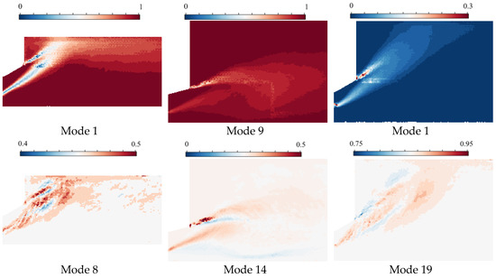
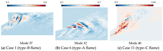
Figure 14.
Four DMD modes of cases 1, 6, and 11.
As shown in Figure 14, the high growth rate modes in each case had a similar mode shape. Case 1 was selected to represent the type-B flame. The highest PFR concentrated at two edges, the edge of the centerbody, and the edge connect burner and front panel. They represented the main part of averaged PFR fields. The two branches of the flame impinging to the combustor wall. The 8th and 37th DMD modes fluctuated with 565 Hz and 1336 Hz, which were close to the 570 Hz and 1370 Hz peaks in the seasonal part of the PFR spectrum, respectively. The 8th mode shape represented the two streams of the vortices shedding at the two edges, and these two streams merged in the combustor. Case 6 was selected to represent the type-A flame. As shown in the 9th mode, the highest PFR was located at the edge that connected the burner and front panel. The inner flame branch had a lower PFR. The 14th mode was constant as well. There was a lower concentrate of PFR near the root of the outer flame branch. The fluctuating mode was the 12th mode, which was 997 Hz. This mode represented that the shedding motion of the outer branch was stronger than the inner branch. This shedding motion could explain the 1000 Hz peak fluctuating in the seasonal series of PFR. Compared with case 1, the fluctuating motion in the inner flame branch was much weaker and merged into CRZ. Case 11 was selected to represent the type-C flame. The 1st mode was the stationary mode, which represented the high concentrate of PFR at two edges. There were no DMD modes that had similar frequency bands like those in the spectrum of the seasonal time series because the selected DMD modes in Table 5 were sorted by the growth rate. The lower the growth rate, the more stable the mode was. Instead, the 19th and 40th modes were selected since they corresponded to the frequency bands in the higher gain of FTF. The 19th mode indicated the PFR rotating streamwise at two edges. The 40th mode was difficult to interpolate. In the engine development work, the frequency close to 191 Hz could be captured by the confined domain and create vibration. Then, the PFR located at two edges might be modified, for example, by adding cooling air injection locally.
In short, the DMD processing method provides three useful pieces of information. Firstly, the frequency is calculated from the eigenvalue. It indicates whether the mode is fluctuating or not. Meanwhile, the value can be linked to the spectrum calculated from the time series, for example, from the FTF, the spectrum of HRR directly. Secondly, the growth rate result, which is also calculated from the eigenvalue. It indicates whether the mode is stable or not. Finally, the DMD mode shape. It indicates the location and fluctuating motion of the mode, which helps the mechanical design of the combustor.
5. Conclusions
This paper presents the LES results for a series design of a burner exit. The geometric design space of the burner exit shape is limited to four design parameters: the radius of the lance tip (R1_TE), the radius of the combustor (R4), the diffuser angle (α), and the lance recess distance (d). A two-level full factorial design with 16 variants was generated and simulated using the LES methods. Firstly, the classification was made according to the average and RMS of the LES field. Three types of flames were defined. The corresponding control parameters to form those three types were determined by the statistical method. We found that the R4/R1 is the most important parameter that determines the formation of type-B or type-C flames. The larger value of the R4/R1 would lead to the formation of a type-C flame, whereas the smaller value leads to the formation of a type-B flame. The averaged outlet temperature and volume integral of PFR were compared among the 16 cases.
The results indicated that even the outlet temperature in all 16 cases showed less than 5 K standard deviation in RANS results, the averaged values in LES were lower than those in the RANS and had a much larger deviation. One possible reason is that the unburnt mixture shedding into the combustor leads to locally low PFR. Irrespective of whether this unburnt mixture would finally burn in the downstream or not, the averaged PFR will be lower. The low outlet temperature would also link to this reason. In current cases, if there is a continuously unburnt mixture mix with burnt gases, there is potentially the flame that can quench it. However, it is not obvious from the LES result, which is limited by a short computational time and high turbulence in the signal. Thus, the KPSS test was introduced to estimate if the PFR series was stationary or not. Results indicated that, except for the type-C flames, all other flames were nonstationary, either in level or trend. By decomposing time series into level, trend, seasonality, and residual, the spectrum could be obtained using seasonal time series. These spectra showed 570 Hz, 1000 Hz, and 1340 Hz peaks due to the fluctuating structural flame shapes. The forced flame response was represented by flame transfer functions. The FTF results showed that in the range 100–300 Hz, the swirl flame responded to external excitation. Thus, in this range, the flame may behave as an amplifier in the combustion system. To understand the flame structures, which corresponded to those frequency bands, the dynamic mode decomposition was performed. The DMD modes captured the detailed flame structure corresponding to each frequency. Based on DMD modes, the higher frequency bands could be interpolated as the streamwise vortices and shedding vortices at the geometry edges. The DMD modes, which corresponded to FTF bands, could be estimated as streamwise vortices at the edges.
The characteristics of combustion instabilities for a certain combustor can be approached by the above techniques. When combustion instability emerges, the structure of this combustor can be rationally tuned according to the relationship between geometric parameters and instability risks at the design stage. Meanwhile, combustors which have high risks for instabilities can be avoided. Corresponding experimental validations will be carried out in the future. This work is mainly focused on gas turbine combustors which have lower frequencies and mean flow velocity than those in rocket combustors. The proposed analysis techniques will be extended to consider combustion instabilities in rocket combustors in future work.
Author Contributions
Both authors contributed to the study conception and design. Material preparation, data analysis and manuscript were performed by Y.Y. Then the manuscript was revised and complemented by Z.Y. Both authors have read and agreed to the published version of the manuscript.
Funding
This research was funded by Chinese Academy of Sciences (CAS) Pioneer Hundred Talent Program, grant number Type-B Y9291282U1.
Conflicts of Interest
The authors declare no conflict of interest.
Appendix A
Large eddy simulations of a V-type bluff body stabilized premixed combustion employing the same flow and combustion models with those in this paper were compared with experimental and RANS results in reference [38] to validate the precision of LES. The simulation domain in this reference is presented in Figure A1, which consists of an equilateral triangle bluff body. Axial average velocity and temperature profiles from experimental data, RSM model, k-ε model and LES results are depicted in Figure A2 and Figure A3, respectively. LES results were performed in this work, while other data were directly extracted from the reference. Results indicated that the central axial velocities were overestimated or underestimated by the k-ε or RSM model. Axial velocity profiles calculated by LES could match the experimental data better than those by RSM or k-ε model. Center velocity distributions were more accurate in LES results. With respect to mean temperature profiles, the discrepancy of central temperature was minor between LES results and experimental ones.

Figure A1.
Simulation domain of the bluff body stabilized premixed combustion in reference [38] (dimensions in mm).
Figure A1.
Simulation domain of the bluff body stabilized premixed combustion in reference [38] (dimensions in mm).


Figure A2.
Comparison of axial average velocity profiles for experimental data, RSM model, k-ε model results in reference [38] and LES results in this work (top: x = 0.15 m section; bottom: x = 0.376 m section).
Figure A2.
Comparison of axial average velocity profiles for experimental data, RSM model, k-ε model results in reference [38] and LES results in this work (top: x = 0.15 m section; bottom: x = 0.376 m section).


Figure A3.
Comparison of average temperature profiles for experimental data, RSM model, k-ε model results in reference [38] and LES results in this work (top: x = 0.15 m section; bottom: x = 0.35 m section).
Figure A3.
Comparison of average temperature profiles for experimental data, RSM model, k-ε model results in reference [38] and LES results in this work (top: x = 0.15 m section; bottom: x = 0.35 m section).

References
- Gupta, A.K.; Lilley, D.G.; Syred, N. Swirl Flows; Abacus Press: Tunbridge Wells, UK, 1984. [Google Scholar]
- Stein, O.T.; Kempf, A.M. LES of the Sydney swirl flame series: A study of vortex breakdown in isothermal and reacting flows. Proc. Combust. Inst. 2007, 31, 1755–1763. [Google Scholar] [CrossRef]
- Leibovich, S. Vortex stability and breakdown-survey and extension. AIAA J. 1984, 22, 1192–1206. [Google Scholar] [CrossRef]
- Leibovich, S. Vortex Breakdown: A Coherent Transition Trigger in Concentrated Vortices; Springer Science & Business Media: Berlin, Germany, 1991. [Google Scholar]
- Squire, H.B. Analysis of the Vortex Breakdown Phenomenon, Part I. Aero; Report; Imperial College: London, UK, 1960. [Google Scholar]
- Benjamin, T.B. Theory of the vortex breakdown phenomenon. J. Fluid Mech. 1962, 14, 593–629. [Google Scholar] [CrossRef]
- Delery, J.M. Aspects of vortex breakdown. Prog. Aerosp. Sci. 1994, 30, 1–59. [Google Scholar] [CrossRef]
- Brown, G.L.; Lopez, J.M. Axisymmetric vortex breakdown Part 2. Physical mechanisms. J. Fluid Mech. 1990, 221, 553–576. [Google Scholar] [CrossRef]
- Döbbeling, K.D.; Hellat, J.; Koch, H.C. 25 Years of BBC/ABB/Alstom Lean Premix Combustion Technologies. In Proceedings of the Turbo Expo: Power for Land, Sea, and Air, Charlotte, NV, USA, 6–9 June 2005. [Google Scholar]
- Hermsmeyer, H.; Prade, B.; Gruschka, U.; Schmitz, U.; Hoffmann, S.; Krebs, W. V64. 3A gas turbine natural gas burner development. In Proceedings of the Turbo Expo: Power for Land, Sea and Air, Amsterdam, The Netherlands, 3–6 June 2002. [Google Scholar]
- Schlein, B.C.; Anderson, D.A.; Beukenberg, M.; Mohr, K.D.; Leiner, H.L.; Traptau, W. Development history and field experiences of the first FT8 gas turbine with dry low NOx combustion system. In Proceedings of the International Gas Turbine and Aeroengine Congress and Exhibition, Indianapolis, IN, USA, 7–10 June 1999. [Google Scholar]
- Gentemann, A.; Hirsch, C.; Kunze, K.; Kiesewetter, F.; Sattelmayer, T.; Polifke, W. Validation of flame transfer function reconstruction for perfectly premixed swirl flames. In Proceedings of the Turbo Expo: Power for Land, Sea and Air, Vienna, Austria, 14–17 June 2004. [Google Scholar]
- Yang, Y.; Liu, X.; Zhang, Z.H. Large eddy simulation calculated flame dynamics of one F-class gas turbine combustor. Fuel 2020, 261, 116451. [Google Scholar] [CrossRef]
- Yang, Y.; Liu, X.; Zhang, Z.H. Analysis of v-gutter reacting flow dynamics using proper orthogonal and dynamic mode decompositions. Energies 2020, 13, 4886. [Google Scholar] [CrossRef]
- Schmid, P.J.; Sesterhenn, J. Dynamic mode decomposition of numerical and experimental data. J. Fluid Mech. 2008, 656, 5–28. [Google Scholar] [CrossRef]
- Rowley, C.W.; Mezic, I.G.O.R.; Bagheri, S.; Schlatter, P.; Henningson, D. Spectral analysis of nonlinear flows. J. Fluid Mech. 2009, 641, 115–127. [Google Scholar] [CrossRef]
- Huang, C.; Anderson, W.E.; Harvazinski, M.E.; Sankaran, V. Analysis of self-excited combustion instabilities using decomposition techniques. AIAA J. 2016, 54, 2791–2807. [Google Scholar] [CrossRef]
- Paul, P.; Milos, I.; Robert, C. Transient and limit cycle combustion dynamics analysis of turbulent premixed swirling flames. J. Fluid Mech. 2017, 830, 681–707. [Google Scholar]
- Wilhite, J.M.; Dolan, B.J.; Kabiraj, L.; Gomez, R.V.; Gutmark, E.J.; Paschereit, C.O. Analysis of combustion oscillations in a staged MLDI burner using decomposition methods and recurrence analysis. In Proceedings of the 54th AIAA Aerospace Sciences Meeting, San Diego, CA, USA, 4–8 January 2016. [Google Scholar]
- Celik, I.B.; Cehreli, Z.N.; Yavuz, I. Index of resolution quality for large eddy simulations. J. Fluids Eng. 2005, 127, 949–958. [Google Scholar] [CrossRef]
- Celik, I.; Klein, M.; Janicka, J. Assessment measures for engineering LES applications. J. Fluids Eng. Trans. 2009, 131, 031102. [Google Scholar] [CrossRef]
- Geurts, B.J.; Fröhlich, J. A framework for predicting accuracy limitations in large-eddy simulation. Phys. Fluids 2002, 14, L41–L44. [Google Scholar] [CrossRef]
- Ansys. Fluent 17.0 Theory Guide; Ansys Inc.: Canonsburg, PA, USA, 2015. [Google Scholar]
- Berkeley Mechnical Engineering. Available online: http://www.me.berkeley.edu/gri_mech/ (accessed on 12 June 2019).
- Polifke, W.; Paschereit, C. Determination of thermos-acoustic transfer matrices by experiment and computational fluid dynamics. ERCOFTAC Bull. 1998, 38, 1–3. [Google Scholar]
- Huber, A.; Polifke, W. Dynamics of practical premixed flames, part II: Identification and interpretation of CFD data. Int. J. Spray Combust. Dyn. 2009, 1, 229–249. [Google Scholar] [CrossRef]
- Polifke, W.; Poncet, A.; Paschereit, C.O.; Döbbeling, K. Reconstruction of acoustic transfer matrices by instationary computational fluid dynamics. Sound Vib. 2001, 245, 483–510. [Google Scholar] [CrossRef]
- Hilares, T.W.C.; Roberto, L. Numerical Simulation of the Dynamics of Turbulent Swirling Flames. Ph.D. Thesis, Technische Universität München, Munich, Germany, 2012. [Google Scholar]
- Bothien, M.; Lauper, D.; Yang, Y.; Scarpato, A. Reconstruction and analysis of the acoustic transfer matrix of a reheat flame from large-Eddy simulations. In Proceedings of the Turbo Expo: Turbomachinery Technical Conference and Exposition, Volume 4A: Combustion, Fuels and Emissions, Charlotte, NC, USA, 26–30 June 2017. [Google Scholar]
- Yang, Y.; Noiray, N.; Scarpato, A.; Schulz, O.; Dusing, K.M.; Bothien, M. Numerical analysis of the dynamic flame response in alstom reheat combustion systems. In Proceedings of the Turbo Expo: Turbine Technical Conference and Exposition, Volume 4A: Combustion, Fuels and Emissions, Montreal, QC, Canada, 15–19 June 2015. [Google Scholar]
- Isermann, R.; Münchhof, M. Identification of Dynamic Systems: An Introduction with Applications; Springer Science & Business Media: Berlin, Germany, 2010. [Google Scholar]
- Cleveland, R.B.; Cleveland, W.S.; Mcrae, J.E. STL: A seasonal–trend decomposition procedure based on loess. J. Off. Stat. 1990, 6, 3–73. [Google Scholar]
- Kwiatkowski, D.; Phillips, P.C.; Schmidt, P.; Shin, Y. Testing the null hypothesis of stationarity against the alternative of a unit root. J. Econom. 1992, 54, 159–178. [Google Scholar] [CrossRef]
- Palies, P.; Durox, D.; Schuller, T.; Candel, S. The combined dynamics of swirler and turbulent premixed swirling flames. Combust. Flame 2010, 157, 1698–1717. [Google Scholar] [CrossRef]
- Cumpsty, N.A.; Marble, F.E. The interaction of entropy fluctuations with turbine blade rows; a mechanism of turbojet engine noise. Proc. R. Soc. Lond. Math. Phys. Sci. 1690, 357, 323–344. [Google Scholar]
- Palies, P.; Schuller, T.; Durox, D.; Candel, S. Modeling of premixed swirling flames transfer functions. Proc. Combust. Inst. 2011, 33, 2967–2974. [Google Scholar] [CrossRef]
- Acharya, V.; Lieuwen, T. Effect of azimuthal flow fluctuations on flow and flame dynamics of axisymmetric swirling flames. Phys. Fluids 2015, 27. [Google Scholar] [CrossRef]
- Eriksson, P. The Zimont TFC model applied to premixed bluff body stabilized combustion using four different RANS turbulence models. In Proceedings of the Turbo Expo: Power for Land, Sea and Air, Montreal, QC, Canada, 14–17 May 2007. [Google Scholar]


Publisher’s Note: MDPI stays neutral with regard to jurisdictional claims in published maps and institutional affiliations. |
© 2020 by the authors. Licensee MDPI, Basel, Switzerland. This article is an open access article distributed under the terms and conditions of the Creative Commons Attribution (CC BY) license (http://creativecommons.org/licenses/by/4.0/).