Multi-Layer Transient Heat Conduction Involving Perfectly-Conducting Solids

Abstract

Boundary conditions of high kinds (fourth and sixth kind) as defined by Carslaw and Jaeger are used in this work to model the thermal behavior of perfect conductors when involved in multi-layer transient heat conduction problems. In detail, two- and three-layer configurations are analyzed. In the former, a thin layer modeled as a lumped body is subject to a surface heat flux on the front side while it is in perfect (fourth kind) or in imperfect (sixth kind) thermal contact with a semi-infinite or finite body on the back side. When dealing with a semi-infinite body in imperfect contact, the temperature solution is derived by means of the Laplace transform method. Green’s function approach is also used but for solving the companion case of a finite body in perfect contact with the thin film. In the latter, a thin layer with internal heat generation is located between two semi-infinite or finite bodies in perfect/imperfect contact. For the sake of thermal symmetry, such a three-layer structure reduces to a two-layer configuration. Results are given in both tabular and graphical forms and show the effect of heat capacity and thermal resistance on the temperature distribution of conductive layers.

1. Introduction

Two or three-layer structures are used in a number of applications in engineering, such as in the field of thermoplastic shaping of polymers [1] and in the estimation of the thermal properties of solid materials [2,3]. In the latter field, for example, an experimental apparatus consisting of a thin layer heater located between two specimens of the same material and thickness is employed in order to obtain measured temperature values. Additionally, this experimental configuration is usually reduced to a simplified two-layer configuration in which a surface layer, representing the thin heater, is in contact with a finite plate (specimen).

The complex thermal model of such structures is described by a set of energy equations coupled at the interface between each layer. Additionally, this thermal model may be simplified if the thermal diffusion within the surface layer (solid or fluid) is neglected, by introducing the assumption of lumped body. In particular, the boundary conditions appearing in the simplified model are modified so as to include different thermal effects due to the thin layer. Several “modified” boundary conditions exist in the heat conduction literature. One of these is the fourth kind (Carslaw) boundary condition [4] which takes the thermal capacity of the thin layer into account; in fact, it derives from the application of the first law of thermodynamics to the thin layer. More general boundary conditions are represented by the fifth kind (Jaeger) boundary condition [4] which not only takes the thermal capacity of the thin layer into account, but it also permits a convective heat flux from the thin layer to the surrounding ambient; and by the sixth kind boundary condition [5] which is imposed when an imperfect thermal contact between the thin layer and an adjacent domain occurs.

Although many of multi-layer transient heat conduction problems have been studied in literature [6,7,8,9,10], in several cases the derivations of these solutions are not provided as occurs, for example, for many problems treated in Ref. [6]; also, for fewer cases the solution is not available at all.

In the present work one-dimensional multi-layer heat conduction problems involving boundary condition of high kinds (fourth and sixth kind) are analyzed. In order to easily identify which conductive problem is analyzed, the numbering system devised in [11] is used. According to this notation the addressed problems may be listed as: (1) X40B1T00 for the case of a thin layer in perfect thermal contact with a semi-infinite body; (2) X60B1T00 when the contact between them is imperfect; (3) X42B10T00 for the case in which the thin layer is in perfect contact with a slab, insulated at the other boundary; and (4) X62B10T00 when an imperfect contact between them is taken into account. In particular, the notation X40B1T00 denotes a one dimensional transient heat conduction problem concerning a rectangular (by the “X”) semi-finite body (by the “0” in the “X40”) in perfect contact with a thin layer at the surface x = 0 (fourth kind boundary condition by the “4” in “X40”) where a jump in heat flux is applied (by the B1); also, T00 stands for a zero initial temperature for both layers. Moreover, for the case of imperfect contact the “4” in “X40” is replaced by “6” (sixth kind boundary condition at the surface x = 0). Furthermore, for the problem X42B10T00 (or X62B10T00 for imperfect contact) concerning a thin layer adjacent to a slab which is insulated at the other boundary, the “2” in “X42” (or in “X62”) denotes a heat flux boundary condition at x = L which is homogeneous by the “0” in “B10”.

Moreover, as the temperature solution to the X60B1T00 case is not available in the heat conduction literature, it is derived by means of the Laplace Transform (LT) method. Unlike this last case, the exact analytical solutions to the X42B10T00 and X62B10T00 problems are available in the literature, but their derivations are not given. Therefore, they are proposed by using the Green’s Function Solution Equation (GFSE) method, for the X42B10T00 case, and the LT method for the X62B10T00 case. Additionally, for both problems the temperature computational solutions are defined for short and large-times, as well as for the a quasi-steady state.

In addition, three-layer structures involving a thin layer with internal heat generation, located between two semi-infinite bodies or two finite plates (slabs for short) are discussed.

2. Thin Layer in Perfect Contact with a Semi-Infinite Body

Consider a semi-infinite rectangular one-dimensional (1D) body, initially at uniform temperature T_in, in perfect thermal contact with a high-conductivity surface layer at the boundary x = 0, as depicted in Figure 1. At $t=0$ a step change in heat flux is applied to the surface layer at its boundary $x=-L_f$, which is at the same initial temperature T_in. In particular, the layer is considered to be a lumped body; or, in other words, it is thin enough to be able to neglect the thermal gradients developing within it. Additionally, the thermal properties k, C and C_f are considered temperature-independent. The problem notation is X40B1T11.

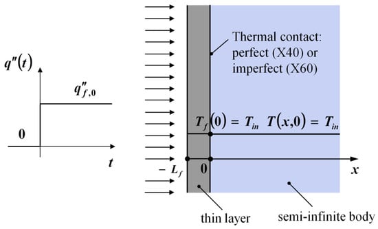
Figure 1. Schematic of the X40B1T11 problem.

The governing equations for the addressed problem, in dimensionless form, are expressed as

$$\frac{{\partial }^2\tilde{T}}{\partial {\tilde{x}}^2}=\frac{\partial \tilde{T}}{\partial \tilde{t}} (0<\tilde{x}<\infty ;\tilde{t}>0),$$

(1a)

$$-{\frac{\partial \tilde{T}}{\partial \tilde{x}}|}_{\tilde{x}=0}+P\frac{\partial {\tilde{T}}_f}{\partial \tilde{t}}=1 (\tilde{t}>0),$$

(1b)

$${\tilde{T}}_f\left(t\right)=\tilde{T}\left(0,t\right) (\tilde{t}>0),$$

(1c)

$$\tilde{T}\left(\tilde{x}\to \infty ,\tilde{t}\right)=\mathrm{finite} (\tilde{t}>0),$$

(1d)

$$\tilde{T}\left(\tilde{x},0\right)=0 (0<\tilde{x}<\infty ),$$

(1e)

$${\tilde{T}}_f\left(0\right)=0$$

(1f)

where Equation (1b,c) represent the boundary condition of the fourth kind. In particular, Equation (1b) is obtained applying the first law of thermodynamics to the thin layer; while Equation (1c) indicates a perfect contact between the semi-infinite body and the thin layer (temperature continuity).

The dimensionless variables appearing in Equation (1) are defined as

$$\tilde{T}=\frac{T-T_{in}}{{q^{″}}_{f,0}\hspace{0.17em}L/k}, {\tilde{T}}_f=\frac{T_f-T_{in}}{{q^{″}}_{f,0}\hspace{0.17em}L/k}, \tilde{x}=\frac{x}{L}, \tilde{t}=\frac{\alpha \hspace{0.17em}t}{L^2}, P=\frac{C_f{L}_f}{CL},$$

(2)

where L is a reference length, while $L_f$ is the thickness of the thin layer. Additionally, P denotes the heat capacity ratio. In dimensionless form, the problem notation becomes X40B1T00.

A well established exact analytical solution is available in the heat conduction literature ([6], p. 306, Equation (12)) for the current problem. Additionally, this solution is discussed and derived in [12], where a verified computer code is made available. It is

$$\tilde{T}\left(\tilde{x},\tilde{t}\right)=\sqrt{\frac{4\tilde{t}}{\pi }}{e}^{-\frac{{\tilde{x}}^2}{4\tilde{t}}}-\tilde{x}\mathrm{erfc}\left(\frac{\tilde{x}}{\sqrt{4\tilde{t}}}\right)-P\left[\mathrm{erfc}\left(\frac{\tilde{x}}{\sqrt{4\tilde{t}}}\right)-\mathrm{Am}\left(\tilde{x},\tilde{t},P\right)\right] (0\le \tilde{x}<\infty ;\tilde{t}\ge 0),$$

(3a)

where $\mathrm{Am}\hspace{0.17em}\left(\tilde{x},\tilde{t},P\right)$ is the so-called Amos function, defined as

$$\mathrm{Am}\left(\tilde{x},\tilde{t},P\right)=e^{\frac{\tilde{x}}{P}+\frac{\tilde{t}}{P^2}}\mathrm{erfc}\left(\frac{\tilde{x}}{\sqrt{4\tilde{t}}}+\frac{\sqrt{\tilde{t}}}{P}\right)=e^{-\frac{{\tilde{x}}^2}{4\tilde{t}}}\mathrm{erfcx}\left(\frac{\tilde{x}}{\sqrt{4\tilde{t}}}+\frac{\sqrt{\tilde{t}}}{P}\right),$$

(3b)

The $\mathrm{erfcx}\hspace{0.17em} \left(z\right)=e^{z^2}\mathrm{erfc}\hspace{0.17em} \left(z\right)$ is the scaled complementary error function. It is recommended for large values of $\tilde{x}$, $\tilde{t}$ and $1/P$ as difficulties might arise during the evaluation of Equation (3b) in its former expression because of the positive argument of the exponential term. On the contrary, the scaled complementary error function (appearing in the latter expression) approaches zero for large values of $\tilde{x}$, $\tilde{t}$ and $1/P$.

2.1. Thin Layer between Two Semi-Infinite Bodies

The solution given by Equation (3) can also be used for the three-layer configuration shown in Figure 2. In this case, a thin layer (still considered as a lumped body with temperature-independent properties) is in perfect contact with two semi-infinite bodies. The thin layer and the semi-infinite bodies are initially at uniform temperature T_in, but at t = 0 only the former is subject to a uniform and constant internal heat generation per unit of volume $g_{f,0}$.

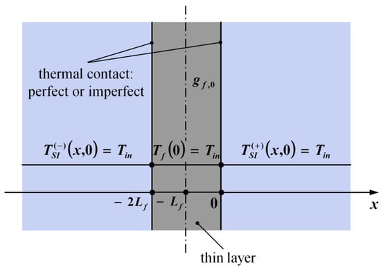
Figure 2. Three-layer structure: thin layer having 2L_f as thickness, in perfect contact with two semi-infinite bodies.

In such a case, the governing equations in dimensionless form are

$$\frac{{\partial }^2{\tilde{T}}_{SI}^{(-)}}{\partial {\tilde{x}}^2}=\frac{\partial {\tilde{T}}_{SI}^{(-)}}{\partial \tilde{t}} (-\infty <\tilde{x}<-2{\tilde{L}}_f; \tilde{t}>0),$$

(4a)

$${\tilde{T}}_{SI}^{(-)}\left(\tilde{x}\to -\infty ,\tilde{t}\right)=\mathrm{finite} (\tilde{t}>0),$$

(4b)

$${\tilde{T}}_{SI}^{(-)}\left(\tilde{x},0\right)=0 (-\infty <\tilde{x}<-2{\tilde{L}}_f),$$

(4c)

$$\frac{{\partial }^2{T}_{SI}^{(+)}}{\partial {\tilde{x}}^2}=\frac{\partial T_{SI}^{(+)}}{\partial \tilde{t}} (0<\tilde{x}<\infty ; \tilde{t}>0),$$

(4d)

$${\tilde{T}}_{SI}^{(+)}\left(\tilde{x}\to \infty ,\tilde{t}\right)=\mathrm{finite} (\tilde{t}>0),$$

(4e)

$${\tilde{T}}_{SI}^{(+)}\left(\tilde{x},0\right)=0 (0<\tilde{x}<\infty ),$$

(4f)

$$2P\frac{\partial {\tilde{T}}_f}{\partial \tilde{t}}=2+{\frac{\partial {\tilde{T}}_{SI}^{(+)}}{\partial \tilde{x}}|}_{\tilde{x}=0}-{\frac{\partial {\tilde{T}}_{SI}^{(-)}}{\partial \tilde{x}}|}_{\tilde{x}=-2{\tilde{L}}_f} (\tilde{t}>0),$$

(4g)

$${\tilde{T}}_{SI}^{(-)}\left(-2{\tilde{L}}_f,\tilde{t}\right)={\tilde{T}}_f\left(\tilde{t}\right) (\tilde{t}>0),$$

(4h)

$${\tilde{T}}_f\left(\tilde{t}\right)={\tilde{T}}_{SI}^{(+)}\left(0,\tilde{t}\right)(\tilde{t}>0),$$

(4i)

$${\tilde{T}}_f\left(0\right)=0,$$

(4j)

where Equation (4g) is obtained applying an energy balance to the thin layer; while Equation (4h,i) denote a perfect contact between the thin layer and the two semi-infinite bodies.

The dimensionless variables which appear in Equation (4) are defined as

$$\tilde{T}=\frac{T-T_{in}}{\left(g_{f,0} L_f\right)\hspace{0.17em}L/k}, {\tilde{T}}_f=\frac{T_f-T_{in}}{\left(g_{f,0} L_f\right)\hspace{0.17em}L/k}, \tilde{x}=\frac{x}{L}, \tilde{t}=\frac{\alpha \hspace{0.17em}t}{L^2}, P=\frac{C_f{L}_f}{CL}, {\tilde{L}}_f=\frac{L_f}{L},$$

(5)

For the sake of thermal symmetry, the three-layer structure depicted in Figure 2 reduces to the two-layer configuration shown in Figure 1 for perfect contact. In fact, by considering only an half-thickness of the thin layer (say $L_f$), and by noting that $\left(g_{f,0} L_f\right)$ in Equation (5) plays the same role of the surface heat flux ${q^{″}}_{f,0}$ in Equation (2), the problem defined by Equation (4) reduces to the X40B1T00 case defined by Equation (1). Hence, the thermal field ${\tilde{T}}_{SI}^{(+)}\left(\tilde{x},\tilde{t}\right)$ within the semi-infinite body on the right-side of the three-layer configuration in Figure 2 is still given by Equation (3a), which can also be used to describe the thermal field ${\tilde{T}}_{SI}^{(-)}\left(\tilde{x},\tilde{t}\right)$ on the left-side by simply replacing the variable $\tilde{x}$ with $-\left(\tilde{x}+2{\tilde{L}}_f\right)$. As far as the thin film is concerned, its temperature is defined by Equation (3a) for $\tilde{x}=0$.

3. Thin Layer in Imperfect Contact with a Semi-Infinite Body

Consider the same semi-infinite body of the problem discussed in Section 2 and shown in Figure 1, where now an imperfect thermal contact with the surface layer at the boundary x = 0 is taken into account through a contact resistance R_c. The problem notation is X60B1T11.

The governing equations, in dimensionless form, for this conductive problem are still defined by Equation (1), except the condition in Equation (1c) which has to be replaced with the following:

$$-{\frac{\partial \tilde{T}}{\partial \tilde{x}}|}_{\tilde{x}=0}=\frac{1}{{\tilde{R}}_c}\left[{\tilde{T}}_f\left(\tilde{t}\right)-\tilde{T}\left(0,\tilde{t}\right)\right] (\tilde{t}>0),$$

(6)

where ${\tilde{R}}_c=\frac{R_c}{L/k}$ is the dimensionless thermal contact resistance. Additionally, Equations (1b) and (6) represent the boundary condition of the sixth kind. In dimensionless form, the problem notation becomes X60B1T00.

3.1. Temperature Solution

To authors’ knowledge, the solution to the current problem is not available in the heat conduction literature. However, it may be obtained by applying Laplace Transform to Equations (1a,b,d) and (6), bearing in mind the initial conditions Equation (1e,f). It results in

$$\frac{{\partial }^2\vartheta }{\partial {\tilde{x}}^2}=s\vartheta (0<\tilde{x}<\infty ),$$

(7a)

$$-{\frac{\partial \vartheta }{\partial \tilde{x}}|}_{\tilde{x}=0}+Ps{\vartheta }_f=\frac{1}{s},$$

(7b)

$$\vartheta \left(\tilde{x}\to \infty ,s\right)=\mathrm{finite},$$

(7c)

$${\vartheta }_f=\vartheta \left(0,s\right)-{\tilde{R}}_c{\frac{\partial \vartheta }{\partial \tilde{x}}|}_{\tilde{x}=0},$$

(7d)

where s denotes the Laplace variable, $\vartheta \left(\tilde{x},s\right)=L\left[T\left(\tilde{x},\tilde{t}\right)\right]$, and ${\vartheta }_f\left(s\right)=L\left[{\tilde{T}}_f\left(\tilde{t}\right)\right]$.

Thus, seeking the canonical solution for Equation (7a) yields

$$\vartheta \left(\tilde{x},q\right)=c_1\exp \hspace{0.17em}\left(q \tilde{x}\right)+c_2\exp \hspace{0.17em} \left(-q \tilde{x}\right),$$

(8)

where $q=\sqrt{s}$.

The boundary condition Equation (7c) applied to Equation (8) implies $c_1=0$. Moreover, substituting Equation (7d) into Equation (7b) gives

$$-{\frac{\partial \vartheta }{\partial \tilde{x}}|}_{\tilde{x}=0}\left(1+P{\tilde{R}}_c\hspace{0.17em}s\right)+Ps\vartheta \left(0,s\right)=\frac{1}{s},$$

(9)

where $\vartheta \left(0,s\right)$ and its derivative $-{\left(\partial \vartheta /\partial \tilde{x}\right)}_{\tilde{x}=0}$ may be calculated using Equation (8). Behaving like this, the constant $c_2$ can be determined and the solution $\vartheta \left(\tilde{x},s\right)$ is

$$\vartheta \left(\tilde{x},q\right)=\frac{\exp \left(-q \tilde{x}\right)}{P{\tilde{R}}_c{q}^3\left(\frac{1}{P{\tilde{R}}_c}+\frac{q}{{\tilde{R}}_c}+q^2\right)},$$

(10)

To take the inverse of Equation (10) by means of the standard inversion tables, it is convenient to rewrite it as

$$\vartheta \left(\tilde{x},q\right)=\frac{\exp \left(-q \tilde{x}\right)}{P{\tilde{R}}_c q^3 \left(q+{\tilde{\beta }}_{ 1}\right) \left(q+{\tilde{\beta }}_{ 2}\right)},$$

(11)

where ${\tilde{\beta }}_{ 1}$ and ${\tilde{\beta }}_{ 2}$ are the roots of the polynomial appearing between round brackets at the denominator of Equation (10). They are

$${\tilde{\beta }}_{ 1}=\frac{1}{2{\tilde{R}}_c}\left(1+\sqrt{1-\frac{4{\tilde{R}}_c}{P}}\right); {\tilde{\beta }}_{ 2}=\frac{1}{2{\tilde{R}}_c}\left(1-\sqrt{1-\frac{4{\tilde{R}}_c}{P}}\right),$$

(12)

By some algebra, Equation (11) becomes

$$\begin{array}{cc}\vartheta \left(\tilde{x},q\right)& =\frac{\exp \left(-q \tilde{x}\right)}{P{\tilde{R}}_c s q \left(q+{\tilde{\beta }}_{ 1}\right) \left(q+{\tilde{\beta }}_{ 2}\right)}\frac{ \left(q+{\tilde{\beta }}_{ 2}\right)- \left(q+{\tilde{\beta }}_{ 1}\right)}{ \left({\tilde{\beta }}_{ 2}-{\tilde{\beta }}_{ 1}\right) }\\ & =\frac{{\tilde{\beta }}_{ 1} {\tilde{\beta }}_{ 2}}{ \left({\tilde{\beta }}_{ 2}-{\tilde{\beta }}_{ 1}\right)}\left[\frac{\exp \left(-q \tilde{x}\right)}{s q \left(q+{\tilde{\beta }}_{ 1}\right)}-\frac{\exp \left(-q \tilde{x}\right)}{s q \left(q+{\tilde{\beta }}_{ 2}\right)}\right]\hfill \end{array}$$

(13)

where the relation ${\tilde{\beta }}_{ 1} {\tilde{\beta }}_{ 2}=1/\left(P{\tilde{R}}_c\right)$ has been used.

Now, taking the inverse Laplace transform of Equation (13) yields

$$\tilde{T}\left(\tilde{x},\tilde{t}\right)=L^{ -1}\left[\vartheta \left(\tilde{x},q\right) \right]=\frac{{\tilde{\beta }}_{ 1} {\tilde{\beta }}_{ 2}}{ \left({\tilde{\beta }}_{ 2}-{\tilde{\beta }}_{ 1}\right)}\left\{L^{ -1}\left[\frac{\exp \left(-q \tilde{x}\right)}{ q^3 \left(q+{\tilde{\beta }}_{ 1}\right)}\right]-L^{ -1}\left[\frac{\exp \left(-q \tilde{x}\right)}{q^3 \left(q+{\tilde{\beta }}_{ 2}\right)}\right] \right\},$$

(14a)

where, by using the inversion tables provided in ([6], p. 495, Equation (15)),

$$\begin{array}{cc}{L}^{ -1}\left[\frac{\exp \left(-q \tilde{x}\right)}{s q \left(q+{\tilde{\beta }}_{ i}\right)}\right]& =\frac{1}{{\tilde{\beta }}_{ i}}\sqrt{\frac{4\tilde{t}}{\pi }}\exp \left[- {\tilde{x}}^2/\left(4\tilde{t}\right)\right]-\frac{1+{\tilde{\beta }}_{ i} \tilde{x}}{{\tilde{\beta }}_i^2}\mathrm{erfc}\left(\frac{\tilde{x}}{\sqrt{4\tilde{t}}}\right)\\ & +\frac{1}{{\tilde{\beta }}_i^2}\mathrm{Am}\left(\tilde{x},\tilde{t},1/{\tilde{\beta }}_{ i}\right)\hfill \end{array} (i = 1,2)$$

(14b)

Note that $\mathrm{Am}\left(\tilde{x},\tilde{t},1/{\tilde{\beta }}_{ i}\right)$ is the Amos function defined by Equation (3b) for $P=1/{\tilde{\beta }}_{ i}$.

Then, by substituting Equation (14b) into Equation (14a), the temperature solution is

$$\begin{array}{cc}\tilde{T}\left(\tilde{x},\tilde{t}\right)& =\sqrt{\frac{4\tilde{t}}{\pi }}\exp \left[- {\tilde{x}}^2/\left(4\tilde{t}\right)\right]-\left(P+\tilde{x}\right)\mathrm{erfc}\left(\frac{\tilde{x}}{\sqrt{4\tilde{t}}}\right)+\frac{{\tilde{\beta }}_{ 2} }{\left({\tilde{\beta }}_{ 2}-{\tilde{\beta }}_{ 1}\right) {\tilde{\beta }}_{ 1}}\mathrm{Am}\left(\tilde{x},\tilde{t},1/{\tilde{\beta }}_{ 1}\right)\\ & -\frac{{\tilde{\beta }}_{ 1} }{\left({\tilde{\beta }}_{ 2}-{\tilde{\beta }}_{ 1}\right) {\tilde{\beta }}_{ 2}}\mathrm{Am}\left(\tilde{x},\tilde{t},1/{\tilde{\beta }}_{ 2}\right)\hfill \end{array} (0\le \tilde{x}<\infty ; \tilde{t}\ge 0),$$

(15a)

Once the semi-infinite solution is known, the surface layer temperature may be determined through the boundary condition defined by Equation (6). It is

$${\tilde{T}}_f\left(\tilde{t}\right)=\sqrt{\frac{4\tilde{t}}{\pi }}-P+{\tilde{R}}_c+\frac{1 }{\left({\tilde{\beta }}_{ 2}^2-{\tilde{\beta }}_{ 1}^2\right) }\left[\frac{{\tilde{\beta }}_{ 2}^2}{{\tilde{\beta }}_{ 1}}\mathrm{Am}\left(0,\tilde{t},1/{\tilde{\beta }}_{ 1}\right)-\frac{{\tilde{\beta }}_{ 1}^2}{{\tilde{\beta }}_{ 2}}\mathrm{Am}\left(0,\tilde{t},1/{\tilde{\beta }}_{ 2}\right)\right] (\tilde{t}\ge 0),$$

(15b)

The solution given by Equation (15) is valid for any value of $\left(4{\tilde{R}}_c/P\right)$ greater than, equal or less than 1. Nevertheless, when $4{\tilde{R}}_c/P=1$, it is convenient to define the solution as follows

$$\tilde{T}\left(\tilde{x},\tilde{t}\right)=2\sqrt{\frac{4\tilde{t}}{\pi }}{e}^{-\frac{{\tilde{x}}^2}{4\tilde{t}}}-\left(P+\tilde{x}\right)\mathrm{erfc}\left(\frac{\tilde{x}}{\sqrt{4\tilde{t}}}\right)+\left(P-\tilde{x}-4\frac{\tilde{t}}{P}\right)\mathrm{Am}\left(\tilde{x},\tilde{t},P/2\right),$$

(16a)

$${\tilde{T}}_f\left(\tilde{t}\right)=\frac{3}{2}\sqrt{\frac{4\tilde{t}}{\pi }}-\frac{3}{4}P+\left(\frac{3}{4}P-2\frac{\tilde{t}}{P}\right) \mathrm{erfcx}\left(2\frac{\sqrt{\tilde{t}}}{P}\right),$$

(16b)

A verified computer code for calculating the solution of the X60B1T00 problem is provided in [13].

3.2. Thin Layer between Two Semi-Infinite Bodies: Imperfect Contact Case

The solution given by Equations (15) and (16) can also be used for the three-layer configuration shown in Figure 2 when an imperfect thermal contact between the thin layer and the semi-infinite bodies occurs. In such a case, the governing equations may still be defined by Equation (4), provided that Equation (4h,i) be replaced by the following conditions, respectively:

$${-\frac{\partial {\tilde{T}}_{SI}^{(-)}}{\partial \tilde{x}}|}_{\tilde{x}=-2{\tilde{L}}_f}=\frac{1}{{\tilde{R}}_c}\left[{\tilde{T}}_{SI}^{(-)}\left(-2{\tilde{L}}_f,\tilde{t}\right)-{\tilde{T}}_f\left(\tilde{t}\right)\right] (\tilde{t}>0),$$

(17a)

$${-\frac{\partial {\tilde{T}}_{SI}^{(+)}}{\partial \tilde{x}}|}_{\tilde{x}=0}=\frac{1}{{\tilde{R}}_c}\left[{\tilde{T}}_f\left(\tilde{t}\right)-{\tilde{T}}_{SI}^{(+)}\left(0,\tilde{t}\right)\right] (\tilde{t}>0),$$

(17b)

where the dimensionless variables are still defined by Equation (5), and ${\tilde{R}}_c=R_c/\left(L/k\right)$.

In this case, by virtue of the same considerations reported in Section 2.1, the addressed problem reduces to the X60B1T00 case. Hence, the thermal field ${\tilde{T}}_{SI}^{(+)}\left(\tilde{x},\tilde{t}\right)$ within the semi-infinite body on the right-side of the three-layer configuration is still defined by Equations (15a) and (16a). For what concerns the thermal field ${\tilde{T}}_{SI}^{(-)}\left(\tilde{x},\tilde{t}\right)$, on the left-side of Figure 2, Equations (15a) and (16a) may still be used by replacing the variable $\tilde{x}$ with $-\left(\tilde{x}+2{\tilde{L}}_f\right)$. As regards the surface layer, its temperature ${\tilde{T}}_f\left(\tilde{t}\right)$ is given by Equations (15b) and (16b).

4. Thin Layer in Perfect Contact with a Slab

Consider now a slab with temperature-independent properties, initially at uniform temperature T_in, in perfect contact with a thin layer at the boundary x = 0, and insulated at the back side as depicted in Figure 3. At $t=0$ a step change in heat flux is applied to the thin film at $x=-L_f$, which is at the same initial temperature T_in. The problem notation is X42B10T11.

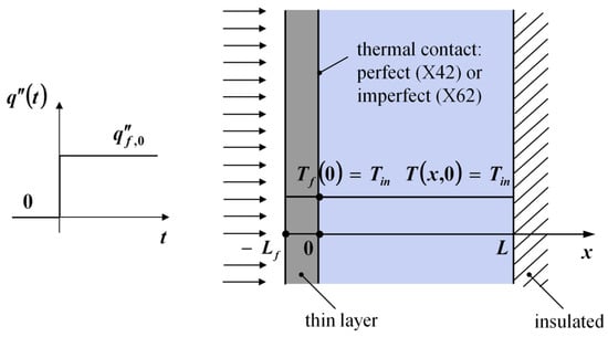
Figure 3. Schematic of the X42B10T11 problem.

The mathematical formulation of the conductive problem, in dimensionless form, is reported below.

$$\frac{{\partial }^2\tilde{T}}{\partial {\tilde{x}}^2}=\frac{\partial \tilde{T}}{\partial \tilde{t}} (0<\tilde{x}<1;\tilde{t}>0),$$

(18a)

$$-{\frac{\partial \tilde{T}}{\partial \tilde{x}}|}_{\tilde{x}=0}+P\frac{\partial {\tilde{T}}_f}{\partial \tilde{t}}=1 (\tilde{t}>0),$$

(18b)

$${\tilde{T}}_f\left(t\right)=\tilde{T}\left(0,t\right) (\tilde{t}>0),$$

(18c)

$$-{\left(\frac{\partial \tilde{T}}{\partial \tilde{x}}\right)}_{\tilde{x}=1}=0 (\tilde{t}>0),$$

(18d)

$$\tilde{T}\left(\tilde{x},0\right)=0\hspace{1em} (0<\tilde{x}<1),$$

(18e)

$${\tilde{T}}_f\left(0\right)=0,$$

(18f)

The dimensionless variable appearing in Equation (18) are defined in Equation (2), where L is now the slab thickness. In dimensionless form, the problem notation becomes X42B10T00.

The solution to the current problem may be derived by using the solution of the analogous X24B01T00 problem obtained by Carslaw and Jaeger ([6], p. 128, Equation (5)). In fact, it would be sufficient to replace the variable $\tilde{x}$ with $1-\tilde{x}$. However, as the solution method is not given in [6], a complete derivation using Green’s functions is proposed afterwards.

The Green’s function for the X42 case is available in ([4], p. 609, Equation (42)). In dimensionless form, it results in:

$${\tilde{G}}_{X42}\left(\tilde{x},\tilde{t}|{\tilde{x}}^{\prime },\tilde{\tau }\right)=\frac{1}{P+1}+2{\displaystyle \sum _{m=1}^{\infty }\frac{X_m\left(\tilde{x}\right)\hspace{0.17em}{X}_m\left({\tilde{x}}^{\prime }\right)}{{\tilde{N}}_m}\hspace{0.17em}}\exp \left[-{\beta }_m^2\left(\tilde{t}-\tilde{\tau }\right)\right],$$

(19a)

where the eigenfunction, $X_m\left(\tilde{x}\right)$, and the dimensionless norm, ${\tilde{N}}_m$ are defined as

$$X_m\left(\tilde{x}\right)=\cos \hspace{0.17em}\hspace{0.17em}\left({\beta }_m\tilde{x}\right)-P{\beta }_m\sin \hspace{0.17em}\left({\beta }_m\tilde{x}\right),$$

(19b)

$${\tilde{N}}_m={\left(P{\beta }_m\right)}^2+P+1,$$

(19c)

Additionally, the eigenvalues ${\beta }_m$ satisfy the following eigencondition

$${\beta }_m\cot ({\beta }_m)=-\frac{1}{P},$$

(19d)

whose solution is discussed in Section 4.1.

Applying the Green’s Function Solution Equation (GFSE) ([4], Chap. 6, pp. 181–182) to the current problem yields

$$\tilde{T}\left(\tilde{x},\tilde{t}\right)={\displaystyle \underset{\tilde{\tau }=0}{\overset{\tilde{t}}{\int }}{\tilde{G}}_{X42}\left(\tilde{x},\tilde{t}|0,\tilde{\tau }\right)\hspace{0.17em}d\tilde{\tau }},$$

(20)

Then, by substituting Equation (19a) into the above integral, it is found

$$\tilde{T}\left(\tilde{x},\tilde{t}\right)={\displaystyle \underset{\tilde{\tau }=0}{\overset{\tilde{t}}{\int }}\frac{1}{P+1}\hspace{0.17em}d\tilde{\tau }+2{\displaystyle \sum _{m=1}^{\infty }\frac{X_m\left(\tilde{x}\right)}{{\tilde{N}}_m}{\displaystyle \underset{\tilde{\tau }=0}{\overset{\tilde{t}}{\int }}{e}^{-{\beta }_m^2\left(\tilde{t}-\tilde{\tau }\right)}d\tilde{\tau }}}},$$

(21)

whose integration gives

$$\tilde{T}\left(\tilde{x},\tilde{t}\right)=\frac{\tilde{t}}{P+1}+2{\displaystyle \sum _{m=1}^{\infty }\hspace{0.17em}\frac{\cos \left({\beta }_m\tilde{x}\right)-P{\beta }_m\sin \left({\beta }_m\tilde{x}\right)}{{\tilde{N}}_m{\beta }_m^2}}-2{\displaystyle \sum _{m=1}^{\infty }\hspace{0.17em}\frac{\cos \left({\beta }_m\tilde{x}\right)-P{\beta }_m\left({\beta }_m\tilde{x}\right)}{{\tilde{N}}_m{\beta }_m^2}\hspace{0.17em}}\exp \left(-{\beta }_m^2\tilde{t}\right),$$

(22)

As the first summation exhibits an algebraic convergence (very slow), which requires a large number of terms, an alternative solution with better convergence properties is sought. This solution is discussed in Appendix A. Thus, by using the algebraic identity defined by Equation (A15), Equation (22) becomes

$$\begin{array}{cc}\tilde{T}\left(\tilde{x},\tilde{t}\right)& =\underset{{\tilde{T}}_s \left(\tilde{x},\tilde{t}\right)}{\underbrace{\frac{\tilde{t}}{P+1}+\frac{{\tilde{x}}^2}{2\left(P+1\right)}-\frac{\tilde{x}}{P+1}+\frac{1}{3{\left(P+1\right)}^2}}}\hspace{0.17em}\hspace{0.17em}\hspace{0.17em}\underset{{\tilde{T}}_{ct} \left(\tilde{x},\tilde{t}\right)}{\underbrace{-2{\displaystyle \sum _{m=1}^{\infty }\hspace{0.17em}\frac{\cos \left({\beta }_m\tilde{x}\right)-P{\beta }_m\sin \left({\beta }_m\tilde{x}\right)}{{\tilde{N}}_m{\beta }_m^2}\hspace{0.17em}{e}^{-{\beta }_m^2\tilde{t}}}}}\\ & \hfill (0\le \tilde{x}\le 1;\tilde{t}\ge 0),\end{array}$$

(23a)

Also, by using the interface condition defined by Equation (18c), the thin layer temperature results in

$${\tilde{T}}_f \left(\tilde{t}\right)=\underset{{\tilde{T}}_{f,s} \left(\tilde{t}\right)}{\underbrace{\frac{\tilde{t}}{P+1}+\frac{1}{3{\left(P+1\right)}^2}}}\hspace{0.17em}\hspace{0.17em}\hspace{0.17em}\underset{{\tilde{T}}_{f,ct} \left(\tilde{t}\right)}{\underbrace{-2{\displaystyle \sum _{m=1}^{\infty }\hspace{0.17em}\frac{e^{-{\beta }_m^2\tilde{t}}}{{\tilde{N}}_m{\beta }_m^2}\hspace{0.17em}}}} (\tilde{t}\ge 0),$$

(23b)

Equation (23) show two parts: a quasi-steady part, ${\tilde{T}}_s\left(\tilde{x},\tilde{t}\right)$ or ${\tilde{T}}_{f, s}\left(\tilde{t}\right)$, which yields an increasing temperature response with time, and a complementary transient part, ${\tilde{T}}_{ct}\left(\tilde{x},\tilde{t}\right)$ or ${\tilde{T}}_{f, ct}\left(\tilde{t}\right)$, which becomes negligible at large times. As regards the latter, an infinite number of terms cannot be taken into account. For this reason, a finite number of terms will be considered and the related truncation error (termed ‘tail’) is discussed in Section 4.2.

4.1. Computation of the Eigenvalues

The eigenvalues appearing in the temperature solution are computed as roots of the eigencondition defined by Equation (19d). This transcendental equation is similar to the corresponding equations of the X31 = X13 cases treated in [14]. In fact, in order to obtain Equation (19d), it is sufficient to replace the Biot number with the term 1/P. Thus, its roots (eigenvalues) may be computed by using the same explicit approximate relations based on the second-order modified Newton method [14]. These relations provide an approximate value of the exact eigenvalue with high accuracy (8-decimal place after one iteration, and 15-decimal place after two iterations) for the P range $[0\hspace{0.17em},\hspace{0.17em}\infty )$. A computer code for computing the eigenvalues of the X42 case is given in [15].

4.2. Maximum Number of Terms

The infinite summation appearing in Equation (23) exhibits an exponential convergence and, hence, very fast. A conservative convergence criterion for this summation may be defined following the procedure given in [16]. In particular, by using $\left(m-1/2\right)\pi$ as a conservative estimate for ${\beta }_m$, the maximum number of required terms $m_{\max }$ in order to get a truncation error of ${10}^{-A}$ (A = 2, 3, …, 15) in the above series solution may be taken as:

$$m_{\max }=ceil\left\{\frac{1}{2}+\frac{1}{\pi }{\left[\frac{A\ln \left(10\right)}{\tilde{t}}\right]}^{1/2}\right\},$$

(24)

where the function ‘ceil(z)’ is a Matlab function which rounds the number z to the nearest integer greater than or equal to z.

However, the criterion defined by Equation (24) may require a large number of terms for early times. To avoid it, for short times, less than the so-called deviation time ${\tilde{t}}_d$ defined as [11,17]

$${\tilde{t}}_d={\left(2-\tilde{x}\right)}^2/\left(10A\right) (A= 2, 3, \dots , 15),$$

(25)

the temperature solution Equation (23) can be replaced by the semi-infinite solution of the X40B1T00 problem, Equation (3), with an error less than ${10}^{-A}$.

Moreover, for large times, greater than the quasi-steady time ${\tilde{t}}_s$ defined by [15]

$${\tilde{t}}_s=\frac{4}{{\pi }^2}\left\{A\ln 10+\ln \left[\frac{24{\left(P+1\right)}^2}{{\pi }^2}\right]\right\},$$

(26)

the complementary transient solution of Equation (23) becomes negligible with errors less than ${10}^{-A}$ (A = 2, 3, …, 15). Thus, for $\tilde{t}\ge {\tilde{t}}_s$ the temperature solution can be taken as

$$\tilde{T}\left(\tilde{x},\tilde{t}\right)=\frac{\tilde{t}}{P+1}+\frac{{\tilde{x}}^2}{2\left(P+1\right)}-\frac{\tilde{x}}{P+1}+\frac{1}{3{\left(P+1\right)}^2} (0\le \tilde{x}\le 1;\tilde{t}\ge {\tilde{t}}_s),$$

(27)

A verified computer code in Matlab ambient for computing the solution to the X42B10T00 problem is provided in [15]. For the sake of completeness, some numerical values of ${\tilde{t}}_d$ and ${\tilde{t}}_s$ for different accuracies A are shown in Table 1.

Table 1. Deviation time and quasi-steady times for different numerical accuracies A.

A	${\tilde{\mathit{t}}}_{\mathit{d}} \left(\tilde{\mathit{x}},\mathit{A}\right)$				${\tilde{\mathit{t}}}_{\mathit{s}} \left(\mathit{P},\mathit{A}\right)$
	$\tilde{\mathit{x}}=\mathbf{0}$	$\tilde{\mathit{x}}=\mathbf{0.25}$	$\tilde{\mathit{x}}=\mathbf{0.5}$	$\tilde{\mathit{x}}=\mathbf{1}$	$\mathit{P}=\mathbf{0.01}$	$\mathit{P}=\mathbf{0.1}$	$\mathit{P}=\mathbf{1}$	$\mathit{P}=\mathbf{10}$
2	0.2000	0.1531	0.1125	0.0500	2.2346	2.3038	2.7884	4.1702
5	0.0800	0.0613	0.0450	0.0200	5.0342	5.1034	5.5880	6.9698
10	0.0400	0.0306	0.0225	0.0100	9.7002	9.7694	10.2540	11.6358
15	0.0267	0.0204	0.0150	0.0067	14.3662	14.4354	14.9200	16.3018

4.3. Thin Layer between Two Slabs

The solution defined by Equation (23) can also be used for a three-layer configuration in which a thin layer is located between two slabs insulated at the other boundaries. This situation is depicted in Figure 4, where the thin layer and the slabs are in perfect thermal contact and initially at uniform temperature T_in. At t = 0, an internal heat generation per unit of volume $g_{f,0}$ occurs only within the thin layer. For the addressed problem the governing equations are expressed as

$$\frac{{\partial }^2{\tilde{T}}_{slab}^{(-)}}{\partial {\tilde{x}}^2}=\frac{\partial {\tilde{T}}_{slab}^{(-)}}{\partial \tilde{t}} (-\left(1+2{\tilde{L}}_f\right)<\tilde{x}<-2{\tilde{L}}_f;\tilde{t}>0),$$

(28a)

$${-\frac{\partial {\tilde{T}}_{slab}^{(-)}}{\partial \tilde{x}}|}_{\tilde{x}=-\left(1+2{\tilde{L}}_f\right)}=0 (\tilde{t}>0),$$

(28b)

$${\tilde{T}}_{slab}^{(-)}\left(\tilde{x},0\right)=0\hspace{1em} (-\left(1+2{\tilde{L}}_f\right)<\tilde{x}<-2{\tilde{L}}_f),$$

(28c)

$$\frac{{\partial }^2{T}_{slab}^{(+)}}{\partial {\tilde{x}}^2}=\frac{\partial T_{slab}^{(+)}}{\partial \tilde{t}} (0<\tilde{x}<1;\tilde{t}>0),$$

(28d)

$$-{\frac{\partial {\tilde{T}}_{slab}^{(+)}}{\partial \tilde{x}}|}_{\tilde{x}=1}=0 (\tilde{t}>0),$$

(28e)

$${\tilde{T}}_{slab}^{(+)}\left(\tilde{x},0\right)=0\hspace{1em} (0<\tilde{x}<1),$$

(28f)

$$2P\frac{\partial {\tilde{T}}_f}{\partial \tilde{t}}=2+{\frac{\partial {\tilde{T}}_{slab}^{(+)}}{\partial \tilde{x}}|}_{\tilde{x}=0}-{\frac{\partial {\tilde{T}}_{slab}^{(-)}}{\partial \tilde{x}}|}_{\tilde{x}=-2{\tilde{L}}_f} (\tilde{t}>0),$$

(28g)

$${\tilde{T}}_{slab}^{(-)}\left(-2{\tilde{L}}_f,\tilde{t}\right)={\tilde{T}}_f\left(\tilde{t}\right) (\tilde{t}>0),$$

(28h)

$${\tilde{T}}_f\left(\tilde{t}\right)={\tilde{T}}_{slab}^{(+)}\left(0,\tilde{t}\right) (\tilde{t}>0),$$

(28i)

$${\tilde{T}}_f\left(0\right)=0,$$

(28j)

where Equation (28h,i) denote a perfect contact, and the dimensionless variables are defined by Equation (5).

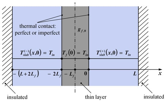
Figure 4. Three-layer structure: thin layer having 2L_f as thickness, in perfect contact with two slabs.

For the sake of thermal symmetry, the three layer structure depicted in Figure 4 reduces to the two-layer configuration shown in Figure 5 for perfect contact. Therefore, the thermal field ${\tilde{T}}_{slab}^{(+)}\left(\tilde{x},\tilde{t}\right)$ within the right slab of the three-layer configuration is still defined by Equation (23), which may also be used to describe the thermal field ${\tilde{T}}_{slab}^{(-)}\left(\tilde{x},\tilde{t}\right)$ of the left slab, by replacing the variable $\tilde{x}$ with $-\left(\tilde{x}+2{\tilde{L}}_f\right)$. As regards the thin layer, its temperature is given by Equation (23) for $\tilde{x}=0$.

It is interesting to observe that the schematic of Figure 4 represents the experimental apparatus used for thermal properties measurements [2,18]. In particular, the thin film represents the heater, while the two slabs are the specimens of the material under investigation.

5. Thin Layer in Imperfect Contact with a Slab

This problem is similar to the one discussed in Section 4 and depicted in Figure 3, but now an imperfect thermal contact with the surface layer is taken into account. Additionally, the slab and the thin layer are again at the same uniform initial temperature T_in. The problem notation is X62B10T11.

In dimensionless form, the governing equations for the current problem (whose notation becomes X62B10T00) are still defined by Equation (18), except the interface condition, Equation (18c), which has to be replaced with Equation (6).

The exact analytical solution to the current X62B10T00 problem is available in the heat conduction literature ([6], p. 129, Equation (14)). However, as in this reference the solution method is not given, a complete derivation using Laplace transform is proposed afterwards. Contrary to the X42 case treated in Section 4.2, the GF approach cannot here be used as the $G_{X62}\left(\tilde{x},\tilde{t}|{\tilde{x}}^{\prime },\tilde{\tau }\right)$ Green’s function is not available in the literature.

By applying the Laplace transform to Equations (18a,b,d) and (6), subject to the initial conditions, Equation (18e,f), it results in the same problem defined by Equation (7), where now Equation (7c) valid for a semi-infinite body has to be replaced with an insulating condition, that is,

$${\left(\frac{\partial \vartheta }{\partial \tilde{x}}\right)}_{\tilde{x}=1}=0,$$

(29)

where $\vartheta \left(\tilde{x},s\right)=L\left[\tilde{T}\left(\tilde{x},\tilde{t}\right)\right]$.

In the current case however, it is convenient to rewrite the solution given by Equation (8) by using a linear combinations of exponentials, such as $\left(e^{q\tilde{x}}-e^{-q\tilde{x}}\right)/2$ and $\left(e^{q\tilde{x}}+e^{-q\tilde{x}}\right)/2$. Thus, Equation (8) becomes

$$\vartheta \left(\tilde{x},q\right)=B_{ 1}\cosh \left(q\tilde{x}\right)+B_{ 2}\sinh \left(q\tilde{x}\right)=A\cosh \left(q\tilde{x}+\varphi \right),$$

(30)

where $q=\sqrt{s}$ and the phase $\varphi$ can be determined by applying the boundary condition at $\tilde{x}=1$, i.e., Equation (29). It follows that: $\varphi =-q$. Then, as the hyperbolic cosine is an even function, Equation (30) becomes

$$\vartheta \left(\tilde{x},q\right)=A\cosh \left[q\left(\tilde{x}-1\right)\right]=A\cosh \left[q\left(1-\tilde{x}\right)\right],$$

(31)

Also, by using the boundary condition of the sixth kind defined by Equation (7b,d) in the Laplace domain, it is possible to determine the constant A as

$$A=\frac{1}{P{q}^4\cosh \left(q\right)+q{ }^3\left(P{\tilde{R}}_c q^2+1\right)\hspace{0.17em}\sinh \left(q\right)},$$

(32)

Thus, the sought solution $\vartheta \left(\tilde{x},q\right)$ is

$$\vartheta \left(\tilde{x},q\right)=\frac{\cosh \left[q\left(1-\tilde{x}\right)\right]}{\underset{D\left(q\right)}{\underbrace{q^2\left[P{q}^2\cosh \left(q\right)+q\left(P{\tilde{R}}_c q^2+1\right)\hspace{0.17em}\sinh \left(q\right)\right]}}}=\frac{\cosh \left[q\left(1-\tilde{x}\right)\right]}{D\left(q\right)},$$

(33)

To take the inverse of Equation (33) a Taylor series expansion of the hyperbolic functions is needed. It results in

$$\cosh \left[q\left(1-\tilde{x}\right)\right]=1+\frac{q^2\left(1-\tilde{x}\right)}{2}+O\left(q^4\right),$$

(34a)

$$\cosh \left(q\right)=1+\frac{q^2}{2}+O\left(q^4\right),$$

(34b)

$$\sinh \left(q\right)=q+\frac{q^3}{3!}+O\left(q^5\right),$$

(34c)

Therefore, the function $D\left(q\right)$ at the denominator of Equation (33) becomes

$$\begin{array}{cc}D\left(q\right)& =q^2\left\{P{q}^2\left[1+\frac{q^2}{2}+O\left(q^4\right)\right]+q\left(P{\tilde{R}}_c q^2+1\right)\hspace{0.17em}\left[q+\frac{q^3}{3!}+O\left(q^5\right)\right]\right\}\hfill \\ & =q^4\left\{P+1+q^2\left[\frac{P}{2}+P{\tilde{R}}_c+\frac{1}{6}\right]+O\left(q^4\right)\right\}\hfill \end{array}$$

(35)

The above function admits a quadruple pole at q = 0 (which implies a double pole at s = 0). Additionally, it has simple zeros along the negative real axis, that may conveniently be assumed as $q=i\beta$ (or $s=-{\beta }^2$). Then, the value of $\beta$ can be computed by solving numerically the eigencondition $D\left(q=i\beta \right)=0$, that is

$$P\beta \cos \left(\beta \right)+\left(1-P{\tilde{R}}_c {\beta }^2\right)\hspace{0.17em}\sin \left(\beta \right)=0,$$

(36)

where the relations $\cosh \hspace{0.17em}\left(i\beta \right)=\cos \hspace{0.17em}\left(\beta \right)$ and $\sinh \hspace{0.17em}\left(i\beta \right)=i\sin \hspace{0.17em}\left(\beta \right)$ have been used. Equation (36) admits an infinite number of simple poles at $q=i{\beta }_m$,${\beta }_m>0$, m = 1, 2, … (or $s=-{\beta }_m^2$), where ${\beta }_m$ is the m-th eigenvalue whose computation is discussed in Section 5.1.

Since the function $\vartheta \left(\tilde{x},q\right)$ in Equation (33) is analytic except at poles q = 0 (s = 0) and at poles $q=i{\beta }_m$ ($s=-{\beta }_m^2$), ${\beta }_m>0$, m = 1, 2, …, the inverse of such a function may be obtained using the residue theorem ([19], pp. 384–385).

$$\begin{array}{ll}\tilde{T}\left(\tilde{x},\tilde{t}\right)=L^{-1}\left\{\vartheta \left(\tilde{x},s\right)\right\}=\frac{1}{2\pi i}{\displaystyle \underset{\gamma -i\infty }{\overset{\gamma +i\infty }{\int }}\vartheta \left(\tilde{x},s\right) e^{st}ds}& ={\sum }_{ \mathrm{Residues}\hspace{0.17em}\mathrm{in}\hspace{0.17em}\mathrm{the}\hspace{0.17em}\mathrm{closed}\hspace{0.17em}\mathrm{contour}\hspace{0.17em} }^{ \mathrm{encompassing}\hspace{0.17em}\mathrm{the}\hspace{0.17em}\mathrm{left}\hspace{0.17em}\mathrm{half}\hspace{0.17em}\mathrm{plane}}\hfill \\ & =R_{s=0}+{\displaystyle \sum _{m=1}^{\infty }{R}_{s=-{\beta }_m^2}}\hfill \end{array}$$

(37)

where the calculation of the residues, $R_{s=0}$ and $R_{s=-{\beta }_m^2}$, is given in Appendix B. In particular, they result in

$$R_{s=0}=\frac{\tilde{t}}{P+1}+\frac{{\tilde{x}}^2}{2\left(P+1\right)}-\frac{\tilde{x}}{P+1}+\frac{1-3P{\tilde{R}}_c}{3{\left(P+1\right)}^2},$$

(38a)

$$R_{s=-{\beta }_m^2}=\frac{2 \left(P{\tilde{R}}_c{\beta }_m^2-1\right)\cos \left[{\beta }_m\left(1-\tilde{x}\right)\right]\hspace{0.17em}{e}^{-{\beta }_m^2\hspace{0.17em}\tilde{t}}}{\left[{\left(P{\tilde{R}}_c\right)}^2{\beta }_m^4+\left(P+P{\tilde{R}}_c-2{\tilde{R}}_c\right)P{\beta }_m^2+P+1\right]\hspace{0.17em}{\beta }_m^2\cos \left({\beta }_m\right)},$$

(38b)

Substituting Equation (38a,b) in Equation (37) yields the temperature solution in the time domain.

$$\begin{array}{cc}\tilde{T}\left(\tilde{x},\tilde{t}\right)& =\underset{{\tilde{T}}_s\left(\tilde{x},\tilde{t}\right)}{\underbrace{\frac{\tilde{t}}{P+1}+\frac{{\tilde{x}}^2}{2\left(P+1\right)}-\frac{\tilde{x}}{P+1}+\frac{1-3P{\tilde{R}}_c}{3{\left(P+1\right)}^2}}}\hspace{0.17em}\hspace{0.17em}\underset{{\tilde{T}}_{ct}\left(\tilde{x},\tilde{t}\right)}{\underbrace{+2{\displaystyle \sum _{m=1}^{\infty }\hspace{0.17em}\frac{\left(P{\tilde{R}}_c{\beta }_m^2-1\right)\cos \left[{\beta }_m\left(1-\tilde{x}\right)\right]}{{\tilde{N}}_m{\beta }_m^2\cos \left({\beta }_m\right)}\hspace{0.17em}{e}^{-{\beta }_m^2\tilde{t}}}}}\\ & \hfill (0\le \tilde{x}\le 1;\tilde{t}\ge 0),\end{array}$$

(39a)

where ${\tilde{N}}_m$ is the dimensionless norm given by

$${\tilde{N}}_m={\left(P{\tilde{R}}_c\right)}^2{\beta }_m^4+\left(P+P{\tilde{R}}_c-2{\tilde{R}}_c\right)P{\beta }_m^2+P+1,$$

(39b)

Once $\tilde{T}\left(\tilde{x},\tilde{t}\right)$ is known, the thin layer temperature ${\tilde{T}}_f\left(\tilde{t}\right)$ may be obtained by using the boundary condition defined by Equation (6). After some algebra, it is given by

$${\tilde{T}}_f\left(\tilde{t}\right)=\underset{{\tilde{T}}_{f,s}\left( \tilde{t}\right)}{\underbrace{\frac{\tilde{t}}{P+1}+\frac{{\tilde{R}}_c+1/3}{{\left(P+1\right)}^2}}}\hspace{0.17em}\hspace{0.17em}\underset{{\tilde{T}}_{f,ct}\left( \tilde{t}\right)}{\underbrace{-2{\displaystyle \sum _{m=1}^{\infty }\frac{e^{-{\beta }_m^2\tilde{t}}}{{\tilde{N}}_m{\beta }_m^2}\hspace{0.17em}}}} (\tilde{t}\ge 0),$$

(39c)

Similarly to the X42B10T00 case, the temperature solutions given by Equation (39a,c) show two components: a quasi-steady part and a complementary transient part that becomes negligible at large times. The maximum number of terms and the truncation error of the sums in Equation (39a,c) will be analyzed in Section 5.2.

5.1. Computation of the Eigenvalues

The X62 eigencondition defined by Equation (36) may be rewritten as

$$\tan ({\beta }_m)=\frac{\frac{{\beta }_m}{{\tilde{R}}_c}}{{\beta }_m^{ 2}-\frac{1}{P{\tilde{R}}_c}},$$

(40)

This transcendental equation is similar to the corresponding equation of the X33 case approached in [14]. In detail, it is needed to replace the sum of the Biot numbers $\left(B_{\hspace{0.17em}1}+B_{\hspace{0.17em}2}\right)$ with the term $1/{\tilde{R}}_c$, and their product $\left(B_{\hspace{0.17em}1}{B}_{\hspace{0.17em}2}\right)$ with the term $1/\left(P{\tilde{R}}_c\right)$. Therefore, its roots (eigenvalues) may be computed by using the same explicit approximate relations based on the third-order modified Newton method [14]. These relations provide an approximate value ${\zeta }_m$ of the exact eigenvalue ${\beta }_m$ (m = 1, 2, 3, …), with at least seven-decimal place accuracy (10⁻⁷) for $P\in \left(0,\infty \right)$ and for ${\tilde{R}}_c\in \left(0,\infty \right)$. Additionally, the lowest accuracy of 10⁻⁷ occurs when m = 1; on the contrary, when m > 1, the accuracy is higher [14]. A computer code for computing the eigenvalues of the X62 case is given in Ref. [20].

5.2. Computational Solution

The exact analytical solution given by Equation (39) shows an infinite summation, while the computational analytical solution requires a finite number of terms. In particular, the maximum number of required terms $m_{\max }$ for a truncation error less than ${10}^{-A}$ (A = 2, 3, …, 15), may be taken in a conservative way as [20]:

$$m_{\max }=1+\mathrm{ceil}\left\{\frac{1}{\pi }\sqrt{\frac{A\ln \left(10\right)+\hspace{0.17em}\left[H\left(P-1\right)-1\right]\ln \left(P\right)}{\tilde{t}}}\right\},$$

(41)

where $H(\cdot )$ denotes the Heaviside step function.

As the convergence criterion defined by Equation (41) may require a large number of terms for early times, the solution of the X62B10T00 problem can be replaced by the semi-infinite transient X60B1T00 solution given by Equations (15) and (16). In fact, at early times the finite body behaves as a semi-infinite one. In particular, for times less than the so-called deviation time ${\tilde{t}}_d$ defined by Equation (25), this replacement occurs with errors with less than ${10}^{-A}$ [11,17].

Moreover, for time greater than the so-called steady time ${\tilde{t}}_s$, the complementary transient part of the solution defined by Equation (39a,c) may be neglected with errors less than ${10}^{-A}$. Therefore,

$$\tilde{T}\left(\tilde{x},\tilde{t}\right)=\frac{\tilde{t}}{P+1}+\frac{{\tilde{x}}^2}{2\left(P+1\right)}-\frac{\tilde{x}}{P+1}+\frac{1-3P{\tilde{R}}_c}{3{\left(P+1\right)}^2} (0\le \tilde{x}\le 1;\tilde{t}\ge {\tilde{t}}_s),$$

(42a)

$${\tilde{T}}_f\left(\tilde{t}\right)=\frac{\tilde{t}}{P+1}+\frac{{\tilde{R}}_c+1/3}{{\left(P+1\right)}^2} (\tilde{t}\ge {\tilde{t}}_s),$$

(42b)

where ${\tilde{t}}_s$ may be taken in a conservative way as [20]

$${\tilde{t}}_s=\frac{A^{\left(1+2/A\right)}\ln 10+\hspace{0.17em}\left[H\left({\tilde{N}}_1 {\beta }_1^2-1\right)-1\right]\ln \left({\tilde{N}}_1 {\beta }_1^2\right)}{{\beta }_1^2},$$

(43)

Some numerical values of ${\tilde{t}}_s$ for different accuracies A are shown in Table 2. Additionally, a verified computer code in Matlab ambient for computing the solution of the X62B10T00 problem is provided in [20].

Table 2. Quasi-steady times for several P and ${\tilde{R}}_c$ values and two different accuracies A.

P	$\mathit{A}=\mathbf{2}$			$\mathit{A}=\mathbf{10}$
	${\tilde{\mathit{R}}}_{\mathit{c}}=\mathbf{0.01}$	${\tilde{\mathit{R}}}_{\mathit{c}}=\mathbf{0.1}$	${\tilde{\mathit{R}}}_{\mathit{c}}=\mathbf{1}$	${\tilde{\mathit{R}}}_{\mathit{c}}=\mathbf{0.01}$	${\tilde{\mathit{R}}}_{\mathit{c}}=\mathbf{0.1}$	${\tilde{\mathit{R}}}_{\mathit{c}}=\mathbf{1}$
0.01	0.9520	0.9521	0.9540	3.7719	3.7726	3.7798
0.1	1.1254	1.1405	1.4396	4.4591	4.5190	5.7040
1	2.2681	2.5609	6.3138	8.9868	10.1470	25.0168
10	3.5249	4.1530	11.3281	13.9664	16.4553	44.8845

5.3. Thin Layer between Two Slabs: Imperfect Contact Case

The solution given by Equation (39) may also be used for the three-layer configuration shown in Figure 4 when an imperfect thermal contact between the slabs and the thin layer is taken into account.

The related governing equations may still be defined by Equation (28), provided that Equation (28h,i) be replaced by the following interface conditions, respectively:

$${-\frac{\partial {\tilde{T}}_{slab}^{(-)}}{\partial \tilde{x}}|}_{\tilde{x}=-2{\tilde{L}}_f}=\frac{1}{{\tilde{R}}_c}\left[{\tilde{T}}_{slab}^{(-)}\left(-2{\tilde{L}}_f,\tilde{t}\right)-{\tilde{T}}_f\left(\tilde{t}\right)\right] (\tilde{t}>0),$$

(44a)

$${-\frac{\partial {\tilde{T}}_{slab}^{(+)}}{\partial \tilde{x}}|}_{\tilde{x}=0}=\frac{1}{{\tilde{R}}_c}\left[{\tilde{T}}_f\left(\tilde{t}\right)-{\tilde{T}}_{slab}^{(+)}\left(0,\tilde{t}\right)\right] (\tilde{t}>0),$$

(44b)

With the same argumentations reported in Section 4.3 the addressed problem reduces to the X62B10T00 case. Hence, the thermal field within the right slab, in the three-layer configuration, is still defined by Equation (41a). It may also be used to describe the thermal field ${\tilde{T}}_{slab}^{(-)}\left(\tilde{x},\tilde{t}\right)$, developing in the left slab, by replacing the variable $\tilde{x}$ with $-\left(\tilde{x}+2{\tilde{L}}_f\right)$. For what concerns the thin layer, its temperature ${\tilde{T}}_f\left(\tilde{t}\right)$ is still given by Equation (39c).

It has already been mentioned in Section 4.3 that the schematic of Figure 4 finds application in the field of thermal properties measurements when using transient inverse techniques. In such an application, the contact resistance ${\tilde{R}}_c$ accounts for the imperfect contact between the heater (thin layer) and the specimens (slabs) [21].

6. Results and Discussion

6.1. Thin Layer in Perfect Contact with a Semi-Infinite Body

Figure 5a shows the dimensionless temperature for the X40B1T00 problem as a function of $\tilde{x}$ and for different $\tilde{t}$ values, while Figure 5b depicts the dimensionless temperature for the same case as a function of $\tilde{t}$ and for different dimensionless locations $\tilde{x}$. Both figures are obtained for P = 1. Note that in Figure 5b the curve for $\tilde{x}=0$ also represents the thin layer temperature ${\tilde{T}}_f\left(\tilde{t}\right)$.

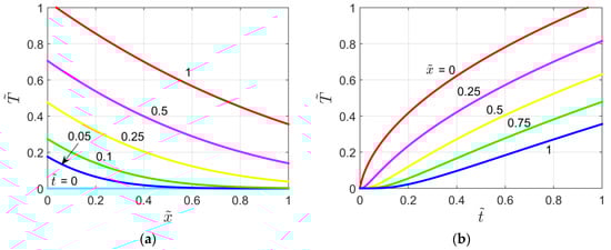
Figure 5. Dimensionless temperature plots for the X40B1T00 problem: (a) Temperature vs. $\tilde{x}$ and $\tilde{t}$ as a parameter; (b) Temperature vs. $\tilde{t}$ and $\tilde{x}$ as a parameter.

Figure 6 shows the temperature distribution within the semi-infinite medium for different values of the heat capacity ratio P and for $\tilde{t}=0.2$. As shown by the figure the temperature reached in the medium decreases when the P parameter rises. Additionally, it is interesting to observe that for $P\to 0$ the X40B1T00 problem reduces to the case of a semi-infinite body subject to a jump in heat flux (X20B1T0 case [22]).

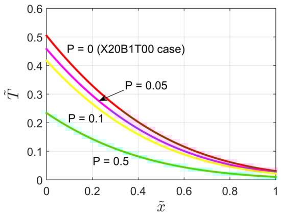
Figure 6. Dimensionless temperature distribution for the X40B1T00 problem for different values of the heat capacity ratio.

6.2. Thin Layer in Imperfect Contact with a Semi-Infinite Body

Figure 7a,b depict the dimensionless temperature for the X60B1T00 problem as a function of dimensionless space and time $\tilde{t}$, respectively (for P = 1 and ${\tilde{R}}_c=0.25$). Moreover, in Figure 7b the thin layer temperature ${\tilde{T}}_f\left(\tilde{t}\right)$ is also plotted.

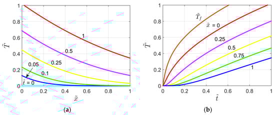
Figure 7. Dimensionless temperature plots for the X60B1T00 problem: (a) Temperature vs. $\tilde{x}$ and $\tilde{t}$ as a parameter; (b) Temperature vs. $\tilde{t}$ and $\tilde{x}$ as a parameter.

A comparison between Figure 5 and Figure 7 exhibits that the temperature reached for the X60B1T00 problem (imperfect thermal contact case) is slightly lower than that obtained when the perfect contact at the thin layer/semi-infinite body interface is considered (X40B1T00 problem).

Figure 8 displays the temperature distribution within the semi-infinite body for different values of the dimensionless contact resistance ${\tilde{R}}_c$, for P = 0.1 and $\tilde{t}=0.2$. It can be observed that the temperature field decreases when the contact resistance increases. However, the temperature at $\tilde{x}=1$ is less affected by the ${\tilde{R}}_c$ parameter. Note that for ${\tilde{R}}_c\to 0$ the X60B1T00 problem simply reduces to the X40B1T00 problem treated in Section 2.

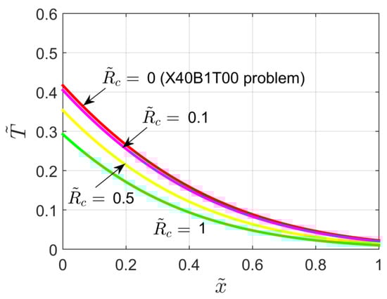
Figure 8. Dimensionless temperature distribution for the X60B1T00 problem for different values of the dimensionless contact resistance.

6.3. Thin Layer in Perfect Contact with a Slab

The dimensionless temperature field within the slab of the X42B10T00 problem (P = 1) is plotted as a function of $\tilde{x}$ in Figure 9a, and as a function of time in Figure 9b. Note that in Figure 9b the curve for $\tilde{x}=0$ also represents the thin layer temperature ${\tilde{T}}_f\left(\tilde{t}\right)$.

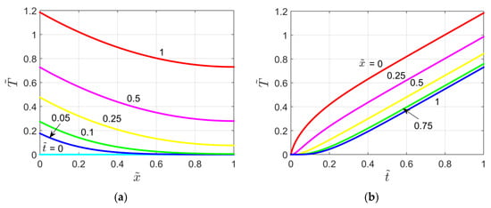
Figure 9. Dimensionless temperature plots for the X42B10T00 problem: (a) Temperature vs. $\tilde{x}$ and $\tilde{t}$ as a parameter; (b) Temperature vs. $\tilde{t}$ and $\tilde{x}$ as a parameter.

By using the thickness of the slab L as a reference length for the semi-infinite body, it is possible to compare the results obtained for the X40B1T00 (Figure 5) and X42B10T00 (Figure 9) problems. Therefore, a comparison between Figure 5 and Figure 9 gives evidence that the temperature distribution within the finite slab is greater than that obtained for the semi-infinite body (not for times less than the deviation time). However, for small values of $\tilde{x}$ this difference is more visible at large $\tilde{t}$ values, while for large values of $\tilde{x}$ it can be observed also for shorter times.

The influence of the heat capacity ratio P on the temperature distribution occurring within the slab is shown by Figure 10. A behavior similar to that displayed by Figure 6 can be observed. Note that for $P\to 0$ the X42B10T00 problem reduces to the case of a finite slab subject to a jump in heat flux (X22B10T0 case [23]).

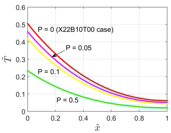
Figure 10. Dimensionless temperature distribution for the X42B10T00 problem for different values of the heat capacity ratio ($\tilde{t}=0.2$).

6.4. Thin Layer in Imperfect Contact with a Slab

Figure 11 shows a plot of the dimensionless temperature as a function of $\tilde{x}$ for different time values (Figure 11a), and as a function of $\tilde{t}$ for different locations (Figure 11b). Additionally, the thin layer temperature ${\tilde{T}}_f\left(\tilde{t}\right)$ is depicted in Figure 11b.

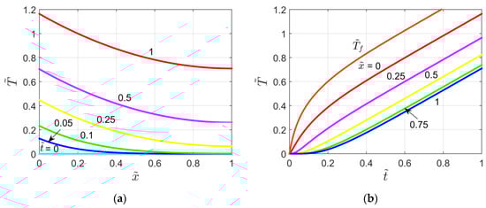
Figure 11. Dimensionless temperature plots for the X62B10T00 problem: (a) Temperature vs. $\tilde{x}$ and $\tilde{t}$ as a parameter; (b) Temperature vs. $\tilde{t}$ and $\tilde{x}$ as a parameter (P = 1 and ${\tilde{R}}_c=0.25$).

By comparing Figure 9 (perfect contact case) and Figure 11 it is possible to state that the temperature field obtained for a slab in imperfect contact with a thin layer is slightly lower than that occurring when a perfect contact is considered (X42B10T00 problem).

Also, with the same argumentation reported in the previous Subsection, Figure 7 (X60B1T00 problem) and Figure 11 are compared. By observing these figures it is clear that the finite thickness of the slab yields a temperature distribution greater than that obtained in a semi-infinite body in imperfect contact with a thin layer (Figure 7). This behavior is more evident for large time values and occurs also for the thin layer temperature.

Finally, the influence of the contact resistance ${\tilde{R}}_c$ on the temperature distribution within the slab (at $\tilde{t}=0.2$) is shown by Figure 12. Similarly to what has been discussed for Figure 8, when the contact resistance increases, lower temperature values are obtained. Note that for ${\tilde{R}}_c\to 0$ the X62B10T00 problem simply reduces to the X42B10T00 problem discussed in Section 5.

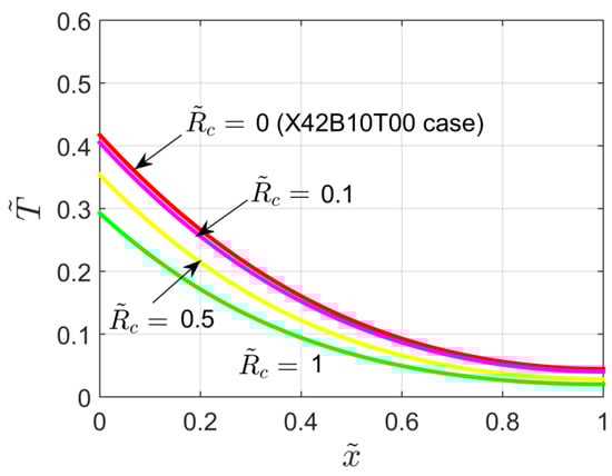
Figure 12. Dimensionless temperature distribution for the X62B10T00 problem for different values of the dimensionless contact resistance and P = 0.1.

7. Conclusions

One-dimensional multi-layer transient heat conduction problems involving boundary conditions of fourth and sixth kind have been discussed.

In particular, structures in which a thin layer and a semi-infinite body are in perfect or imperfect thermal contact (X40B1T00 and X60B1T00 problems, respectively) have been investigated. Additionally in these situations a jump in the heat flux was applied to the thin layer. Furthermore, the temperature solution of the X60B1T00 problem, which is not available in the heat conduction literature, has been derived by means of the LT method.

Two-layer problems defined by a thin layer in perfect or imperfect thermal contact with a slab, insulated at the other boundary, have also been investigated. In particular, the exact analytical solutions for the X42B10T00 and X62B10T00 problems have been derived by means of the GFSE and the LT methods, respectively.

Moreover situations in which a thin layer, with internal heat generation, is located between two adjacent domains (semi-infinite bodies or slabs) have been discussed. For sake of thermal symmetry occurring in one dimensional conductive problems, such three-layer structures have been reduced to the two-layer configurations previously analyzed.

The results have been shown that for all the considered cases the temperature levels reached in the domain increase when the heat capacity of the thin layer and the contact resistance at the thin layer-domain interface decrease. In particular, the greatest temperature field has been obtained for a finite body in perfect thermal contact with a thin layer. Additionally, when an imperfect contact is considered, it has been found that the thin layer temperature is highest when the adjacent domain is a slab and it increases when the contact resistance rises.

References

- Van der Tempel, L.; Potze, W.; Lammers, J.H. Transient heat conduction in a thin layer between semi-infinite media in polymer shaping. J. Heat Transf. 2018, 140, 041301. [Google Scholar] [CrossRef]
- D’Alessandro, G.; de Monte, F. Optimal experiment design for thermal property estimation using a boundary condition of the fourth kind with a time-limited heating period. Int. J. Heat Mass Transf. 2019, 134, 1268–1282. [Google Scholar] [CrossRef]
- Carr, E.J.; Wood, C.J. Rear-surface integral method for calculating thermal diffusivity: Finite pulse time correction and two-layer samples. Int. J. Heat Mass Transf. 2019, 144, 118609. [Google Scholar] [CrossRef]
- Cole, K.D.; Beck, J.V.; Haji-Sheikh, A.; Litkouhi, B. Heat Conduction Using Green’s Function, 2nd ed.; CRC Press Taylor & Francis: Boca Raton, FL, USA, 2011. [Google Scholar]
- Al-Nimr, M.A.; Alkam, M.K. A generalized thermal boundary condition. Heat Mass Transf. 1997, 33, 157–161. [Google Scholar] [CrossRef]
- Carslaw, H.S.; Jaeger, J.C. Conduction of Heat in Solids, 2nd ed.; Oxford University Press: New York, NY, USA, 1959. [Google Scholar]
- Deconinck, B.; Pelloni, B.; Sheils, N.E. Non-steady-state heat conduction in composite walls. Proc. R. Soc. A 2014, 470, 20130605. [Google Scholar] [CrossRef] [PubMed]
- Rodrigo, M.R.; Worthy, A.L. Solution of multilayer diffusion problems via the Laplace transform. J. Math. Anal. Appl. 2016, 444, 475–502. [Google Scholar] [CrossRef]
- Van der Tempel, L. Temperature solution for transient heat conduction in a thin bilayer between semi-infinite media in thermal effusivity measurement. J. Heat Transf. 2016, 138, 051301. [Google Scholar] [CrossRef]
- Zhou, L.; Bai, M.; Cui, W.; Lü, J. Theoretical solution of transient heat conduction problem in one-dimensional multilayer composite media. J. Thermophys. Heat Transf. 2017, 31, 483–488. [Google Scholar] [CrossRef]
- Cole, K.D.; Beck, J.V.; Woodbury, A.; de Monte, F. Intrinsic verification and a heat conduction database. Int. J. Therm. Sci. 2014, 78, 36–47. [Google Scholar] [CrossRef]
- De Monte, F.; Beck, J.V. X40B1T00, Exact Analytical Conduction Toolbox. October 2013, pp. 1–18. Available online: www.exact.unl.edu (accessed on 1 October 2020).
- Giacchetti, L.; de Monte, F. X60B1T00, Exact Analytical Conduction Toolbox. September 2015, pp. 1–72. Available online: www.exact.unl.edu (accessed on 1 October 2020).
- Haji-Sheikh, A.; Beck, J.V. An efficient method of computing eigenvalues in heat conduction. Numer. Heat Transf. Part B Fundam. 2000, 38, 133–156. [Google Scholar] [CrossRef]
- D’Alessandro, G.; de Monte, F. X42B10T00, Exact Analytical Conduction Toolbox. July 2016, pp. 1–73. Available online: www.exact.unl.edu (accessed on 1 October 2020).
- De Monte, F.; Beck, J.V.; Amos, D.E. A heat-flux based building block approach for solving heat conduction problems. Int. J. Heat Mass Transf. 2011, 54, 2789–2800. [Google Scholar] [CrossRef]
- De Monte, F.; Beck, J.V.; Amos, D.E. Solving two-dimensional Cartesian unsteady heat conduction problems for small values of the time. Int. J. Therm. Sci. 2012, 60, 106–113. [Google Scholar] [CrossRef]
- D’Alessandro, G.; de Monte, F. Sensitivity coefficients for thermal properties measurements using a boundary condition of the 4th kind. J. Phys. Conf. Ser. 2017, 796, 012011. [Google Scholar] [CrossRef]
- Arpaci, V.S. Conduction Heat Transfer; Addison-Wesley Publishing Company: Ann Arbor, MI, USA, 1966. [Google Scholar]
- D’Alessandro, G.; de Monte, F.; Amos, D. X62B10T00, Exact Analytical Conduction Toolbox. February 2017, pp. 1–95. Available online: www.exact.unl.edu (accessed on 1 October 2020).
- D’Alessandro, G.; de Monte, F. On the optimum experiment and heating times when estimating thermal properties through the plane source method. Heat Transf. Eng. 2021, 43. in press. [Google Scholar]
- De Monte, F.; Beck, J.V. X20B1T0, Exact Analytical Conduction Toolbox. January 2013, pp. 1–12. Available online: www.exact.unl.edu (accessed on 30 November 2020).
- De Monte, F.; Beck, J.V. X22B10T0, Exact Analytical Conduction Toolbox. February 2013, pp. 1–14. Available online: www.exact.unl.edu (accessed on 30 November 2020).
Publisher’s Note: MDPI stays neutral with regard to jurisdictional claims in published maps and institutional affiliations. |
© 2020 by the authors. Licensee MDPI, Basel, Switzerland. This article is an open access article distributed under the terms and conditions of the Creative Commons Attribution (CC BY) license (http://creativecommons.org/licenses/by/4.0/).