Grid Code-Dependent Frequency Control Optimization in Multi-Terminal DC Networks


 ,
, 
 ,
,  and
and 
Abstract
1. Introduction
2. Frequency Related Grid Code Requirements
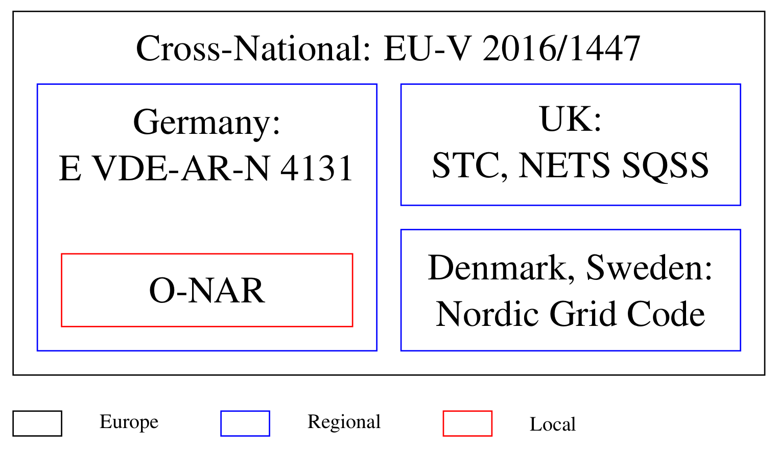
2.1. Regulation Levels
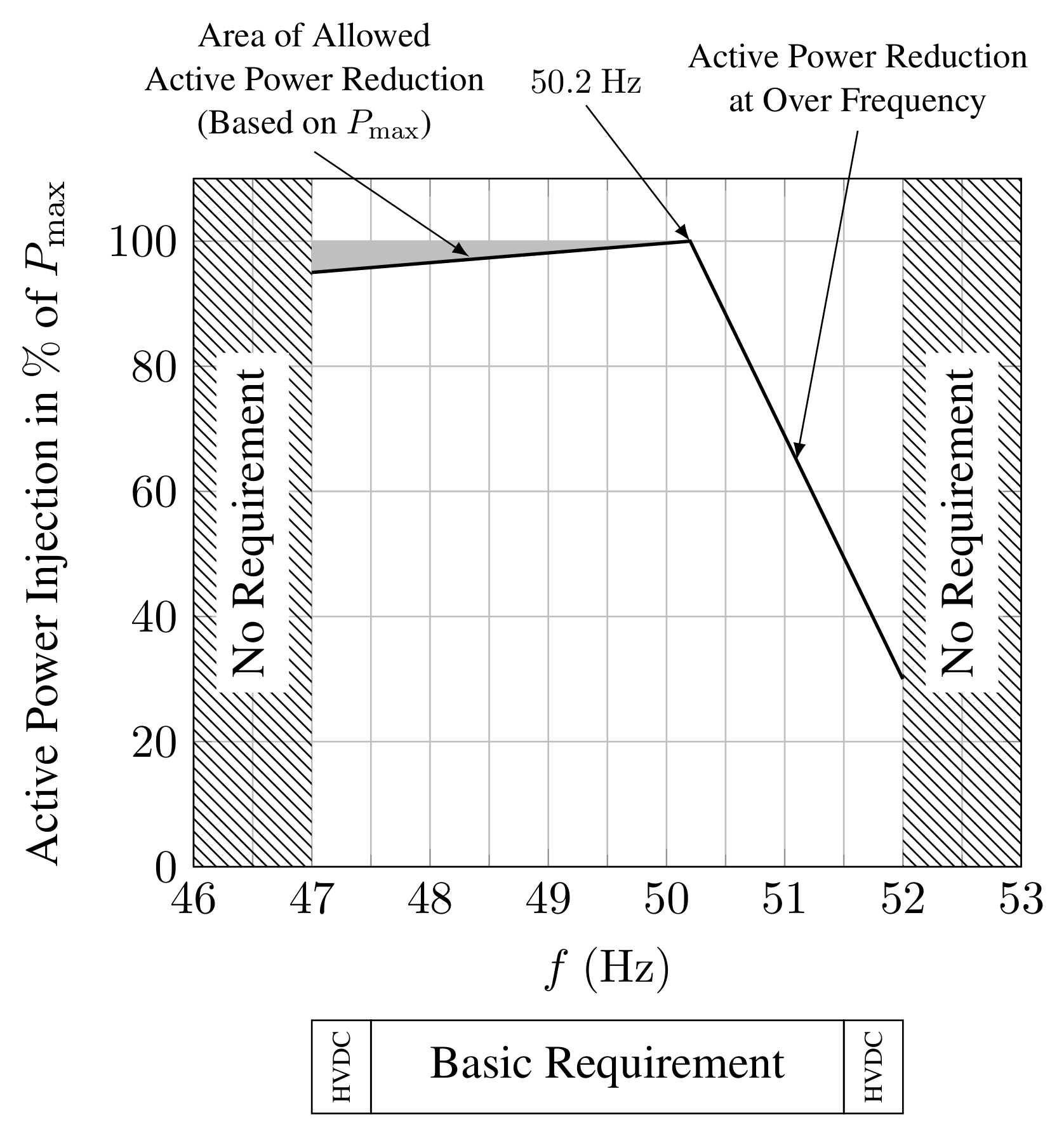
2.2. Requirements for Power Plants Connected to HVDC Systems
- 50 Hz (49 Hz to 51 Hz) for of the week;
- 50 Hz ( to Hz) of the time.
2.3. Synthetic Inertia
2.4. Requirements from Grid Codes
3. HVDC Modeling
3.1. AC System Dynamics
3.2. Converter and MTDC System Dynamics
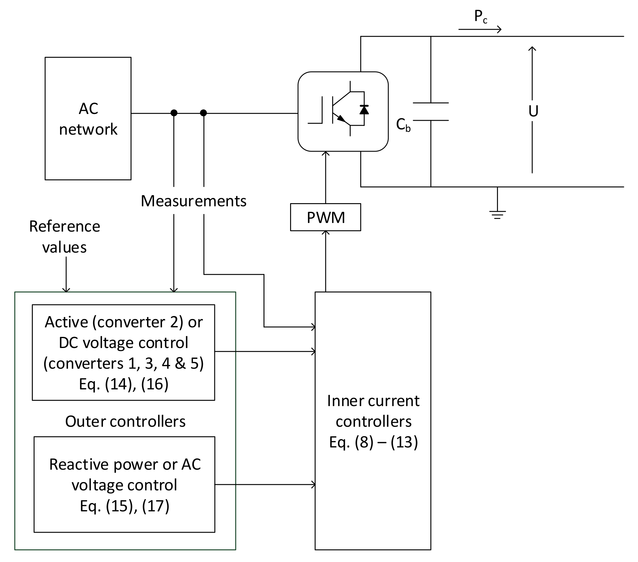
3.3. Converter Control
3.4. Droop Control
3.5. Phase-Locked Loop
4. Proposed Controller
4.1. Optimal Performance Indicators
4.2. Controller Optimization Using Particle Swarm Optimization
4.3. Python-PSCAD Interface
5. Results and Discussion
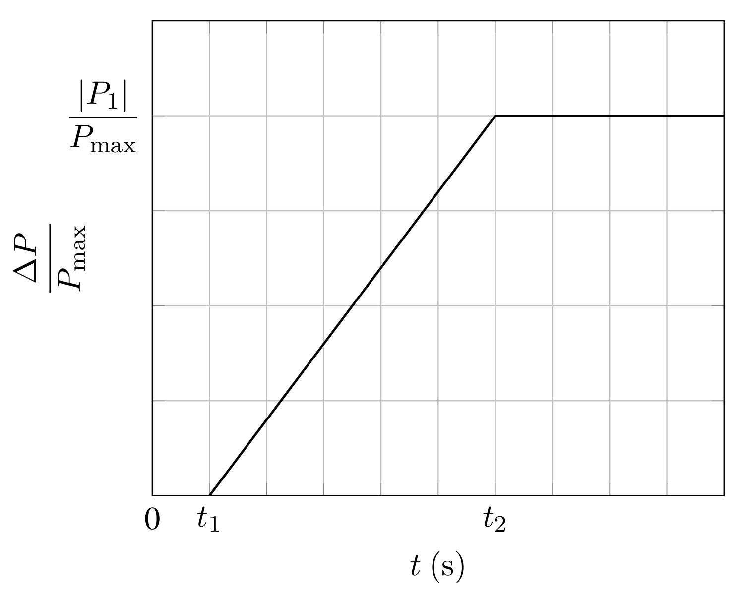
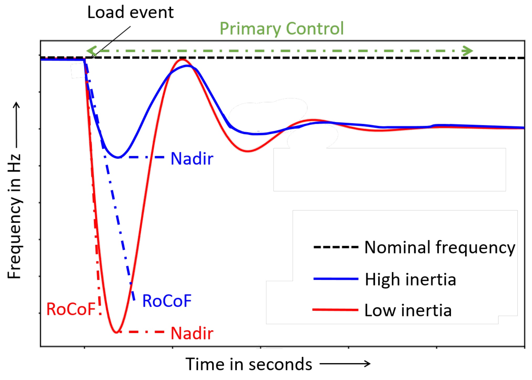
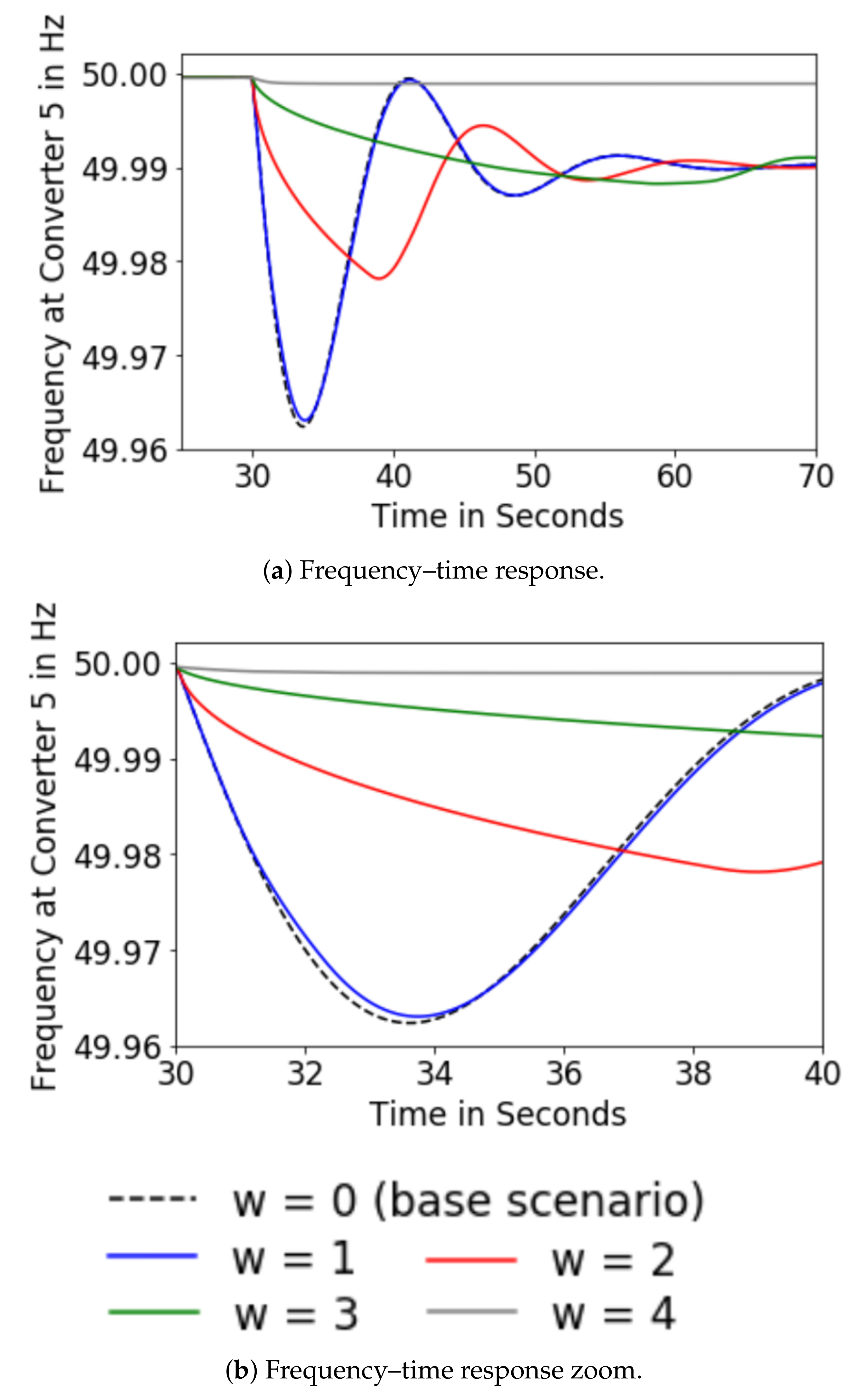
- The should not be very steep according to the grid code requirements. If the is too steep, the converters would disconnect from the AC grid and could therefore no longer support it, thus provoking power imbalances;
- The should not drop below a specific value to ensure that the converter stays connected to the grid and follows the grid code limits;
- The settling time needs to be minimized to reach a stable operating state as quickly as possible, as an earlier recovery means less impact.
5.1. Base Case Scenario
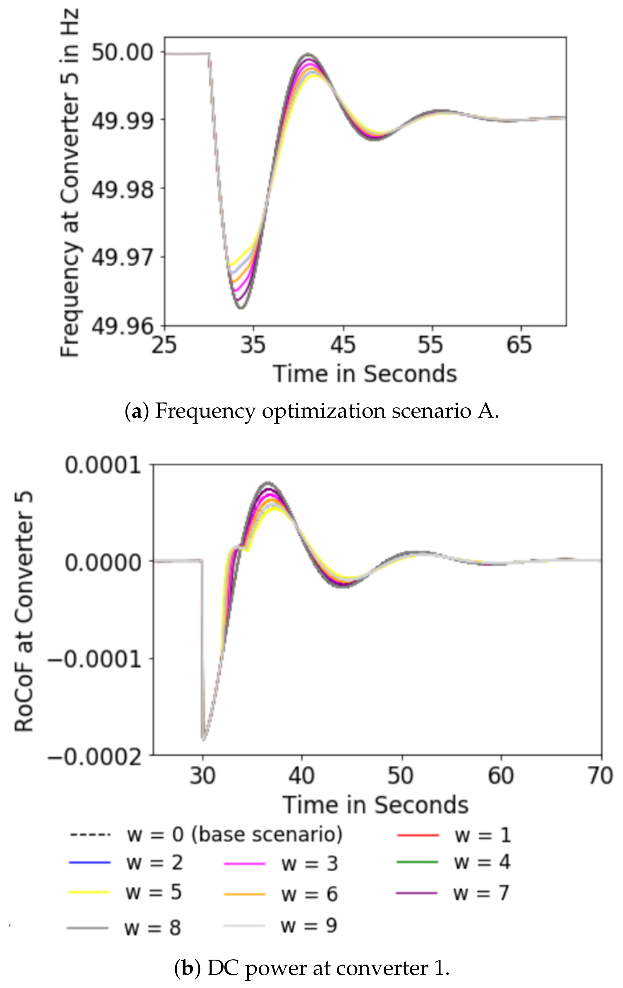
5.2. Scenario A
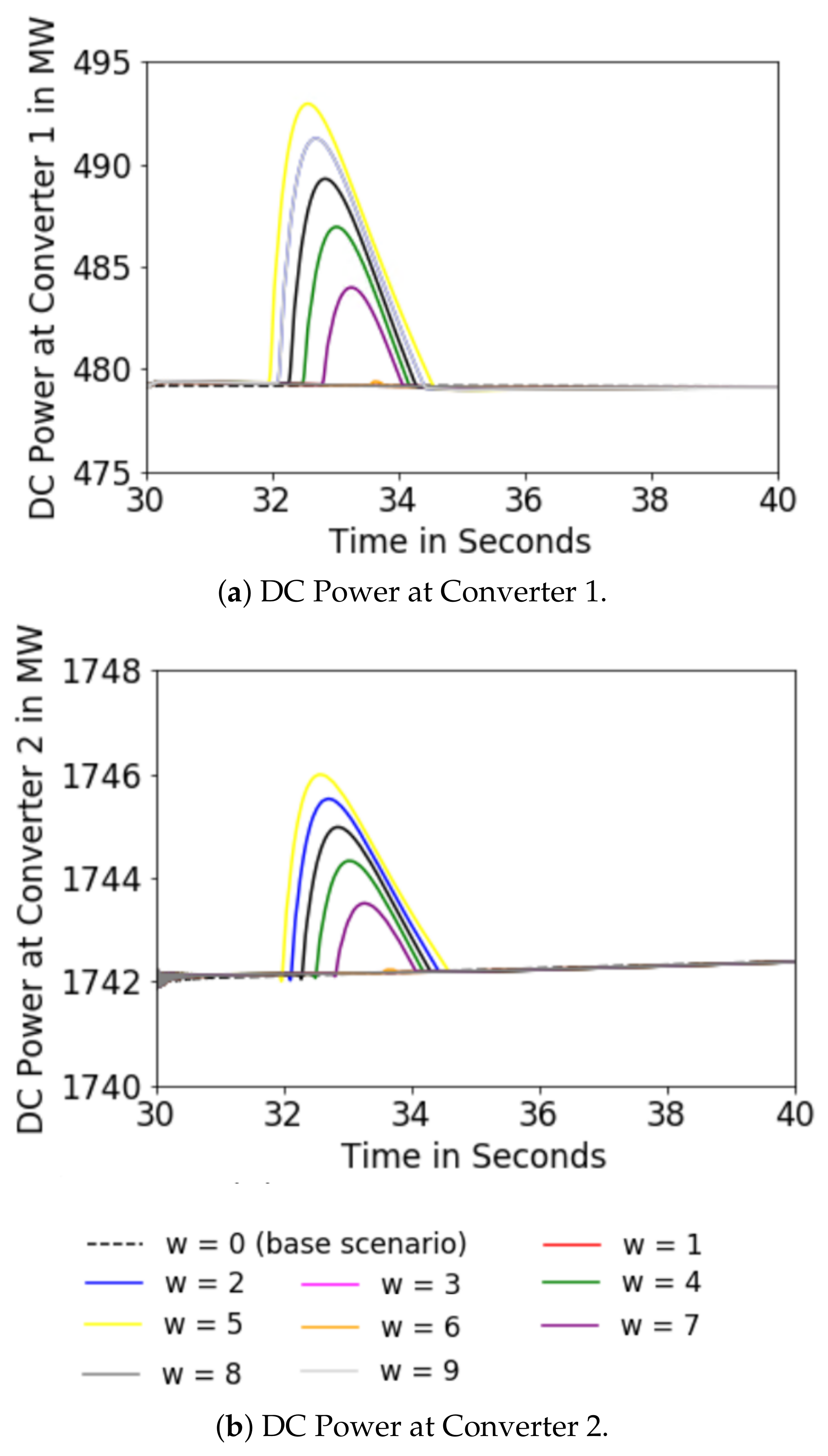
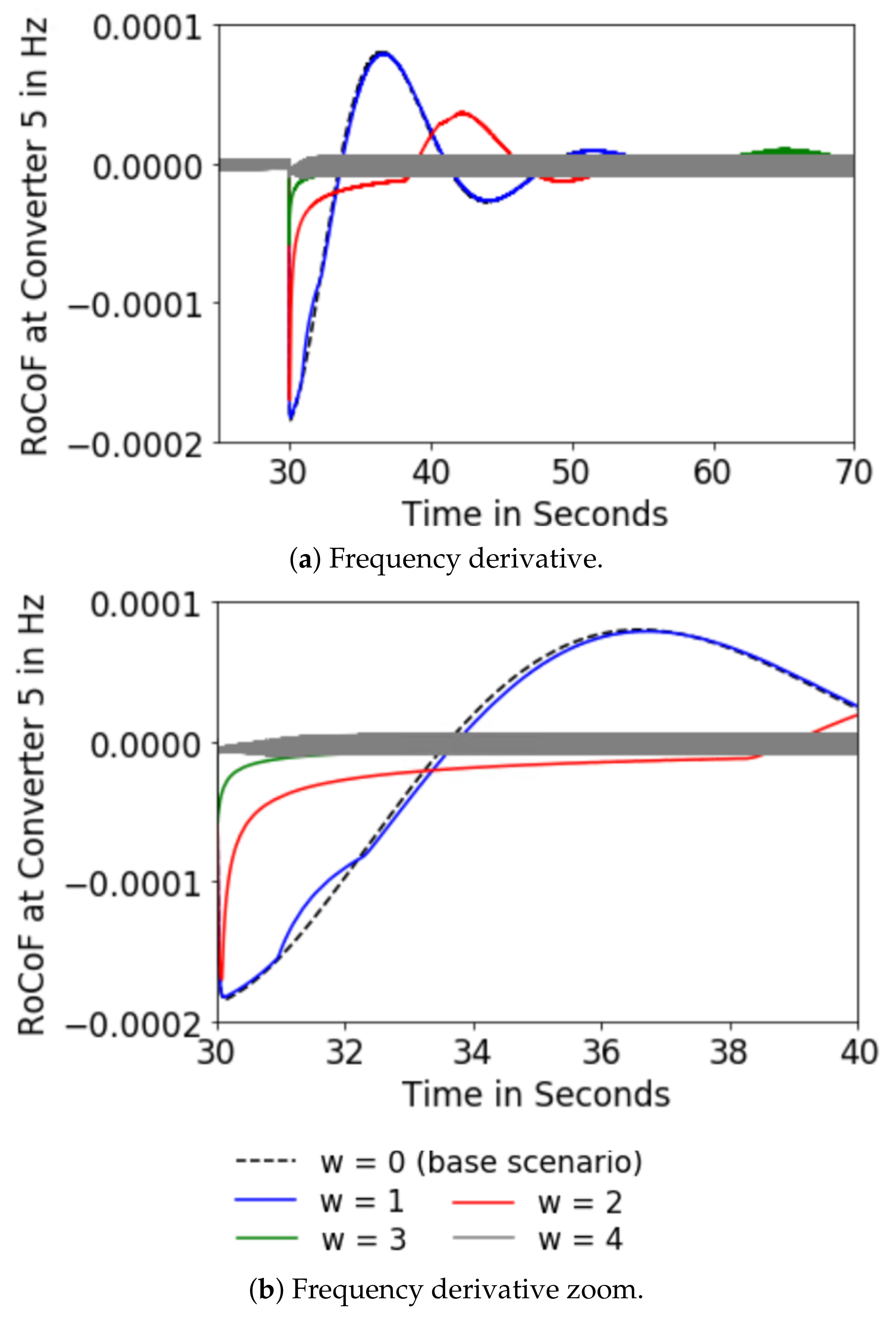
5.3. Scenario B
6. Conclusions
Author Contributions
Funding
Conflicts of Interest
References
- Strbac, G.; Konstantinidis, C.V.; Moreno, R.; Konstantelos, I.; Papadaskalopoulos, D. It’s All About Grids: The Importance of Transmission Pricing and Investment Coordination in Integrating Renewables. IEEE Power Energy Mag. 2015, 13, 61–75. [Google Scholar] [CrossRef]
- Chamorro, H.R.; Ordonez, C.A.; Peng, J.C.; Ghandhari, M. Non-synchronous generation impact on power systems coherency. IET Gener. Trans. Distrib. 2016, 10, 2443–2453. [Google Scholar] [CrossRef]
- Milano, F.; Dörfler, F.; Hug, G.; Hill, D.J.; Verbič, G. Foundations and Challenges of Low-Inertia Systems (Invited Paper). In Proceedings of the 2018 Power Systems Computation Conference (PSCC), Dublin, Ireland, 11–15 June 2018; pp. 1–25. [Google Scholar] [CrossRef]
- Liu, X.; Lindemann, A. Control of VSC-HVDC Connected Offshore Windfarms for Providing Synthetic Inertia. IEEE J. Emerg. Select. Top. Power Electr. 2018, 6, 1407–1417. [Google Scholar] [CrossRef]
- Cao, J.; Du, W.; Wang, H.F.; Bu, S.Q. Minimization of Transmission Loss in Meshed AC/DC Grids with VSC-MTDC Networks. IEEE Trans. Power Syst. 2013, 28, 3047–3055. [Google Scholar] [CrossRef]
- Ordonez, C.A.; Puentes, A.; Chamorro, H.R.; Ramos, G. p-q theory for active compensation applied to supergrids and microgrids. In Proceedings of the 2012 Workshop on Engineering Applications, Bogota, Colombia, 2–4 May 2012; pp. 1–6. [Google Scholar] [CrossRef]
- Chamorro, H.R.; Ramos, G. Harmonic and power flow hybrid controller applied to VSC based HVDC stations. In Proceedings of the 2010 IEEE/PES Transmission and Distribution Conference and Exposition: Latin America (T D-LA), Sao Paulo, Brazil, 8–10 November 2010; pp. 245–250. [Google Scholar] [CrossRef]
- Litzenberger, W.; Mitsch, K.; Bhuiyan, M. When It’s Time to Upgrade: HVdc and FACTS Renovation in the Western Power System. IEEE Power Energy Mag. 2016, 14, 32–41. [Google Scholar] [CrossRef]
- Yuan, Z.; You, S.; Liu, Y.; Liu, Y.; Osborn, D.; Pan, J. Frequency control capability of Vsc-Hvdc for large power systems. In Proceedings of the 2017 IEEE Power Energy Society General Meeting, Birmingham, UK, 10–12 February 2017; pp. 1–5. [Google Scholar]
- Zhou, H.; Su, Y.; Chen, Y.; Ma, Q.; Mo, W. The China Southern Power Grid: Solutions to Operation Risks and Planning Challenges. IEEE Power Energy Mag. 2016, 14, 72–78. [Google Scholar] [CrossRef]
- Gemmell, B.; Korytowski, M. Refurbishments in Australasia: Upgrades of HVdc in New Zealand and FACTS in Australia. IEEE Power Energy Mag. 2016, 14, 72–79. [Google Scholar] [CrossRef]
- Kim, S.; Kim, H.; Lee, H.; Lee, J.; Lee, B.; Jang, G.; Lan, X.; Kim, T.; Jeon, D.; Kim, Y.; et al. Expanding Power Systems in the Republic of Korea: Feasibility Studies and Future Challenges. IEEE Power Energy Mag. 2019, 17, 61–72. [Google Scholar] [CrossRef]
- Irnawan, R.; Da Silva, F.F.; Bak, C.L.; Bregnhøj, T.C. An initial topology of multi-terminal HVDC transmission system in Europe: A case study of the North-Sea region. In Proceedings of the 2016 IEEE International Energy Conference (ENERGYCON), Leuven, Belgium, 4–8 April 2016; pp. 1–6. [Google Scholar] [CrossRef]
- Pan, J.; Callavik, M.; Lundberg, P.; Zhang, L. A Subtransmission Metropolitan Power Grid: Using High-Voltage dc for Enhancement and Modernization. IEEE Power Energy Mag. 2019, 17, 94–102. [Google Scholar] [CrossRef]
- Chamorro, H.R.; Riaño, I.; Gerndt, R.; Zelinka, I.; Gonzalez-Longatt, F.; Sood, V.K. Synthetic Inertia Control Based on Fuzzy Adaptive Differential Evolution. Int. J. Electr. Power Energy Syst. 2019, 105, 803–813. [Google Scholar] [CrossRef]
- Zhang, W.; Rouzbehi, K.; Luna, A.; Gharehpetian, G.B.; Rodriguez, P. Multi-terminal HVDC grids with inertia mimicry capability. IET Renew. Power Gener. 2016, 10, 752–760. [Google Scholar] [CrossRef]
- Andreasson, M.; Dimarogonas, D.V.; Sandberg, H.; Johansson, K.H. Distributed Controllers for Multiterminal HVDC Transmission Systems. IEEE Trans. Control Netw. Syst. 2017, 4, 564–574. [Google Scholar] [CrossRef]
- McNamara, P.; Milano, F. Model Predictive Control-Based AGC for Multi-Terminal HVDC-Connected AC grids. IEEE Trans. Power Syst. 2018, 33, 1036–1048. [Google Scholar] [CrossRef]
- Zhu, J.; Booth, C.D.; Adam, G.P.; Roscoe, A.J.; Bright, C.G. Inertia Emulation Control Strategy for VSC-HVDC Transmission Systems. IEEE Trans. Power Syst. 2013, 28, 1277–1287. [Google Scholar] [CrossRef]
- Zhu, J.; Guerrero, J.M.; Hung, W.; Booth, C.D.; Adam, G.P. Generic inertia emulation controller for multi-terminal voltage-source-converter high voltage direct current systems. IET Renew. Power Gener. 2014, 8, 740–748. [Google Scholar] [CrossRef]
- Ndreko, M.; Bucurenciu, A.; Popov, M.; Van der Meijden, M.A.M.M. On grid code compliance of offshore mtdc grids: Modeling and analysis. In Proceedings of the 2015 IEEE Eindhoven PowerTech, Eindhoven, The Netherlands, 29 June–2 July 2015; pp. 1–6. [Google Scholar] [CrossRef]
- Ye, Y.; Lu, Z.; Xie, L.; Qiao, Y. A Coordinated Frequency Regulation Strategy for VSC-HVDC Integrated Offshore Wind Farms. In Proceedings of the 2018 IEEE Power Energy Society General Meeting (PESGM), Portland, OR, USA, 5–10 August 2018; pp. 1–5. [Google Scholar]
- Papangelis, L.; Guillaud, X.; Cutsem, T.V. Frequency support among asynchronous AC systems through VSCs emulating power plants. In Proceedings of the 11th IET International Conference on AC and DC Power Transmission, Birmingham, UK, 10–12 February 2015; pp. 1–9. [Google Scholar]
- Jose, K.; Adeuyi, O.; Liang, J.; Ugalde-Loo, C.E. Coordination of fast frequency support from multi-terminal HVDC grids. In Proceedings of the 2018 IEEE International Energy Conference (ENERGYCON), Limassol, Cyprus, 3–7 June 2018; pp. 1–6. [Google Scholar]
- Kirakosyan, A.; El-Saadany, E.F.; El Moursi, M.S.; Salama, M. Selective Frequency Support Approach for MTDC Systems Integrating Wind Generation. IEEE Trans. Power Syst. 2020. [Google Scholar] [CrossRef]
- Zhang, Q.; McCalley, J.D.; Ajjarapu, V.; Renedo, J.; Elizondo, M.; Tbaileh, A.; Mohan, N. Primary Frequency Support through North American Continental HVDC Interconnections with VSC-MTDC Systems. IEEE Trans. Power Syst. 2020. [Google Scholar] [CrossRef]
- Adeuyi, O.D.; Cheah-Mane, M.; Liang, J.; Jenkins, N. Fast Frequency Response From Offshore Multiterminal VSC–HVDC Schemes. IEEE Trans. Power Deliv. 2017, 32, 2442–2452. [Google Scholar] [CrossRef]
- Ai, Q.; Liu, T.; Yin, Y.; Tao, Y. Frequency coordinated control strategy of HVDC sending system with wind power based on situation awareness. IET Gener. Trans. Distrib. 2020, 14, 3179–3186. [Google Scholar] [CrossRef]
- Xiong, Y.; Yao, W.; Wen, J.; Lin, S.; Ai, X.; Fang, J.; Wen, J.; Cheng, S. Two-Level Combined Control Scheme of VSC-MTDC Integrated Offshore Wind Farms for Onshore System Frequency Support. IEEE Trans. Power Syst. 2020. [Google Scholar] [CrossRef]
- Rouzbehi, K.; Miranian, A.; Luna, A.; Rodriguez, P. Optimized control of multi-terminal DC GridsUsing particle swarm optimization. In Proceedings of the 2013 15th European Conference on Power Electronics and Applications (EPE), Lille, France, 3–5 September 2013; pp. 1–9. [Google Scholar] [CrossRef]
- Namara, P.M.; Meere, R.; O’Donnell, T.; McLoone, S. Distributed MPC for Frequency Regulation in Multi-Terminal HVDC Grids. IFAC Proc. Vol. 2014, 47, 11141–11146. [Google Scholar] [CrossRef]
- Wen, Y.; Zhan, J.; Chung, C.Y.; Li, W. Frequency Stability Enhancement of Integrated AC/VSC-MTDC Systems With Massive Infeed of Offshore Wind Generation. IEEE Trans. Power Syst. 2018, 33, 5135–5146. [Google Scholar] [CrossRef]
- Papangelis, L.; Debry, M.; Panciatici, P.; Van Cutsem, T. Coordinated Supervisory Control of Multi-Terminal HVDC Grids: A Model Predictive Control Approach. IEEE Trans. Power Syst. 2017, 32, 4673–4683. [Google Scholar] [CrossRef]
- Raza, A.; Yousaf, Z.; Jamil, M.; Gilani, S.O.; Abbas, G.; Uzair, M.; Shaheen, S.; Benrabah, A.; Li, F. Multi-Objective Optimization of VSC Stations in Multi-Terminal VSC-HVdc Grids, Based on PSO. IEEE Access 2018, 6, 62995–63004. [Google Scholar] [CrossRef]
- Gonzalez-Longatt, F.M.; Acosta, M.N.; Chamorro, H.R.; Torres, J.L.R. Power Converters Dominated Power Systems; Springer: Cham, Switzerland, 2021; pp. 1–35. [Google Scholar] [CrossRef]
- COMMISSION REGULATION (EU) 2016/ 1447—of 26 August 2016—Establishing a Network Code on Requirements for Grid Connection of High Voltage Direct Current Systems and Direct Current-Connected Power Park Modules. p. 65. Available online: https://eur-lex.europa.eu/eli/reg/2016/1447/oj (accessed on 4 December 2020).
- Saborío-Romano, O. Connection of OWPPs to HVDC Networks Using VSCs and Diode Rectifiers: An Overview. p. 5. Available online: https://www.researchgate.net/publication/322571208_Connection_of_OWPPs_to_HVDC_networks_using_VSCs_and_Diode_Rectifiers_an_Overview (accessed on 4 December 2020).
- VDE/FNN. Technische Anschlussregeln für HGÜ-Systeme und über HGÜ-Systeme Angeschlossene Erzeugungsanlagen. Available online: https://www.vde.com/de/fnn/arbeitsgebiete/tar/tar-hgue (accessed on 4 December 2020).
- Winter, W.; Chan, D.; Norton, M.; Haesen, E.; Székely, Á. Towards a european network code for HVDC connections and offshore wind integration. In Proceedings of the 2015 50th International Universities Power Engineering Conference (UPEC), Stoke on Trent, UK, 1–4 September 2015; pp. 1–6. [Google Scholar]
- GmbH., T.T. Offshore-Netzanschlussregeln—O-NAR. 2017. Available online: https://docplayer.org/56149134-Offshore-netzanschlussregeln-o-nar-tennet-tso-gmbh.html (accessed on 4 December 2020).
- Rate of Change of Frequency (RoCoF) Withstand Capability—ENTSO-E Guidance Document for National Implementation for Network Codes on Grid Connection. Available online: https://eepublicdownloads.entsoe.eu/clean-documents/Network%20codes%20documents/NC%20RfG/IGD_RoCoF_withstand_capability_final.pdf (accessed on 7 December 2020).
- Need for Synthetic Inertia (SI) for Frequency Regulation—ENTSO-E Guidance Document for National Implementation for Network Codes on Grid Connection. Available online: https://eepublicdownloads.entsoe.eu/clean-documents/Network%20codes%20documents/NC%20RfG/IGD_Need_for_Synthetic_Inertia_final.pdf (accessed on 7 December 2020).
- Chamorro, H.R.; Sanchez, A.C.; Verjordet, A.; Jimenez, F.; Gonzalez-Longatt, F.; Member, S.; Sood, V.K. Distributed Synthetic Inertia Control in Power Systems. In Proceedings of the 8th International Conference on Energy and Environment: Energy Saved Today is Asset for Future, CIEM 2017, Bucharest, Romania, 19–20 October 2017; pp. 74–78. [Google Scholar] [CrossRef]
- Chuquen, R.M.; Chamorro, H.R. Graph Theory Applications to Deregulated Power Systems; Springer Briefs in Electrical and Computer Engineering; Springer International Publishing: Berlin, Germany, 2021. [Google Scholar] [CrossRef]
- Saad, H.; Peralta, J.; Dennetiere, S.; Mahseredjian, J.; Jatskevich, J.; Martinez, J.A.; Davoudi, A.; Saeedifard, M.; Sood, V.; Wang, X.; et al. Dynamic Averaged and Simplified Models for MMC-Based HVDC Transmission Systems. IEEE Trans. Power Deliv. 2013, 28, 1723–1730. [Google Scholar] [CrossRef]
- Cole, S.; Beerten, J.; Belmans, R. Generalized Dynamic VSC MTDC Model for Power System Stability Studies. IEEE Trans. Power Syst. 2010, 25, 1655–1662. [Google Scholar] [CrossRef]
- Haileselassie, T.M. Control, Dynamics and Operation of Multi-terminal VSC-HVDC Transmission Systems. 2012. Available online: https://ntnuopen.ntnu.no/ntnu-xmlui/handle/11250/257409 (accessed on 4 December 2020).
- Fahad, S.; Mahdi, A.J.; Tang, W.H.; Huang, K.; Liu, Y. Particle Swarm Optimization Based DC-Link Voltage Control for Two Stage Grid Connected PV Inverter. In Proceedings of the 2018 International Conference on Power System Technology (POWERCON), Guangzhou, China, 6–8 November 2018; pp. 2233–2241. [Google Scholar]


| Parameter | Value Range |
|---|---|
| 1.5–10% | |
| TSO | |
| Iteration w | Settling Time (s) | Nadir (Hz) |
|---|---|---|
| = 2 | ||
| = 3 | ||
| = 4 | ||
| = 5 | ||
| = 6 | ||
| = 7 | ||
| = 8 | ||
| = 9 |
Publisher’s Note: MDPI stays neutral with regard to jurisdictional claims in published maps and institutional affiliations. |
© 2020 by the authors. Licensee MDPI, Basel, Switzerland. This article is an open access article distributed under the terms and conditions of the Creative Commons Attribution (CC BY) license (http://creativecommons.org/licenses/by/4.0/).
Share and Cite
Hoffmann, M.; Chamorro, H.R.; Lotz, M.R.; Maestre, J.M.; Rouzbehi, K.; Gonzalez-Longatt, F.; Kurrat, M.; Alvarado-Barrios, L.; Sood, V.K. Grid Code-Dependent Frequency Control Optimization in Multi-Terminal DC Networks. Energies 2020, 13, 6485. https://doi.org/10.3390/en13246485
Hoffmann M, Chamorro HR, Lotz MR, Maestre JM, Rouzbehi K, Gonzalez-Longatt F, Kurrat M, Alvarado-Barrios L, Sood VK. Grid Code-Dependent Frequency Control Optimization in Multi-Terminal DC Networks. Energies. 2020; 13(24):6485. https://doi.org/10.3390/en13246485
Chicago/Turabian StyleHoffmann, Melanie, Harold R. Chamorro, Marc René Lotz, José M. Maestre, Kumars Rouzbehi, Francisco Gonzalez-Longatt, Michael Kurrat, Lazaro Alvarado-Barrios, and Vijay K. Sood. 2020. "Grid Code-Dependent Frequency Control Optimization in Multi-Terminal DC Networks" Energies 13, no. 24: 6485. https://doi.org/10.3390/en13246485
APA StyleHoffmann, M., Chamorro, H. R., Lotz, M. R., Maestre, J. M., Rouzbehi, K., Gonzalez-Longatt, F., Kurrat, M., Alvarado-Barrios, L., & Sood, V. K. (2020). Grid Code-Dependent Frequency Control Optimization in Multi-Terminal DC Networks. Energies, 13(24), 6485. https://doi.org/10.3390/en13246485