Article

Distributed Control of Clustered Populations of Thermostatic Loads in Multi-Area Systems: A Mean Field Game Approach

Department of Electrical and Electronic Engineering, Imperial College London, Exhibition Road, South Kensington, London SW7 2BU, UK
*
Author to whom correspondence should be addressed.
Energies 2020, 13(24), 6483; https://doi.org/10.3390/en13246483
Submission received: 28 October 2020 / Revised: 30 November 2020 / Accepted: 6 December 2020 / Published: 8 December 2020
(This article belongs to the Special Issue Decentralized Control of Thermostatically Controlled Loads)

Abstract

:
Thermostatically controlled loads (TCLs) can effectively support network operation through their intrinsic flexibility and play a pivotal role in delivering cost effective decarbonization. This paper proposes a scalable distributed solution for the operation of large populations of TCLs providing frequency response and performing energy arbitrage. Each TCL is described as a price-responsive rational agent that participates in an integrated energy/frequency response market and schedules its operation in order to minimize its energy costs and maximize the revenues from frequency response provision. A mean field game formulation is used to implement a compact description of the interactions between typical power system characteristics and TCLs flexibility properties. In order to accommodate the heterogeneity of the thermostatic loads into the mean field equations, the whole population of TCLs is clustered into smaller subsets of devices with similar properties, using k-means clustering techniques. This framework is applied to a multi-area power system to study the impact of network congestions and of spatial variation of flexible resources in grids with large penetration of renewable generation sources. Numerical simulations on relevant case studies allow to explicitly quantify the effect of these factors on the value of TCLs flexibility and on the overall efficiency of the power system.

1. Introduction

The costs of replacing ever larger shares of conventional generation in favor of renewable energy sources are expected to grow if conventional technologies will remain the only source of flexibility [1,2]. Demand side response, alongside other options, showed effective potential to facilitate the decarbonization of the electricity sector [3,4]. In particular, thermostatically controlled loads (TCLs), encompassing refrigerators, air conditioners, heat pumps, represent a promising option to enhance system flexibility (e.g., [5,6,7]). In their standard configuration, these devices are controlled by means of a hysteresis controller with a temperature deadband; relatively small alterations to the regular power consumption pattern can be tolerated, as long as the target temperature is approximately maintained over time. The thermal energy reservoir of these devices allows to shift their power consumption over time in order to support power system operation while, at the same time, maintaining the controlled temperatures within the appropriate security and comfort standards. Moreover, a large number of TCLs is typically connected to the grid at all times, making the collective flexibility offered by these appliances potentially beneficial for flexible interactions with the power system.
However, it is not straightforward to design a satisfactory control algorithm that extracts the intrinsic TCLs’ flexibility and employs the latter for power system applications [8]. The complexity lies in the fact that single TCLs typically have only two power states i.e., are either switched-on, absorbing the maximum consumption, or switched-off. The relevant literature proposes a number of fundamentally different approaches to control the TCL consumption and exploit their intrinsic flexibility to provide ancillary services. For instance, one approach considers a cooperative coordination of TCLs which are managed for joint economic/technical benefit in response to external signals such as prices, network frequency, time, or a combination of them [5,6,7,9,10]. Regardless of the differences in the actual implementation of the control strategies in these works, common traits typical of a cooperative approach can be highlighted. In particular, some TCLs following the imposed operational pattern could further improve their comfort or reduce their costs. Moreover, the actual implementation of a cooperative scheme may require an entity like aggregators to collectively manage the flexibility of the TCLs’ population.
This paper instead focuses on the class of so-called competitive paradigms which envisage that each TCL is modeled as a self-interested entity that acts autonomously according to prices. Based on the received price signals, the TCL computes its own strategy to minimize the associated operational cost whilst enforcing temperature constraints to preserve their primary cooling/heating function.

1.1. Relevant Work

Previous studies on competitive paradigms for large-scale deployment of TCLs and, more generally, of price-responsive flexible loads can be broadly divided in two categories. The market-based approach, mostly analyzed in the power system community, assumes that the price signals driving the operation of the flexible loads derive from the underlying characteristics of the grid and are obtained through the resolution of typical unit commitment (UC) models or the computation of market equilibria. An example of this approach is presented in [11], where the price-responsive loads operate in a pool-based day-ahead market and shift their power consumption to the periods with lowest prices. This fundamental framework has been developed and expanded in different directions, proposing randomized pricing mechanisms to avoid load synchronization and inefficient solutions [12], accounting for network costs through dynamic network tariffs [13], and developing ad-hoc bidding and clearing strategies to maximize the overall social welfare [14].
In parallel, a substantial research activity has pursued a more analytical game-theoretical approach, simplifying the power system modeling and the pricing structure, and focusing instead on the competitive interactions between the loads. The fundamental work in [15,16] has introduced coordination schemes for the flexible loads that rely on iterated price broadcasts, formally demonstrating the equilibrium and optimality properties of the proposed approaches. Several works have then expanded the theoretical analysis, for example including coupling and network constraints [17] or reducing the number of iterations required to achieve convergence [18]. Given the intrinsic complexities of coordinating a very large number of flexible loads and characterizing their overall impact at a system level, some of the latest studies have approached the price-based demand response problem using mean field games. This new mathematical paradigm, first introduced in [19,20], approximates the population size of the responsive agents as infinite and allows to characterize the desirable equilibrium solution through two coupled partial differential equations (rather than several optimality conditions, one for each single agent). Mean field games have been recently used to characterize the flexible operation of TCLs, considering for example random switches between their ON/OFF states [21], formally demonstrating the existence of suitable equilibrium solution [22] and evaluating the capability of the loads to provide ancillary services in a market framework [23].
This work expands the methodology and the modeling approach presented in [23], where a double pricing structure was considered and a UC model with frequency security constraints was utilized to determine the price of electricity and of frequency response services. However, the UC formulation in [23] did not consider network topology constraints, which, under certain system conditions, lead to the formation of different energy prices for the TCLs connected at each busbar of the system. Furthermore, the proposed methodology did not fully acknowledge the realistic and intrinsic heterogeneous nature of large populations of TCLs. In fact, all the TCLs in the population were characterized by the same representative parameters

1.2. Contributions

This paper addresses the research gaps identified in the previous section and contributes to the existing literature. In particular,
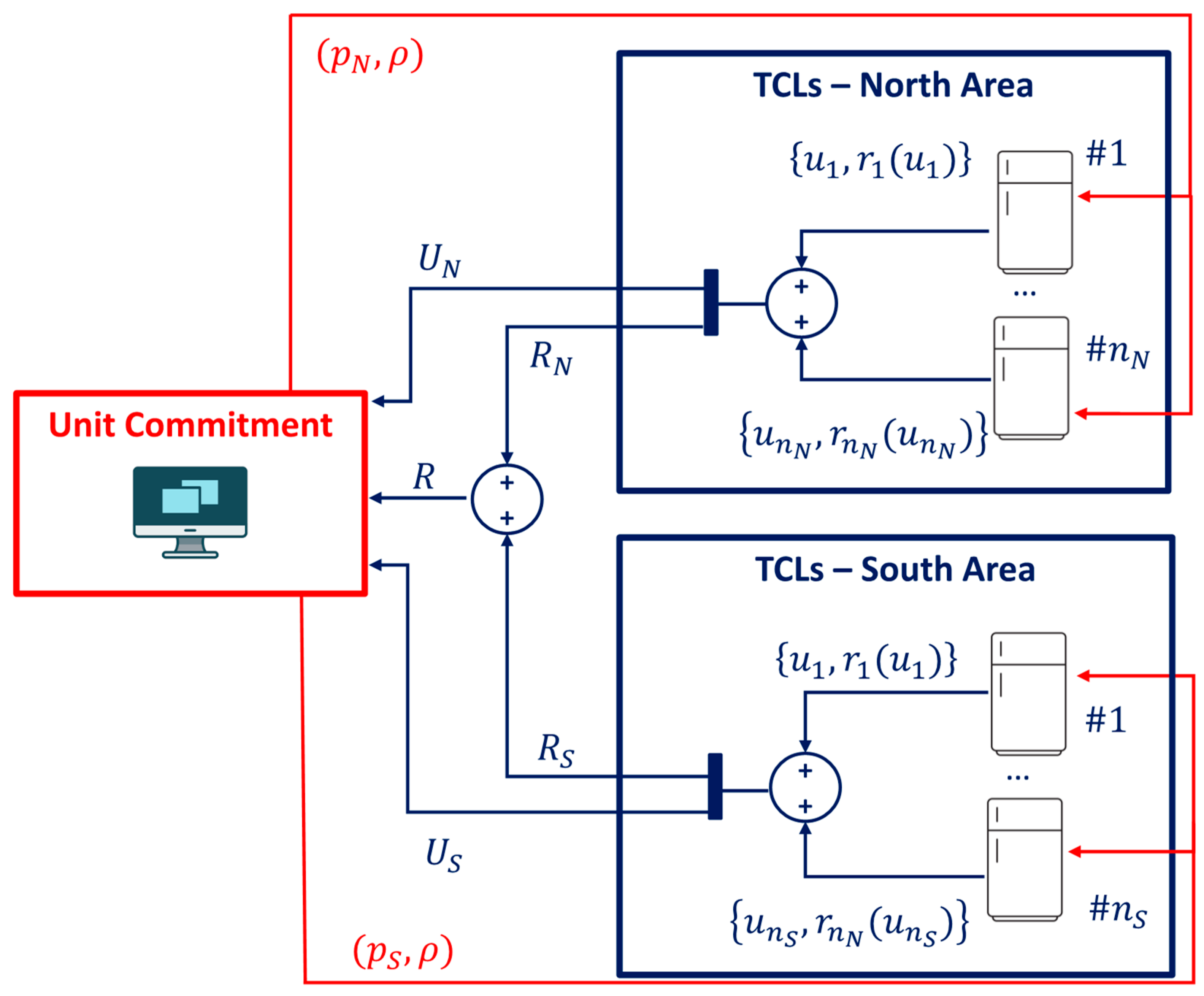
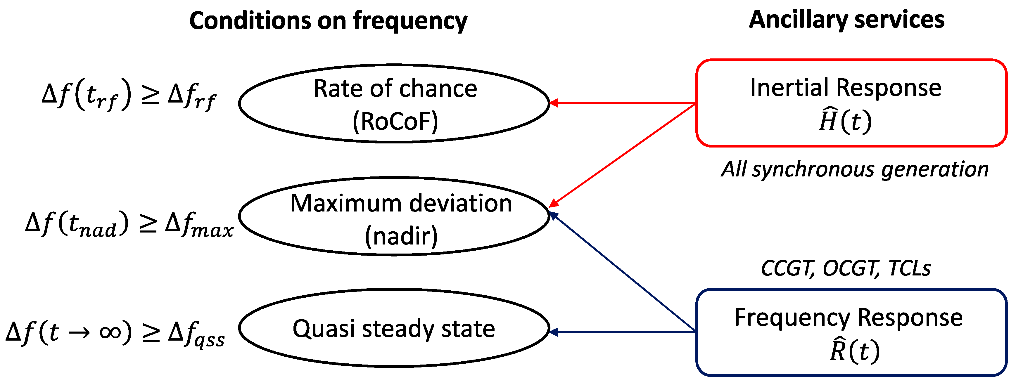
  • A novel modeling formulation based on the initial contribution in [23] is proposed and applied to the realistic case of multi-area power systems. In other words, the UC model integrates network topology constraints leading to the broadcast of multiple and area-dependent price signals to TCLs, which are distributed among the busbars of the system. Besides the novel integration of constraints on the network-topology, the UC model includes inertia-dependent frequency response (FR) constraints which participate in the characterization of the system operation, generating energy and FR price signals that account for multiple generation technologies.
  • The mean field game modeling framework proposed in [23] is extended in order to overcome the standard “players homogeneity” assumption. Ad hoc modifications of the canonical mean field game equations allow to describe a finite (low) number of diverse heterogeneous population. This is combined with clustering techniques to obtain an accurate description of a large number of heterogeneous devices. This methodological novelty is specifically utilized in this work to quantify the potential flexibility benefits of thermostatically controlled loads in a multi-area system but it could also be used in other mean field applications such as communication networks and crowd dynamics.
  • The convergence to equilibrium of the proposed modeling approach, envisaging multiple prices’ formation and multiple representative clusters of TCLs, is demonstrated through detailed case studies based on a typical 2030 Great Britain (GB) power system scenario, characterized by large penetration of renewable sources.

1.3. Paper Structure

The rest of the paper is organized as follow. Section 2 introduces the two-area power system model and presents the general framework of the interactions between TCL populations and power system scheduling. In particular, the mathematical formulation of the UC problem and the modeling of the TCL thermal dynamics are included in this section. Furthermore, Section 3 deals with the mean-field game formulation integrating the proposed TCL clustering procedure. The presentation of the case studies and the analysis of the simulative results are in Section 4. Conclusive remarks are highlighted in Section 5.

2. Model Setup and Assumptions

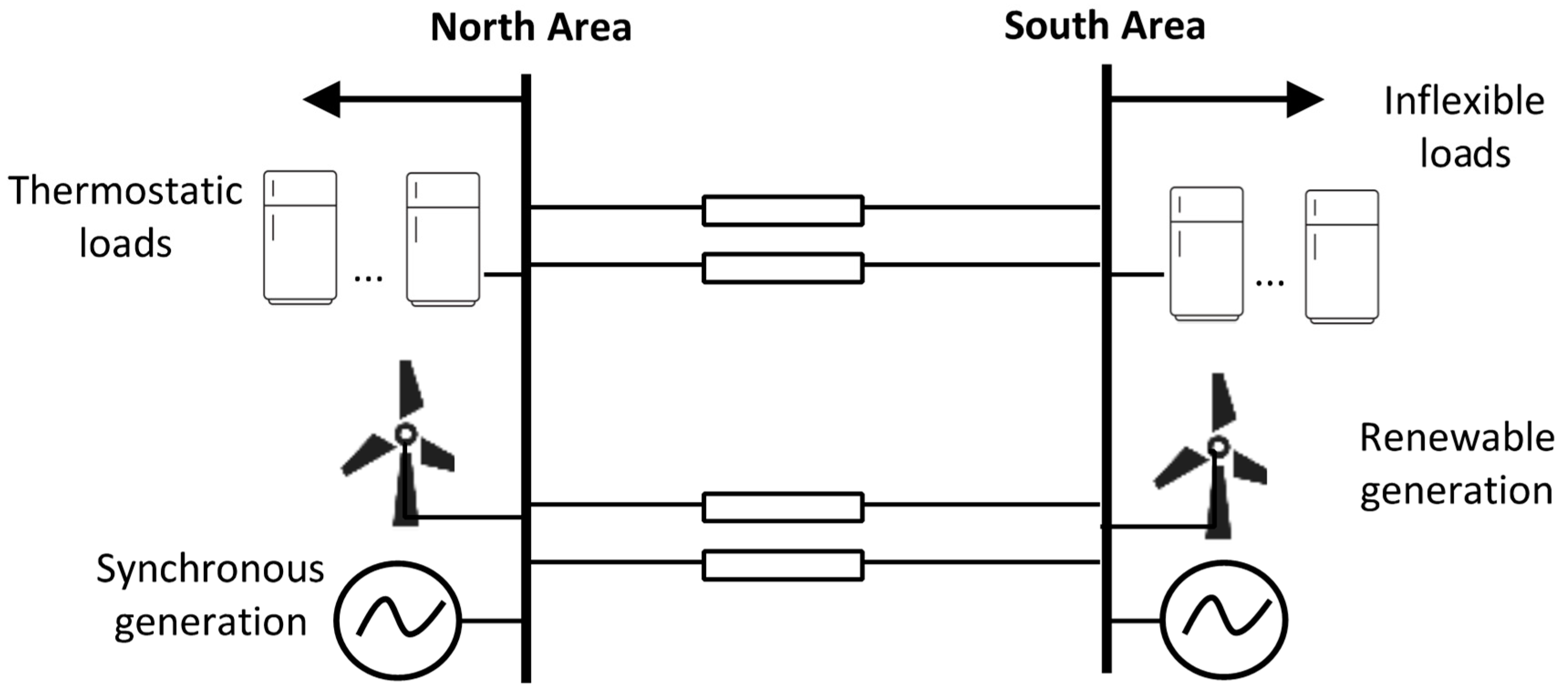
2.1. Power System Model and TCLs-System Interactions

The methodology developed in this paper can be applied to multi-area power systems with any grid topology. For simplicity reasons and without loss of generality, this work analyzes the two-area power system model illustrated in Figure 1. This can correspond, for example, to a fairly accurate representation of the whole GB system in the context of frequency control studies. Previous studies [24] simulating the frequency dynamics of a detailed GB 36-busbar model indicated the possibility to cluster the frequency dynamics at each busbar into two/three macro areas. In fact, the frequency dynamics corresponding to busbars in the same area were very much similar among each other.
Moreover, the two areas represent, respectively, the southern and northern part of the GB system. The areas are connected by overhead alternating current (AC) transmission lines and the western high voltage direct current (HVDC) link [2]. Synchronous generation technologies, such as open cycle gas turbine (OGCT), combined cycle gas turbine (CCGT) and nuclear, renewable energy sources (modeled as wind generation in this work), TCLs and inflexible loads are distributed between the two bus-bars. The power typically flows from the North Area (NA) towards the South Area (SA) due to the combination of relatively lower demand and the vaster presence of wind generation in the NA. For simplicity, HVDC links with Continental Europe and Ireland are neglected, also because these do not currently provide FR support.
This work also assumes that the frequency dynamics following a sudden and large generation outage are the same at each busbar. Hence, the FR delivered by a generator or a TCL in one area provides the same effect to the frequency dynamics of both areas. The outcomes in [24] show how (minor) differences in the frequency dynamics at each busbar would be actually registered only during the very short-term transient period (e.g., in the interval [ 0 + , 0.5 ] s). Differences are no longer reported when frequencies reach a nadir (the nadir condition coincides with the post-fault frequency deviation reaching its maximum value [2]) condition thus at quasi-steady state [24].
Under the assumptions listed above, the modeling framework proposed in this work is graphically described in Figure 2. The optimal operation and security of the power system in Figure 1 is determined through the solution of a typical UC problem. As outcome, the UC computes three price signals p N , p S , and ρ , that are broadcast to the TCLs depending on their geographical location as in Figure 2. In particular, p N and p S represent the prices of energy in the NA and SA, respectively, as suggested by the relevant subscripts N and S . These might be different in time periods where the power capacity of the NA-SA interconnector is fully employed. On the other hand, p N = p S holds if the transmission lines connecting the two areas are only partly loaded. Moreover, since the post-fault frequency dynamics were assumed to be the same at each area, the same price signal ρ , which represents the availability fee awarded for FR provision, is broadcasted to all the TCLs.
Based on the prices signals described above, each TCL computes individually its optimal operation policy that consists of two quantities, i.e., the power profile consumption u and the allocated FR r that the load is able to provide. The frequency support r of the TCL corresponds to a power reduction in case of a frequency event and therefore it is limited by the power consumption u , since it possible to provide FR only when the TCL is ON and absorbing power.
Afterwards, the operation policies of the TCL are aggregated at bus-bar level yielding the aggregate power consumptions U N and U S , and the corresponding FR allocations, R N and R S . It is worth noting that the UC treats U N and U S separately, due to the presence of constraints on power flows (i.e., Kirchhoff’s circuit laws), whereas it only necessitates of R = R N + R S , i.e., the system-level aggregation of FR provided by the TCLs (further explanations are provided in Section 2.2.2). Finally, these three quantitates modify the UC solution and therefore vary the numerical value of p N ,   p S , and ρ . A market equilibrium is reached through the iterated broadcast of updated price signals, ensuring that, at the final solution, the aggregate TCL quantities ( U N , U S , R ) obtained for a certain broadcast of ( p N ,   p S ,   ρ ), induce those very same prices when considered in the resolution of the UC problem.
The proposed coordination scheme envisages a static optimization and operation framework over a fixed time window (e.g., 24 h). For simplicity, the iterated unit commitments, price broadcasts and optimizations of the TCLs ON/OFF profiles are all determined in advance of the considered time interval, assuming perfect knowledge of all the relevant system quantities. More complex setups can be considered in a realistic framework, including for example a receding horizon paradigm that entails periodic updates of the operational strategies on the basis of updated measurements and estimations, in order to implicitly account for uncertainties and modeling mismatches.

2.2. The Unit Commitment Problem

2.2.1. Modeling Assumptions

The objective of the UC is to determine optimal decisions concerning the system scheduling (i.e., generation commitment and dispatch levels, system-wide FR allocation and power flows through the interconnectors) in order to minimize the short-term operating costs. It is worth noting that the result of the UC can be interpreted as the solution of a market clearing process, maximizing the social welfare, under typical assumptions of inelastic demand and perfect competition [25].
To simplify the analysis, the UC is formulated in a deterministic framework. In line with other works (e.g., [23,26]), the UC is presented by means of a quadratic programming formulation (quadratic objective function with linear constraints), which envisages only continuous decision variables. In particular, it is possible to assume that the size of a single plant of any generation technology g , in any area k { N , S } , is significantly smaller than P g , k m a x , i.e., the total installed capacity of technology g in area k . It follows that typical ON/OFF commitment decisions can be extended to the fleet and expressed by continuous variables H g , k ( t ) [0,1].
Moreover, the use of a quadratic programming formulation guarantees the continuity of the partial derivative of the UC solution with respect to optimization constraints’ parameters and maintains the useful economic interpretation of the Lagrange multiplier associated to the constraints as shadow prices. Under this framework and following the scheme in Figure 2, ( p N ,   p S ) and ρ will correspond to the Lagrange multipliers associated to the supply–demand balance in the two areas and to the frequency security constraints, respectively. In other words, ( p N ,   p S ) are equal to the cost of providing an additional unit of energy to the two areas, whereas ρ denotes the benefit for the system of receiving one additional unit of FR from the TCLs.
Intertemporal constraints (e.g., generation ramping) are neglected, making it possible to solve the UC problem on an instant-by-instant basis. This assumption facilitates the consistency with the time-continuous formulation of mean field game introduced in Section 3, allowing to solve the UC problem over the continuous time interval [ 0 , t f i n ] . It is worth pointing out that these simplifications are introduced for compactness of the analysis. However, they are not required under the proposed framework and more complex models of UC can in principle be used.

2.2.2. Mathematical Formulation

Let us now formally characterize the UC problem at the generic time t . First, the set ξ k ( t )   of the generation decision variables in area k = { N , S } is defined in (1) and it includes the commitment decisions H g , k ( t ) , dispatch output P g , k ( t ) , and the corresponding FR allocation Π g , k ( t ) for each generation technology g . Without loss of generality, it is assumed that the same G distinct technologies are present in both areas.
ξ k ( t ) =   { H 1 , k ( t ) H g , k ( t ) H G , k ( t ) }   { P 1 , k ( t ) P g , k ( t ) P G , k ( t ) }   { Π 1 , k ( t ) Π g , k ( t ) Π G , k ( t ) } .
In the current analysis, the allocated FR corresponds to the aggregate power headroom of each generation technology that can be provided in response to frequency events. Moreover, in accordance with the schematics in Figure 2, the total TCL power consumption at a generic area k is U k ( t ) , whereas the system-level allocated FR from TCLs is R ( t ) . Having characterized these quantities, the UC at time t can be described through the following optimization problem:
φ ( U N ( t ) , U S ( t ) , R ( t ) ) =   min ξ N ( t ) , ξ S ( t ) , F ( t ) k { N , S } g = 1 G a k , g · H g , k ( t ) P g , k m a x + ε k , g · P g , k ( t ) + η k , g · P g , k 2 ( t ) .
In the proposed formulation, the UC objective function is equal to the sum (over all areas k and technologies g ) of the no load cost a k , g · H g , k ( t ) P g , k m a x   and of the quadratic generation costs, parametrized by ε k , g and η k , g . It should be emphasized that there is no explicit formulation of a cost function for FR provision by generation. This is implicitly accounted for as the opportunity cost of not providing energy and increasing the on-line capacity to maintain headroom for FR. Note also that the aggregate power consumptions U k ( t ) and allocated FR R ( t ) of the TCLs appear as parameters of the optimal solution φ , as they are considered fixed quantities in the optimization and are determined independently by the TCLs in response to broadcast prices.
The objective function (2) is subject to the following constraints:
0 H g , k ( t ) 1                   g { 1 G }                   k { N , S }
Π g , k ( t ) δ g , k · H g , k · ( t ) P g , k m a x                   g { 1 G }                   k { N , S }
Π g , k ( t ) s g , k · [ H g , k ( t ) · P g , k m a x P g , k ( t ) ]                   g { 1 G }                   k { N , S }
μ · χ g , k · H g , k ( t ) . P g , k m a x P g , k ( t )                   g { 1 G }                   k { N , S }
g = 1 G P g , N ( t ) F ( t ) U N ( t ) L N ( t ) = 0
g = 1 G P g , S ( t ) + F ( t ) U S ( t ) L S ( t ) = 0
F m a x F ( t ) F m a x
2 θ · t r f · t d t r f 2 R ^ ( t ) 4 f r f · t r f · H ^ ( t ) 0
q ^ ( t ) R ^ ( t ) · H ^ ( t ) 0
θ D [ L S ( t ) + L N ( t ) + U S ( t ) + U N ( t ) R ( t ) ] · f q s s R ^ ( t ) 0 .
The inequalities (3) follow from the definition of H g , k ( t ) as percentage of the online generation capacity. Constraints (4) and (5) ensure the feasibility of the allocated FR from generators. This is bounded by the headroom χ g , k · H g , k · ( t ) P g , k m a x in (4) and by the slope s g , k , linking it with the dispatch level P g , k ( t ) in (5). Constraint (6) prevents trivial solutions with large values of the commitment variables H g , k (proportional to the inertial response of the generation technology) with large Π g , k and zero P g , k . In fact, the dispatch output has to be μ -times larger than the allocated FR headroom. The equalities (7) impose the generation/demand balance in each area. In this case, the power flow F ( t ) through the transmission lines connecting the two areas is assumed to be positive when the power flows from N to S. The total demand in each area k is given by the sum of the local TCL consumption U k ( t ) and the consumption of the inflexible load L k ( t ) . The feasibility of the power flow through the interconnectors is ensured by (8). For simplicity, one large interconnector is modeled rather than single links individually.
In the aftermath of a sudden generation loss θ , the system level requirements for FR and inertial response that guarantee secure frequency dynamics are obtained by (9)–(11). For compactness, the post-fault inertial response H ^ ( t ) and the system-level FR R ^ ( t ) are defined in (12):
H ^ ( t ) = k { N , S } g = 1 G h g , k H g , k ( t ) · P g , k m a x h θ θ f 0
R ^ ( t ) = k { N , S } ( g = 1 G Π g , k ( t ) ) + R k ( t ) .
Note the H ^ ( t ) includes the constant of inertia h θ of the maximum infeed loss θ since the latter no longer supports the system. It is assumed that OCGT and CCGT technologies provide both inertia (i.e., they have a positive factor   h g , k )   and FR (with Π g , k greater than zero). In accordance with the typical system operation in GB, nuclear generation only contributes to the inertial response, since it is operated fully loaded, with no headroom for FR. Wind generation does not provide any ancillary service, consistently with current and typical configurations [27]. Finally, TCLs can only contribute to the provision of FR through the aggregated term R k ( t ) in (12b).
The complete mathematical derivation of the constraints (3)–(11) was presented in [28,29]. These constraints implement the interactions illustrated in Figure 3 between the ancillary services and the conditions to be maintained to ensure the security of the system.
Constraint (9) depends only on H ^ ( t ) and guarantees that the negative frequency deviation, evaluated in the relevant time window t r f of the rate of change of frequency (RoCoF), remains above a specified threshold f r f . The ability to contain the frequency deviation at the nadir above the maximum negative deviation f m a x is ensured by (10), which recognizes the interaction of H ^ ( t ) and R ^ ( t ) as in Figure 3. The results in [28,29] have demonstrated that, for a given system condition at time t , there exists a unique q ^ ( t ) = R ^ ( t ) · H ^ ( t ) such that f ( t n a d ) = f m a x . Moreover, since the left-hand side of (10) is convex in the considered range of values for R ^ ( t ) and H ^ ( t ) , the constraint is linearized around a number n l = 10 points x l = { H ^ l , R ^ l }   l   { 1 n l } such that z ( H ^ l , R ^ l ) = q ^ . Finally, in accordance with Figure 3, (11) allocates enough R ^ ( t ) such that the quasi-steady-state frequency deviation is above f q s s .

2.2.3. Characterizing the Energy and FR Prices

In the previous subsection, the optimal solution of the UC problem has been defined in (2) as a function φ of ( U N ( t ) , U S ( t ) , R ( t ) ) , i.e., the total power consumptions of the thermostatic loads in the two areas and their allocated FR. In accordance with the paradigm illustrated in Figure 2, these quantities are not decision variables of the UC problem, since they derive from the operation profiles of the thermostatic loads, which are determined independently by each TCL. Under this framework, let us define the following quantities
p N ( t ) = φ ( U N , U S , R ) U N | U N = U N ( t ) U S = U S ( t ) R = R ( t )
p S ( t ) = φ ( U N , U S , R ) U S | U N = U N ( t ) U S = U S ( t ) R = R ( t )
ρ ( t ) = φ ( U N , U S , R ) R | U N = U N ( t ) U S = U S ( t ) R = R ( t )
The quantity p N ( t ) corresponds to the cost of accommodating one additional unit of TCL power consumption in the NA. From (7a), this is equivalent to the marginal cost of energy and therefore p N ( t ) can be considered as the electricity price paid by the TCLs in the NA at time t . The extension of this reasoning characterizes p S ( t ) as the price paid by the TCLs in the SA at time t . With a similar rationale, ρ ( t ) represents the marginal saving in the optimized system costs φ when one additional FR unit is being provided by the TCLs. It follows that ρ ( t ) can be interpreted as the availability price paid to the TCLs for the allocation of FR. Pursuant to the assumptions in Section 2.1, ρ ( t ) is independent of the geographical location of the TCLs.
Note that p N ( t ) and p S ( t ) in (13a) and (13b) correspond to the Lagrange multipliers of the constraints (7a) and (7b), respectively. Similarly, the price ρ ( t ) in (13c) depends on the FR constraints (9)–(11). In the simulations presented in this paper, it results that (10) is the only active constraint among (9)–(11) for any time period t , and therefore ρ ( t ) is equal to the Lagrange multiplier associated to (10). In general, ρ ( t ) can always be calculated with a variational approach, i.e., as the ratio Δ φ R where Δ R is a sufficiently small FR variation and Δ φ is the resulting change in the minimized UC costs.

2.3. Modeling Thermostatically Controlled Loads

Having provided an analytical description of the UC problem and of the price signals (red elements in Figure 2), this subsection focuses on the characterization of the TCLs in terms of temperature dynamics and operational decisions in response to price signals (blue elements in Figure 2). Since the internal temperature T of a single TCL does not depend on the geographical location of the appliance, the area index k = { N , S } is dropped in the notation of this section. Hence, the temperature profile T ( t ) of a single TCL is the solution of the first order differential equation
T ˙ ( t ) = ( T ( t ) ,   u ( t ) ) = 1 σ ( T ( t ) T o f f + ζ · u ( t ) )
T ( 0 ) = T ˜ .
where T ˜ denotes the initial temperature at time 0 and u ( t ) { 0 , Γ } represents the power consumption of the TCL at time t . Consistently with the typical characteristics of thermostatic loads, u can either be equal to 0 (OFF state) or to the nominal power Γ (ON state). The thermal time constant of the device is denoted by σ , while T o f f and ζ represent the ambient temperature and the heat exchange model, respectively. Following the formulation proposed in [23], a second state variable I ( t ) = T ( t ) T ˜ is introduced to indicate the variation of the internal TCL temperature in the time interval [ 0 , t ] . From (14), the dynamic equation of the second state variable is I is straightforward to derive as:
I ˙ ( t ) = T ˙ ( t )
I ( 0 ) = 0
.
The variable I ( t ) was included in the dynamic model for antisynchronization purposes, as it allows to differentiate the behavior of the single devices within the TCL population. In particular, the state variable I ( t ) allows to distinguish TCLs that, at a certain time t , have reached the same temperature T ( t ) from different initial values T ˜   (as their net temperature variation I ( t ) = T ( t ) T ˜ will be different). This enables a TCL coordination strategy that, by introducing a setpoint for I , is able to diversify the behavior of the loads, facilitating the convergence of the proposed control scheme to an equilibrium solution. Having characterized the temperature dynamics of the TCL in terms of its ON-OFF power consumption u ( t ) = { 0 , Γ } , it is now possible to quantify its FR contribution as a function r of its internal temperature T and power consumption u :
r ( T ( t ) ,   u ( t ) ) = λ ( T ( t ) ) · u ( t ) .
Recall that the TCL is able to provide FR by reducing its power consumption in case of a frequency event and therefore   r 0 only in the ON state, when u ( t ) = Γ . The additional factor λ ( T ( t ) ) is used to limit the FR provision and avoid violations of the temperature constraints. As in [23], λ : [ T m i n , T m a x ] [ 0 , 1 ] is a decreasing function of the internal temperature T such that λ ( T m a x ) = 0 and λ ( T m a x ) = 1. Here, T m a x and T m i n are the operational upper/lower temperature thresholds of the TCL. Moreover, it is assumed that λ evolves linearly with T
λ ( T ) = ( T T m a x ) / ( T m i n T m a x ) .
When T =   T m a x   a n d   λ ( T ) = 0 , the TCL must remain in its ON state in order to not exceed its maximum temperature state and therefore cannot provide any FR. Conversely, when T =   T m i n   a n d   λ ( T ) = 1 , the load can switch-off without violating the temperature constraints and the full amount of FR can be provided.

The Agent-Based Approach

Each TCL is modeled as a selfish rational agent that, on the basis of the broadcast energy and FR prices made explicit in (13), independently determines its power profile u (and associated FR allocation r ) in order to optimize its objective function. For the TCLs in each area k { N , S } , this corresponds to the minimization of the functional J k :
J k ( u k ( × ) ) = 0 t f i n p k ( t ) u k ( t ) ρ ( t ) r k ( T ( t ) ,   u k ( t ) ) + α ( T ( t ) T ¯ ) 2 + β ( I ( t ) I ¯ ) 2 d t + Ψ ( I ( t f i n ) )
subject to:
T ( 0 ) = T ˜
I ( 0 ) = 0
T ( t ) [ T m i n , T m a x ]                     t [ 0 , t f i n ]
Each of the terms in (18) are briefly described in Table 1.

3. The Mean Field Game Formulation

In the chosen framework, the TCLs are modeled as independent agents that determine their ON/OFF operational profile in response to broadcast price signals, scheduling power consumption at low energy prices p and FR provision at high availability fees ρ . The competing interactions between the loads correspond to the impact of their operational strategies on price formation (the more power is consumed at a certain time period, the higher the electricity price will be). The objective of this section is to characterize an equilibrium solution where any single TCL has no interest in unilaterally modifying its power consumption profile, given the energy and FR prices set in (13).
Given the typically low power consumptions of real TCLs (e.g., domestic refrigerator) with respect to the total system demand, it is possible to infer that the single device does not significantly impact the system prices. However, the behavior of the aggregate TCL population has a non-negligible impact on price formation that needs to be considered. In order to derive a compact model of this effect in scenarios with large populations of thermostatic loads (in the order of millions), the TCL coordination problem is described as a mean field game, i.e., a game with an infinite number of players where the objective function of the single agent is only affected by the aggregate behavior of the players’ population.
Following the approach in [23], two coupled partial differential equations (PDEs) are used to describe the optimal behavior and the dynamics of the TCLs in each area k { N , S } .
  • The first PDE is an Hamilton–Jacobi–Bellman equation that returns the value function V associated to the TCL optimization problem. Denoting the argument of the integral (18) with A k ( u , T , I ) , this can be defined as:
    V t ( k ) ( t , T , I ) = min u { 0 , Γ } [ A k ( u k , T , I ) + ( V T ( k ) ( t , T , I ) + V I ( k ) ( t , T , I ) ) · k ( T , u k ) ]
    where V x denotes the partial derivative of V with respect to x . According to the dynamic programming principle [30], this equation can be integrated backward in time to determine the optimal control of the individual TCL as a function of time t and its temperature variables T and I , according to the following expression:
    u k * ( t , T , I ) = a r g   m i n u { 0 , Γ } [ A k ( u k , T , I ) + ( V T ( k ) ( t , T , I ) + V I ( k ) ( t , T , I ) ) · k ( T ,   u k ) ] .
  • The second PDE is a transport equation which characterizes the evolution in time of the state distribution m ( k ) when u k * is applied:
    m t ( k ) ( t , T , I ) = [ m t ( k ) ( t , T , I ) · ( t , u k * ( t , T , I ) ) ] T [ m t ( k ) ( t , T , I ) · ( T , u k * ( t , T , I ) ) ] I
    m k ( 0 , T , I ) = m 0 ( T ) · δ ( I ) .
This equation is integrated forward in time to determine m ( k ) ( t , T , I ) , i.e., the fraction of TCLs in area k   whose temperature variables are equal to T and I at time t . Note that the boundary condition (22b) is consistent with (19b), as the Dirac delta function indicates that all loads have I ( 0 ) = 0 and their initial temperature T ˜ follows the distribution m 0 ( T ) .
Denoted by n N and n S the total number of TCLs located in the NA and the SA, respectively, it is possible to provide a closed-form expression of the aggregated power consumptions U N ,   U S , and allocated FR R when the optimal control u * is applied. These quantities, denoted with a star subscript, are equal to the following weighted integrals:
U N ( t ) = U N * ( t ) = n N · I m i n I m a x T m i n T m a x u N * ( t , T , I ) · m N ( t , T , I ) d T d I
U S ( t ) = U S * ( t ) = n S · I m i n I m a x T m i n T m a x u S * ( t , T , I ) · m S ( t , T , I ) d T d I
R ( t ) = R * ( t ) = I m i n I m a x T m i n T m a x [ n N · r N ( T , u N * ( t , T , I ) ) m N ( t , T , I ) ] + [ n S · r S ( T , u S * ( t , T , I ) ) m S ( t , T , I ) ] d T d I .
It is worth highlighting the interactions between the mean field game equations. The temperature distributions m ( k ) in (22) depend on the power consumption profiles u k * and the value functions V ( k ) in (20). On the other hand, the distribution m ( k ) in (22) has a direct impact on U N ,   U S , and R through (23). The dependencies of these aggregate power/response quantities on the temperature distributions m ( k ) , albeit relevant, are not indicated explicitly in (23) and in the associated equations for simplicity of notation. Note in fact that the quantities U N ,   U S , and R affect the price signals p N ,   p S , and ρ in (20) through the UC solution of (2) and the price dynamics (13). In order to account for these complex interdependencies, the proposed solution of the distributed coordination problem for large populations of TCLs corresponds to the quantities ( p k ,   ρ , V ( k ) , u k * , m ( k ) , U k ,   R ) ,   k { N , S } that satisfy (13), (20)–(23). From the framework illustrated in Figure 2, at the proposed solution the TCLs autonomously apply their best operation policy u N * or u S * in response to the price signals p N ,   p S , and ρ and, by doing so, their corresponding aggregate quantities U N ,   U S , and R induce those very same price signals in the unit commitment problem (2)–(11).

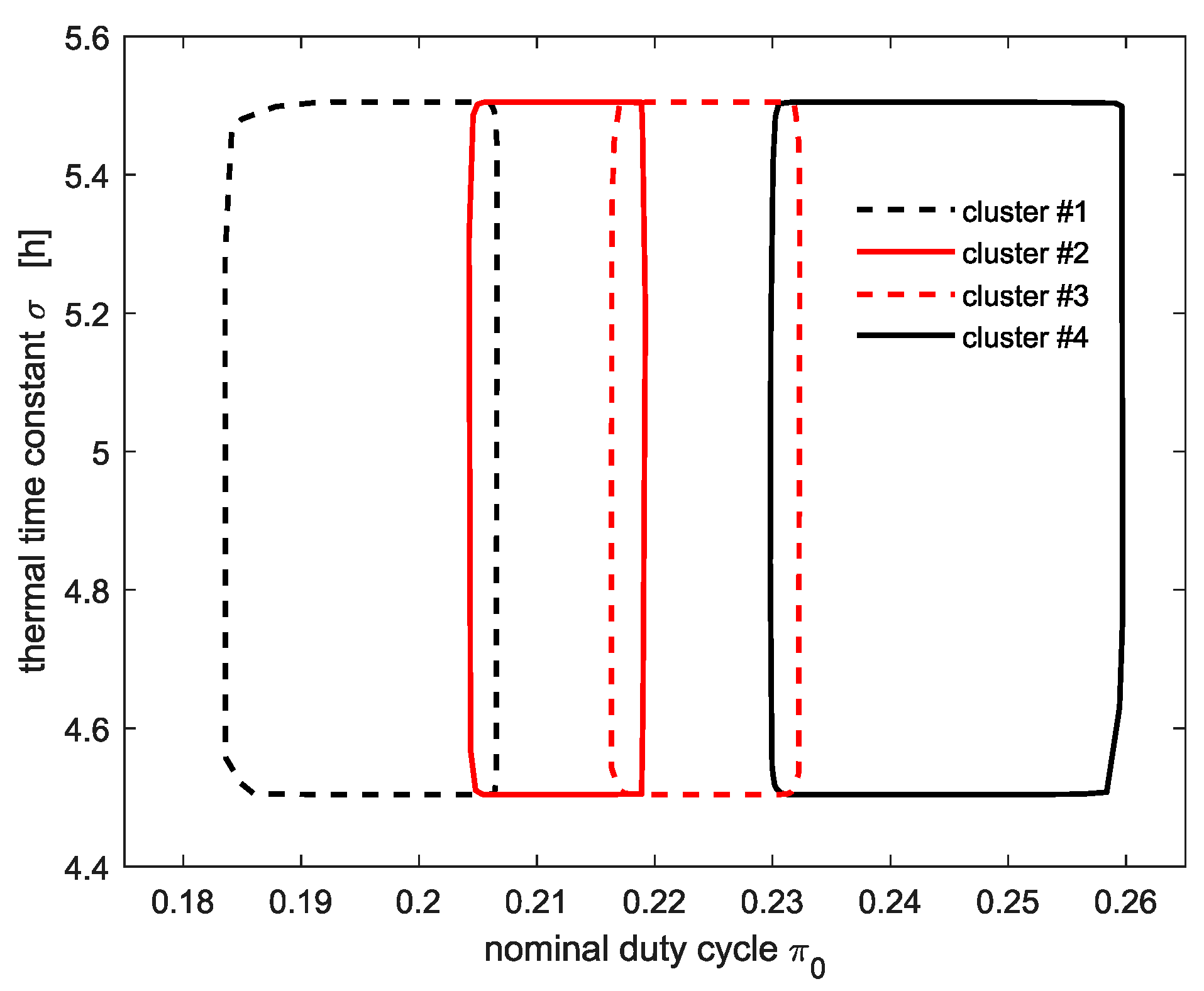
3.1. Clustering the Population of TCLs

One fundamental assumption in standard MFG formulations is homogeneity of the agents: the mean field game equations are able to compactly describe the interactions between the different agents only if these have the same dynamics and equal parameters. The proposed MFG equations (20)–(23) follow this typical paradigm and consider TCLs that are indistinguishable. However, in practical applications, large groups of TCLs are rarely perfectly homogeneous. This subsection aims at extending the previous formulations to populations of heterogenous TCLs, introducing clusters of thermostatic loads with similar parameters and modifying ad hoc the MFG equations.
Considering the realistic restrictions imposed by heterogeneous parameters, the authors in [6] defined a lowest-common-denominator model for the appliance capabilities, without being unnecessarily conservative. This way, despite their intrinsic differences, all TCLs could be characterized by the same representative envelope parameters. Note that this envelope model established a lowest-common denominator for the flexibility of all appliances, but it did not necessarily represent any specific device in the population.
The methodology developed in [6] is applied in this work to acknowledge the actual heterogeneous nature of a population of TCLs and, at the same time, to maintain a simple and common description of all the TCLs. In fact, regardless of the geographical location, a set of representative parameters is used to describe all n N + n S TCLs. This assumption is acceptable as long as the devices do not vary significantly. In case of largely heterogeneous appliances, it may be beneficial to partition the population into clusters of TCLs with more similar capabilities. It will be possible to assign different representative parameters to the TCLs in each cluster as presented in [6].
To do so, the initial population of n N + n S devices has to be divided into a number C of clusters c with c { 1 , , C } . The partitioning is performed using the k-means clustering algorithm (based on [31]), where devices are clustered based on their distance in parameters’ space. Considering a set of data X = { x 1   x n N + n S } , where each of the data is a γ -dimensional vector of attributes i.e., the user-defined TCLs’ parameters σ , T m i n , T m a x , etc., the k-means clustering algorithm aims to partition the n N + n S data into a number C of sets Ω (with Ω = { Ω 1 Ω C } and C n N + n S ) by finding
arg   min Ω c = 1 C x Ω c x δ c 2 .
Note that δ c represents the mean of all the data included in Ω c .
It is worth highlighting that the aim is simply to divide TCLs into sets of similar appliances and not to identify strictly separated clusters in parameters’ space. Hence, there is no unique optimal cluster count: a reasonable number of clusters could be determined from its impact on subsequent optimization steps. Finally, the authors point out that the k-means algorithm is a stochastic algorithm, so that cluster assignments are likely to differ between repeated cluster attempts.
The relevant simulations performed in this work in order to cluster the overall TCLs’ population were employed the Matlab built-in function kmeans [32].
An illustrative example of the clustering process is offered in Figure 4. A population of 20 , 000 heterogeneous devices is created by varying by ±10% the typical parameters σ , T m i n , T m a x , T o f f , T o n , of domestic fridge-freezers [6], where T o n = T o f f ζ · Γ is the asymptotic cooling temperature. Note that, rather than directly considering T m a x and T m i n , the ±10% parametric variation is applied to 0.5 · ( T m a x + T m i n ) and ( T m a x T m i n ) , to simulate variability in the set-point temperature and deadband width, respectively. The entire population of TCLs is inscribed within the external perimeter of the graph in Figure 4, where the y-axis shows the thermal time constant σ and the x-axis refers to the nominal duty cycle π 0 of the device, expressed as follows:
π 0 = l o g ( T m a x T o n T m i n T o n ) / l o g [ ( T m a x T o n ) ( T m i n T o f f ) ( T m i n T o n ) ( T m a x T o f f ) ] .
In the example in Figure 4, the TCL population is partitioned into four clusters of TCLs with similar characteristics. The clusters have different sizes since 42,272 TCLs are in the first cluster (dashed black line), 34,901 in the second (red solid line), 61,558 in the third (dashed red line), and 60,269 in the fourth and last one (black solid line).
Low values of σ may indicate TCLs with poor insulation. Similarly, clusters with large values of π 0 include TCLs that would on average absorb more energy.
The fundamental methodology presented in the previous sections does not change notably as the UC problem only deals with aggregate TCL values and the very same prices (13) are broadcast to all TCLs regardless their reference cluster (in accordance with Figure 2). However, since a different set of representative parameters is assigned to each cluster of TCLs, the mathematical formulation of the mean field game Equations (23a)–(23c) requires some modifications. In particular, a distinct set of Equations (20)–(22) will be considered not only for each area k but also for each distinct TCL cluster c , obtaining in each case a different power consumption profile u N , c * ( t , T , I ) and allocated FR r k , c ( T , u k , c * ( t , T , I ) ) . Their aggregated values over the whole TCL population can then be expressed as:
U N ( t ) = U N * ( t ) = I m i n I m a x T m i n T m a x c = 1 C n N , c · u N , c * ( t , T , I ) · m ( N , c ) ( t , T , I ) d T d I
U S ( t ) = U S * ( t ) = I m i n I m a x T m i n T m a x c = 1 C n S , c · u S , c * ( t , T , I ) · m ( N , c ) ( t , T , I ) d T d I
R ( t ) = R * ( t ) = I m i n I m a x T m i n T m a x k { N , S } c = 1 C [ n k , c · r k , c ( T , u k , c * ( t , T , I ) ) · m ( k , c ) ( t , T , I ) ] d T d I .

3.2. Enabling the Smart Control of TCLs

This section deals with practical considerations on two possible implementation schemes for smart TCLs under the proposed coordination mechanism. Both schemes are suitable for multi-clustered populations of TCLs. The first envisages requires a bidirectional communication infrastructure between single TCLs and the so-called central coordinator (e.g., the TSO or an aggregator). Based on some estimate of the total power consumption and allocated FR of the TCLs, the coordinator (i) solves the UC problem, (ii) determines the associated prices for energy (at each area) and FR, and (iii) broadcasts them to individual TCLs. The appliances, in turn, determine their optimal strategy and communicate it to the coordinator, which aggregate all the information on energy and FR received. These quantities are compared with their corresponding initial values to assess whether a new solution of the UC has to be performed or convergence to the equilibrium solution has been obtained.
The second approach necessitates a one-direction communication channel only. In fact, the coordinator knows in advance the dynamics and the initial temperature distribution (22b) of the TCLs. This information might be the result of an estimation from the coordinator or may have been simply communicated to this entity by the TCL (or the TCL’s manufacturer) when joining in any flexibility contract (this approach is in line with conventional generators exchanging with the system operator their own fundamental parameters and characteristics concerning fast frequency control). Within this framework, the central coordinator can internally emulate the iterative coordination algorithm presented in this work and autonomously calculate the equilibrium solution. The price quantities associated to this equilibrium solution can be eventually broadcasted to TCLs. The devices would calculate their optimal solution in response to these prices, de facto inducing the desired equilibrium solution in one step.
Furthermore, three fundamental technical components are necessary to enable the proposed price-based control framework for distributed TCLs. The first is the TCL controller which performs calculations based on available signals and commands the actuator for relevant switching. This component can be embedded in the TCL when manufactured or installed afterwards. The second component is the smart meter to communicate to the central entity the relevant power/FR profiles scheduled by the single TCL and record the actual behavior of the TCL operating in accordance with the optimal profiles. Moreover, it will calculate, store, and communicate the corresponding costs and revenues that are associated to the operation of the TCLs, on the basis of the received price signals. It is worth noting that the smart meters’ rollout is independent of the actual deployment of TCL controllers. In other words, smart meters are already being installed although the provision of demand side response services from TCLs is still limited.
The last component is the communication infrastructure to exchange and record signals. Three classes of signals are envisaged. The first deals with quantities directly related to TCLs e.g., the internal temperature of the appliance in the case of refrigerators. The second class refers to locally available signals not directly linked to TCLs such as ambient temperature, network frequency, time. The last class refers to external signals. In the case of the proposed control strategy, the TCL controller will need to receive energy and FR prices. The TCLs will also need to communicate to the central entity their chosen profiles of power consumption and allocated FR. Note that these signals are not required to be exchanged in real time. As a result, ad hoc communication channels are not required, and the smart-metering infrastructure can be used instead.

4. Case Studies and Results

The equilibrium solution to the TCLs coordination problem expressed by (2)–(11) and (20)–(23) may be difficult to solve analytically. For this reason, a numerical approach, based on an iterative resolution scheme, is adopted. The relevant equations are solved sequentially, employing the solution of the previous step as the starting point for the resolution of the next equation. The input quantities of each equation are determined as the convex combinations of their previous and new solutions. The associated convexification parameter can be chosen to be sufficiently small as to ensure numerical convergence in all the considered case studies. Regarding the resolution of the individual equations, each PDE in (20)–(22) is integrated using finite differences schemes. The Hamilton–Jacobi–Bellman Equation in (20) is solved with an upwind scheme that is particularly suited for the ON/OFF features as the TCLs, as it selects backward/forward derivatives depending on the sign of the control variable (i.e., the power consumption of the device). A Lax–Friedrich scheme is instead used for the transport Equations (23a)–(23c), including a viscosity term to obtain a sufficiently smooth solution. More details on the actual implementation of these methodologies are provided in [23].

4.1. Numerical Assumptions

The distributed coordination strategy (DCS) presented in this work is tested in simulation, considering a typical 2030 scenario of the GB system ([2,23,28]), described through the two-area model in Figure 1. The case studies consider G   = 4 generation technologies whose characteristics are reported in Table 2, in line with the assumptions on their ability to provide ancillary services introduced in Section 2.2.2 and the numerical values in [23,28]. In accordance with the outlook of the current and future GB system discussed in [2], the installed capacity of the conventional generation is higher in the SA, whereas the NA sees a higher wind installed capacity. This reflects large the large penetration of off-shore wind farms in the northern part of the GB.
Other relevant system-level parameters are h θ   = 6 s and θ = 1800 MW, f 0   = 50 Hz, μ   = 2, t r f   = 0.5 s, t d   = 10 s, Δ f m a x   = −0.8 Hz, Δ f r f = Δ f q s s   = −0.5 Hz, and D   = 0.5/ f 0 [28]. For the simulations performed in this work, the optimization horizon was limited to t f i n = 24h. A typical winter working-day profile of the GB demand was chosen to simulate the consumption of the inflexible loads [28], assuming a 15–85% repartition of the load between the SA and the NA, resembling the typical repartition of the GB load [2]. The wind profiles used for simulation were also taken from the database in [28] (information on the numerical values of the demand profiles are shown in Appendix B in Figure A1a,b (dashed black lines), for the SA and NA, respectively. The wind profiles are shown in Figure A1c). The capacity of the interconnectors linking the NA to the SA is F m a x = 7000 MW [2].
The class of TCLs adopted for the simulation encompass domestic fridge-freezers. In the Base Case (BC), i.e., when all the TCLs are described through a single large cluster, 20 million appliances are considered. As for the inflexible loads, 85% of TCLs are assumed to be in the SA and the remaining in the NA (corresponding to n S = 17 · 10 6   and n N = 3 · 10 6 ). In the BC, all TCLs are represented by the same set of parameters σ = 4.55 h, T m i n = 22.6 °C, T m a x = 16.08 °C, T o f f = 21.98 °C, T o n = 136.1 °C, and Γ = 180 W, resulting in a steady-state power consumptions of 798.88 MW in the SA and 140.98 MW in the NA. The initial temperature distributions m N , 0 , m S , 0 are assumed to be uniform across the temperature interval [ T m i n , T m a x ] . The numerical values of the parameters in Table 1 are α = 0.2 · 10 4   £/h(°C)2, T ¯ = 0.5 · ( T m a x + T m i n ) °C, β = 0.2 · 10 4   £/h(°C)2, and I ¯ ( t ) = 0.5 + cos ( 0.9 · t ) . The choice of a periodic function for I ¯ ( t ) aims to mimic the typical intraday variational trend in the TCLs internal temperature. Finally, Ψ ( I ( t f i n ) ) = Λ · I 2   with Λ = 10 3 £/(°C)2.

4.2. Simulation Results of the Base Case

The proposed DCS was applied to the BC, considering the two-area UC problem in Section 2 and the mean field game formulation in Section 3, where all TCLs are characterized by the same representative parameters. Starting from initial solutions U N ( t ) =   U N , 0 , U S ( t ) =   U S , 0 , and R ( t )   =   R 0 = 0 t [ 0 , t f i n ] , the iterative algorithm determining the equilibrium solution converges in 150 iteration. Simulations were performed in MATLAB environment on a standard laptop ASUS EliteBook with an Intel(R) Core (TM) i7-8750H CPU (2.20 GHz) and 16 GB of RAM. The simulation time of the DCS under the BC assumption (number of clusters C = 1) was 19 min.

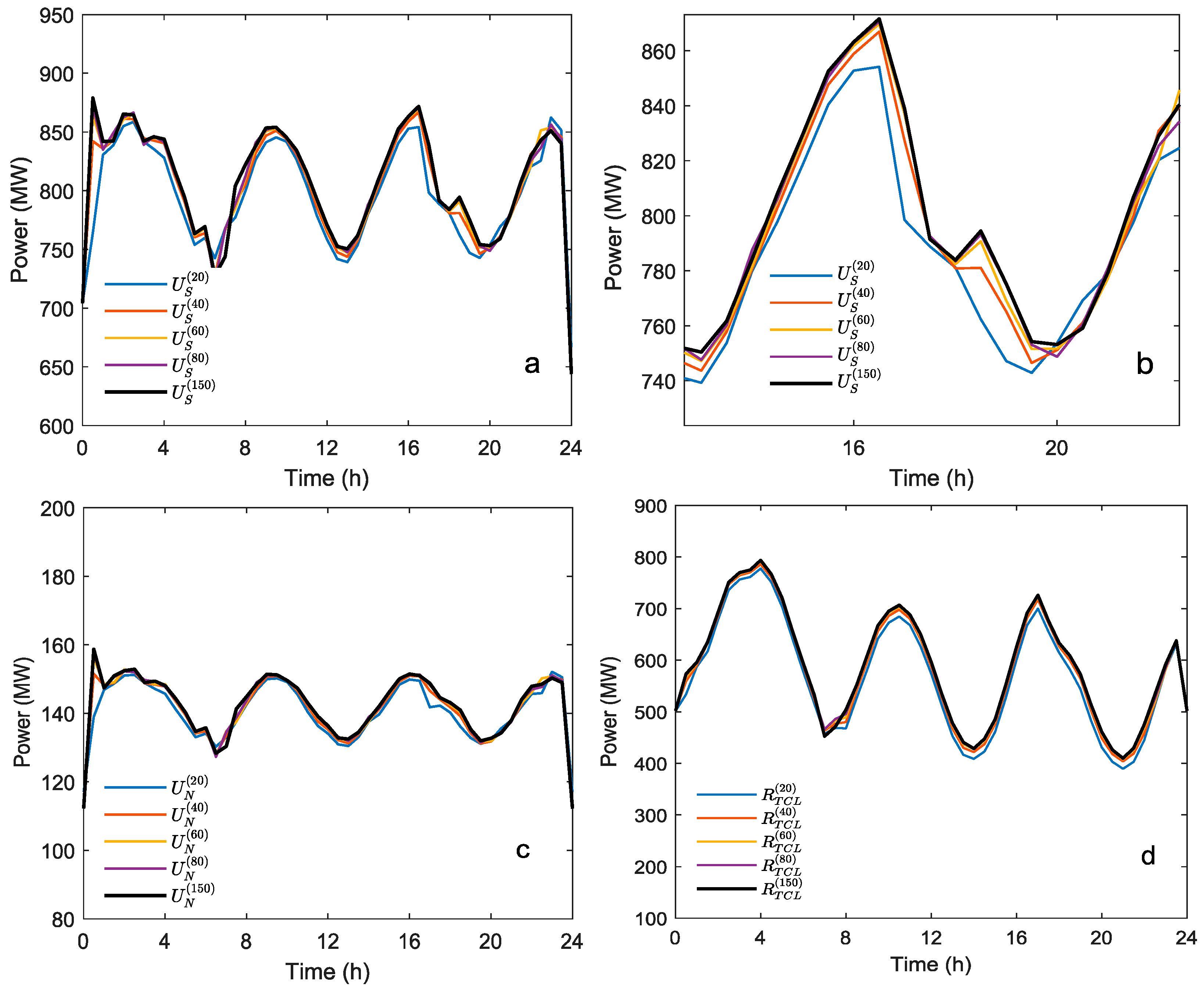
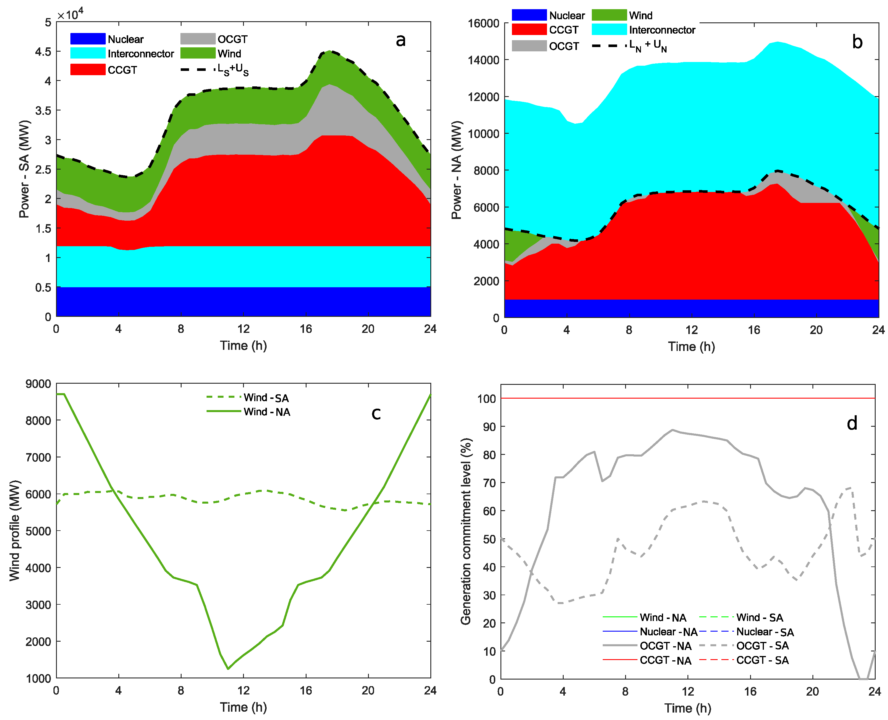
4.2.1. TCL Aggregate Consumption and Energy/FR Prices

The resulting TCL power consumptions U S ( t ) and U N ( t ) are reported in Figure 5a,c, respectively, with Figure 5b providing a zoom of U S ( t ) on a reduced time interval. The total FR allocated from TCLs, R ( t ) , is shown in Figure 5d. These three profiles are illustrated at different iterations, showing the ability of the DCS to converge to the equilibrium solution (represented in black) in a relatively low number of steps. Note that the iteration number is indicated by the superscript in brackets. This result can be better appreciated in Figure 5b. A more remarkable distance from the equilibrium solution (black line) characterizes the lines in blue and red. These refer to the solutions at the 20th and 40th iteration, respectively. The distances from the equilibrium solution are reduced in subsequent iterations until they finally overlap, having reached the equilibrium. Similar results illustrated in Figure 5b and concerning U S ( t ) are obtained for U N ( t ) in Figure 5c and for R ( t ) in Figure 5d.
Besides the convergence, the results in Figure 5 show coherent price-driven behaviors. In fact, the power consumption profiles increase during the night hours of the day, when energy prices are typically low (as confirmed by the results in Figure 6). On the other hand, low power consumptions coincide with high energy prices during the time interval 16:00–20:00. Similar trends are shown by the FR allocation, which is higher during the night hours when the system-level requirements are generally higher (low inertial response available). An opposite situation can be registered during the late afternoon/evening hours. It is worth highlighting that the dynamics described above arise from the tight and concordant interaction between TCL power consumption and FR allocation, since the latter can be provided only if the TCL is switched on and thus absorbing power.
Moreover, the broad price/power trends discussed above can be identified only when the differences and variations in prices are significant. In fact, the optimal TCL power consumption and FR allocation also depends on other terms in the cost function (18) and it is shaped to fulfil the constraints (19c) on the internal temperature. In fact, U S ( t ) and U N ( t ) oscillate during the day in order to maintain feasible levels of the internal temperature T of the TCLs.
The considerations discussed above are corroborated by the results in Figure 6. In particular, Figure 6a,b refers to the broadcast energy prices p S ( t ) in SA and p N ( t ) in RA, respectively. The FR availability fee ρ is presented in Figure 6c and a comparison of all these quantities at the equilibrium solution obtained with the DCS is in Figure 6d.
Three considerations arise from these results. Time instants characterized by p S ( t ) = p N ( t ) imply that the capacity of the interconnectors is not fully utilized. Conversely, when p S ( t ) p N ( t ) , the power flow F ( t ) equals the maximum capacity of the lines (as expected, simulation results indicated that the power flows from the NA towards the SA. This is illustrated in Figure A1a,b in Appendix B).
The second consideration was anticipated when discussing the results in Figure 5 and it deals with the opposite daily dynamics of the energy prices p S ( t ) , p N ( t ) compared to the evolution of ρ ( t ) . Energy prices are low during the night and significantly increase during the day, largely following the increase in system demand. On the other hand, the FR price reaches its highest values when the system net demand (i.e., wind generation minus demand) is typically low, due to the reduced amount of inertial response.
The last consideration highlights that the condition p N ( t ) p S ( t )   holds at all time periods t . This means that TCLs in the NA are expected to face lower total costs since ρ ( t ) , the second most relevant component in (18), is the same for the TCLs of both areas.

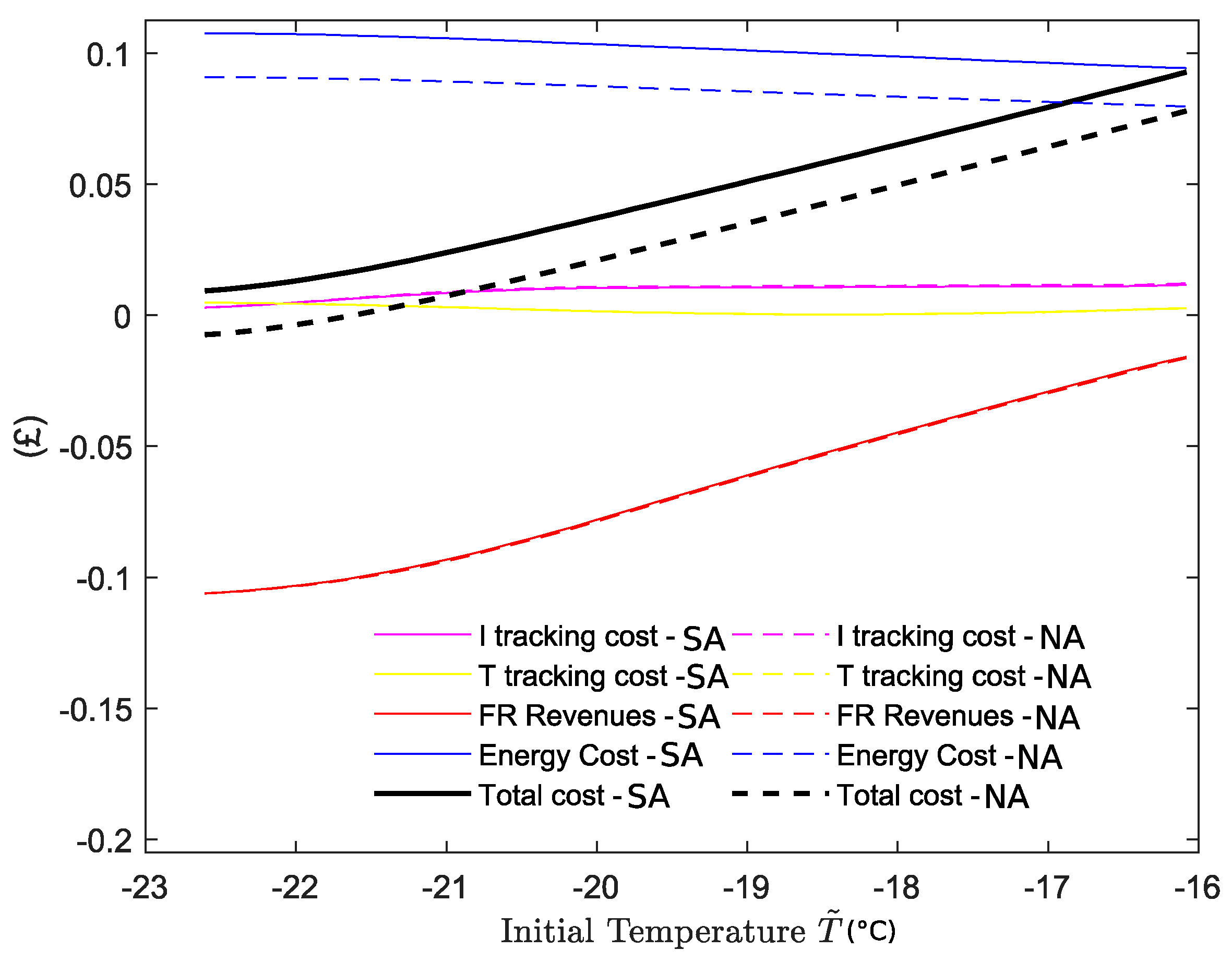
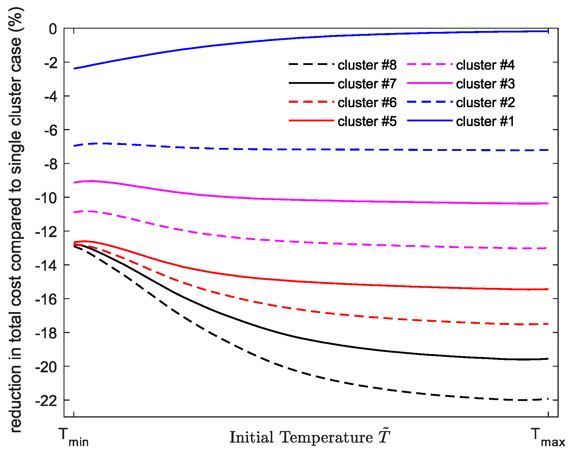
4.2.2. Assessing the Cost Components of Individual TCLs

Having discussed the aggregate impact of the TCLs population on the system through the quantities U S ( t ) , U N ( t ) , and R ( t ) , the focus moves now to the behavior of a single TCL in the NA and SA. Figure 7 shows the different components (as defined in Table 1) of the cost function (18) of the individual TCL, parametrized by its initial temperature T ( 0 ) = T ˜ . As anticipated in the context of Figure 6d, a TCL located in the NA faces lower total costs (dashed black) compared to a TCL in the SA (solid black). This result is motivated by the differences in the energy costs in the two cases, represented in the figure by the blue lines. On the other hand, since all the TCLs receive the same availability fee ρ ( t ) regardless of their geographical location, the revenues for FR allocation are almost the same in both areas (solid and dashed red lines).
As expected, the total cost is lower for TCLs with lower initial temperature. This follows from the monotonicity of λ ( T ) in (17) with respect to the temperature T : colder appliances will have the opportunity to allocate more FR during the night hours, i.e., when ρ ( t ) is higher, and therefore will receive higher FR revenues. Furthermore, it is worth noting that TCLs in the NA with lower T ˜ (almost up to −21 °C) would actually collect revenues to operate (and still maintain feasible internal temperatures) since the revenues from FR allocation exceed the energy cost component. Finally, the results in Figure 7 show that the impact of energy costs and FR revenues in (18) is significantly larger than the tracking terms (magenta and yellow lines).
It is interesting to note that the differences in costs for different initial temperatures introduce in the considered framework an additional gaming layer: the owners of the TCLs could further improve their objective function by ensuring that their devices reach a lower temperature at the beginning of the considered optimization time horizon. However, it should be emphasized that this element has a negligible impact on the overall equilibrium solution, for two reasons:
  • If all rational participants were to perform this change, the initial temperature distribution m 0 ( T ) would change significantly, thus leading to a different equilibrium solution for which the new values of initial temperature are potentially suboptimal.
  • In realistic contexts, the uncertainty and noise associated to the operation of the TCL would lead to a more diversified temperature distribution, thus reducing the impact of the initial temperature state on costs.
Besides the comparison of the TCLs cost breakdown between TCLs, it is worth assessing the total costs at both areas with respect to a Business as Usual (BaU) operation of the TCLs. In this case, single TCLs follow the regular hysteresis loop, switching OFF only when the minimum temperature T m i n is reached and switching ON only at T m a x . The aggregate TCL consumption under the BaU is U k B a U ( t ) = U k , 0   t [ 0 , t f i n ] and k = { S , N } and therefore is independent of energy prices, although the devices still have to sustain energy costs for their operation. Note that since TCLs do not currently provide flexibility services to the system, (i) the allocation of FR under the BaU is not enabled, with R B a U ( t ) = 0   t [ 0 , t f i n ] and (ii) TCLs do not collect any FR availability fee.
The ability to reach significant cost savings with the proposed DCS compared to the BaU is demonstrated in Figure 8, which shows the percentage variation in the total cost achieved with the DCS with respect to the BaU.
The TCLs in the NA with colder T ˜ are those that benefit the most compared to the BaU (−105% in costs), implying that they are able to achieve a net profit through the availability fee for FR. The minimum cost reduction (≈−55%) is obtained by TCLs in the NA with higher T ˜ , given their limited capability to exploit the new paradigm and provide FR in the early hours of the day.

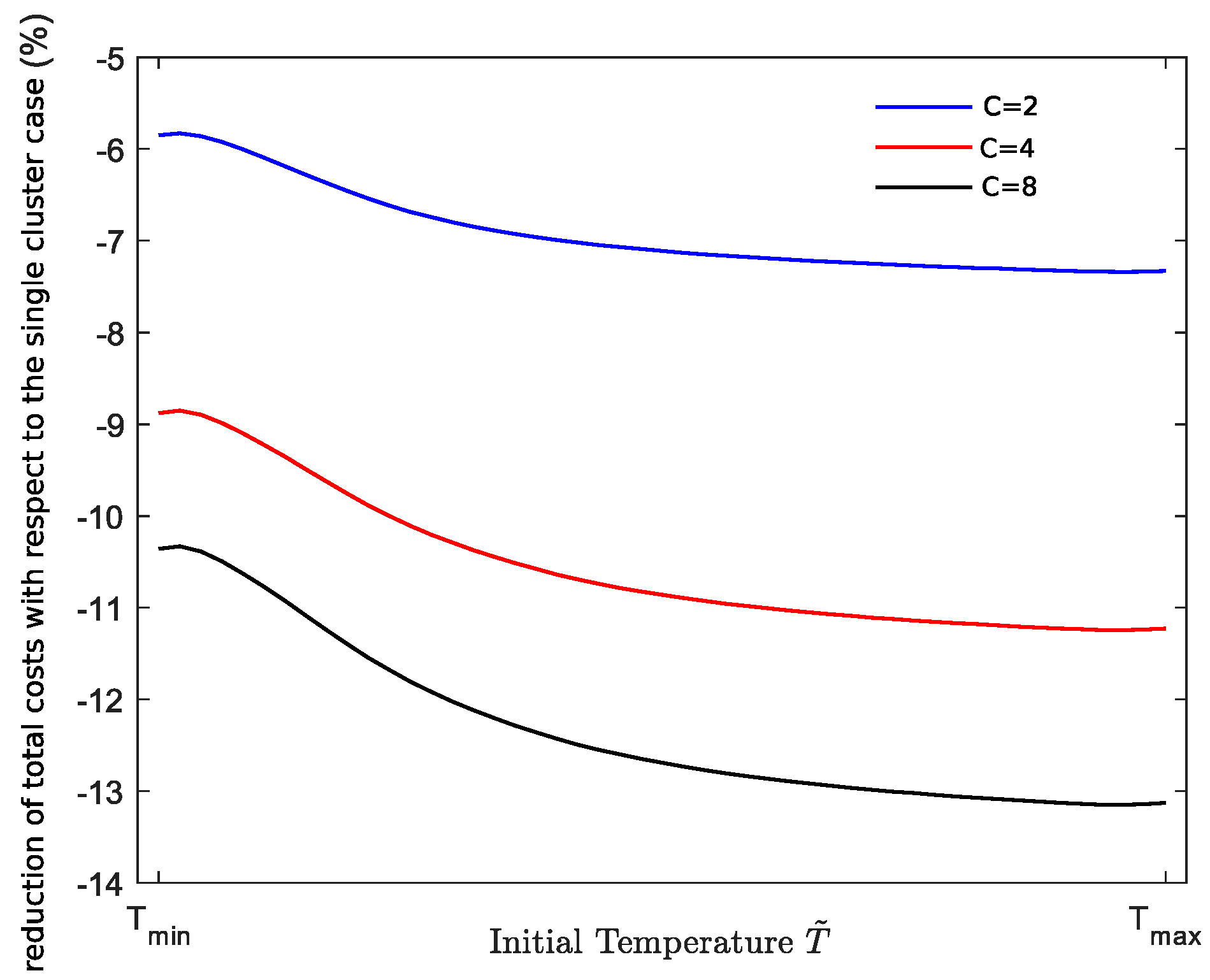
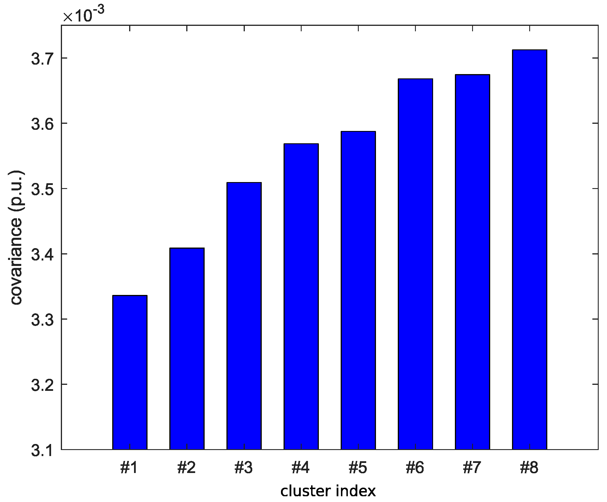
4.3. Impact of Clustering TCLs Populations

In this case study, the results obtained in the BC with the proposed control strategy are compared with three other scenarios where the TCL population is partitioned into two, four, and eight clusters, respectively ( C = 2, C = 4, and C = 8). The comparison focuses on the variation in the total costs faced by individual TCLs of each cluster with respect to the total cost sustained when the whole TCL population is described by same parameters ( C = 1).
The application of the clustering procedure described in Section 3.1 would let clusters of more efficient TCLs emerge compared to those described in a single cluster environment. In other words, as suggested in Figure 4 and in accordance with [6], the representative parameters of TCLs in certain clusters would, for instance, imply lower energy consumptions. This is the result, inter alia, of higher σ or lower π 0 , in turn induced for example by different temperature thresholds T m a x , T m i n , or different ζ . As general result, the overall steady state power consumptions U N , 0 and U S , 0 would decrease, causing the total costs faced by TCLs to follow the same trend. In order to avoid this trivial result, the number of TCLs in each cluster c (i.e., n N , c and n S , c for the NA and SA) were modified in order to maintain the same the steady state power consumptions in all the scenarios. In this way, we avoid the case of TCLs experiencing reduced total costs simply because p N ( t ) , p S ( t ) are lower since less generation is required and thus committed. All relevant parameters describing TCLs in each cluster are in Table A1 in Appendix A.
For simplicity, the results presented in this section refer to the case of TCLs in the SA, as similar trends can be identified in the NA. Simulation results show that the aggregate profiles U N ( t ) , U S ( t ) , and R ( t ) do not vary significantly when increasing the number of clusters from C   = 1 to C = 8. Similar outcomes arise considering p N ( t ) , p S ( t ) , and ρ ( t ) . The percentage cost reduction obtained with multiple clusters with respect to the case with C = 1 (i.e., the black solid line in Figure 7) is presented in Figure 9. Results were scaled up in order to align the values of T m i n and T m a x in each case.
The lines in Figure 9 indicate average costs, weighted by the number of TCLs in each cluster. In other words, the represented values indicate the expected total operating costs sustained by a TCL randomly selected among those in the SA and for a different initial temperature. Overall, the higher the total number of clusters C the lower the total energy costs will be. In other words, a more detailed model representation of the actual differences between the TCL parameters could provide significant economic benefits. Once again, we point out that the values of p N ( t ) , p S ( t ) , and ρ ( t ) did not vary significantly compared to the BC results, as we offset the simple implication that more efficient TCLs consume less, reduce the system prices, and thus sustain lower energy costs.
Results in Figure 9 provided general insights on the TCLs populations analyzed as a whole. The allocation of the total costs between TCLs different clusters in the same scenario, illustrated in Figure 10, allows to draw more specific conclusions. Results refer to the scenario with C   = 8 and show percentage variations compared to the same results obtained in DCS BC, i.e., with C   = 1. Once again, results were scaled to align T m i n and T m a x of each cluster.
The total costs for different intimal temperatures T ˜ vary significantly with respect to the BC for the TCLs in cluster #8 (reductions up to −22%, dashed black). On the contrary, there are marginal differences for the TCLs in cluster #1 (solid blue). In general, lower total costs follow from the ability of TCLs in clusters with higher index to modulate the power consumption (above and below the steady state level) and in turn allocate FR when reacting to the price signals p N ( t ) , p S ( t ) , and ρ ( t ) .
An indication of the link between total cost reduction and flexible power consumption is offered in Figure 11, where the covariances of U s , c ( t ) and the correspondent FR allocation ( R s , c ( t , U s , c )) are shown for each of the eight clusters. Note that amplitude of U s , c ( t ) and the correspondent FR allocation may vary noticeably among each cluster c = { 1 , C } due to different sizes of the clusters ( n s , c ). Hence, per unit values are adopted when calculating the covariances, using the steady-state consumptions of each cluster U s , c , 0 as base. It can be seen that the values of the covariance increase with the cluster index, thus showing the same trend as the percentage cost reduction in Figure 10.
Finally, increasing the number of clusters implies longer simulation times, although the number of iterations to converge to an equilibrium solution does not increase. In particular, the simulation times of the proposed DCS with are 35, 70, 150 min when C   = 2, C   = 4, and C = 8, respectively.

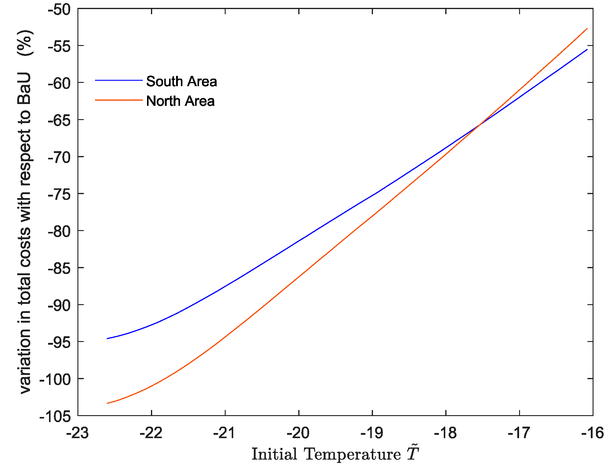
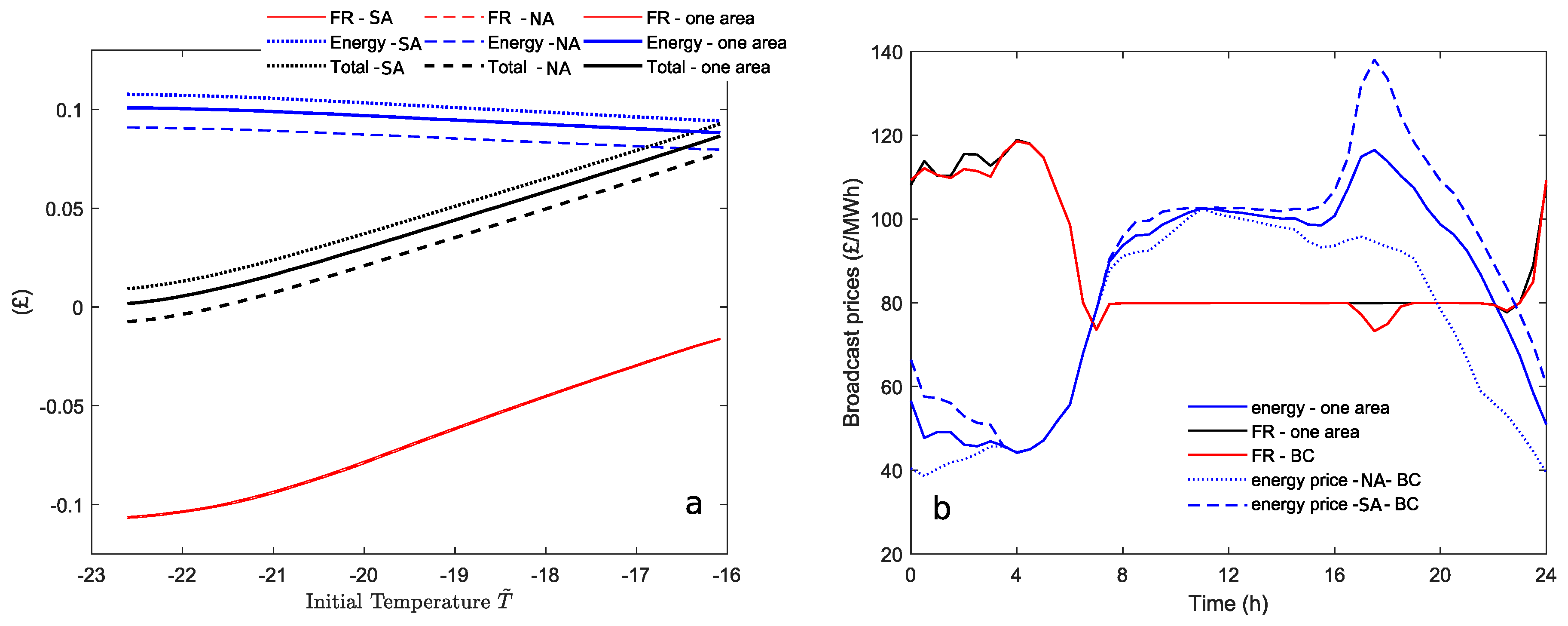
4.4. Multi-Area vs. Single-Area Scheduling

This section assesses the impact of the network constraints of the UC problem on TCLs total costs. The DCS scenario in the BC is thus compared to an alternative case where the upper/lower bounds on F ( t ) in (8) are removed. Note that neglecting the network topology, i.e., merging the two areas of the system in Figure 1 into a single, larger area, is a typical assumption in power system UC algorithms [23,28]. In this setup, p N ( t ) = p S ( t ) would hold t [ 0 , t f i n ] . The comparison of the TCLs cost breakdown is illustrated in Figure 12a, where the energy cost component is in blue, the FR revenues in red, and the total cost in black. To preserve the clarity of the picture, minor cost components such as the tracking components of I ( t ) and T ( t ) are not included. Moreover, solid lines refer to the one-area scheduling approach, whereas the dashed and dotted lines refer to the NA and SA in the DCS BC, respectively.
The analysis of Figure 12a indicates that, in the case of a single area, TCLs in the NA would face higher total costs. There is an opposite trend for the TCLs in the SA that would instead benefit from a one-area scheduling approach. These variations follow from similar changes in the energy costs (blue lines). The revenues associated to FR allocation instead do not show noticeable differences, as inferable from the three overlapped red lines. The cost variations can be justified by a comparison of the relevant price signals, presented in Figure 12b. Besides the time periods t with equal prices in the BC case, the energy prices p N ( t ) and p S ( t ) are, respectively, lower and greater than the energy price (single quantity) in the one-area scenario. On the other hand, only small differences are registered when comparing the FR prices (solid black line with the one-area approach and solid red line referring to the BC setup). The comparison of the aggregate power profiles U N ( t ) ,   U s ( t ) , and R ( t ) confirm the results discussed above.

5. Conclusions

This paper proposed a novel priced-based distributed coordination method for populations of TCLs that explicitly interact with the commitment/dispatch decisions and the security of multi-area power systems. In particular, the TCL coordination is obtained through a mean field game formulation which is combined with the optimal scheduling algorithm of a two-area power system.
The proposed method was proved to converge to an equilibrium solution which enables TCLs to individually optimize their energy consumption and corresponding FR allocation in response to a set of area-dependent price signals derived from the UC.
Moreover, the formulation accounts for the intrinsic heterogeneous nature of large TCLs populations. Firstly, this work showed how to partition the ensemble of devices into clusters of TCLs with similarities in the parameters’ space. Secondly, the population clustering was included in the mean field game formulation, with no relevant increase in computational complexity. Finally, the effectiveness of the distributed coordination method was proved through simulations evaluating its economic benefit with respect to the properties of the TCLs in each cluster.
Further work will extend the current power system modeling and mean field game formulation to increase the number of price signals and include additional ancillary services (e.g., enhanced frequency response, high frequency response, and secondary response) characterized by different delivery time and commitment patterns. For instance, the provision of high frequency response would require a TCL being off and then switched on for a certain amount of time, decreasing its internal temperature. This is opposite to the primary response investigated in this work, which needs a TCL to be on and then switched off, increasing its internal temperature. Moreover, the provision of secondary frequency response requires larger thermal energy reservoirs since a TCL delivering this service is kept off for several minutes. Interactions between TCLs and other forms of domestic storage and sources of generation will also be explored, aiming to implement a more effective energy arbitrage that makes use of storage capacity or local renewable generation to overcome the power consumption limitations of the TCLs due to their thermal constraints. As an example, future work will investigate potential cost reductions for TCLs scheduling their operational patterns based on the time-dependent availability of “zero-cost” energy provided by local photovoltaic generation. This feature would not only simply reduce the energy-related cost, but it would also help TCLs to better manage the internal energy buffer employed to the provision of a portfolio of frequency services.

Author Contributions

Conceptualization, V.T., A.D.P. and G.S.; methodology, V.T. and A.D.P.; software, V.T. and A.D.P.; validation, V.T., A.D.P. and G.S.; formal analysis, V.T. and A.D.P.; investigation, V.T. and A.D.P.; resources, G.S.; data curation, V.T. and A.D.P.; writing—original draft preparation, V.T. and A.D.P.; writing—review and editing, V.T. and A.D.P.; visualization, V.T. and A.D.P.; supervision, G.S. All authors have read and agreed to the published version of the manuscript.

Funding

The authors are grateful for the valuable support and funding received by the UK EPSRC project “Integrated Development of Low-Carbon Energy Systems” (IDLES, Grant EP/R045518/1).

Conflicts of Interest

The authors declare no conflict of interest.

Nomenclature

Acronyms
ACAlternating current
BaUBusiness as usual
BCBase case
CCGTCombined cycle gas turbine
DCSDistributed coordination strategy
FRFrequency response
GBGreat Britain
HVDCHigh voltage direct current
NNorth
NANorth area
OCGTOpen cycle gas turbine
PDEPartial differential equation
RoCoFRate of change of frequency
SSouth
SASouth area
TCLThermostatically Controlled Load
UCUnit commitment
Indices
g Index of generation technology
k Index of system area
c Index of TCL cluster
l Index of linearization cuts
Parameters
a k , g No-load cost of generation technology g in area k (£/MWh)
ε k , g Linear cost of generation technology g in area k (£/MWh)
η k , g Quadratic cost of generation technology g in area k (£/MW2h)
χ k , g Headroom for FR of generation technology g in area k
s k , g FR slope of generation technology   g in area k
P k , g m a x Installed capacity of generation technology g in area k (MW)
θ Maximum infeed loss (MW)
D Load damping (Hz-1)
f m a x Maximum frequency deviation (Hz)
f q s s Quasi-steady-state frequency limit (Hz)
f r f Frequency deviation for RoCoF (Hz)
t r f Time interval for RocoF (s)
t d Delivery time for FR (s)
f 0 Nominal frequency (Hz)
h k , g Constant of inertia of generation technology g in area k (s)
h θ Constant of inertia of infeed generation loss (s)
σ c Thermal time constant of TCL in cluster c (h)
T o f f , c Ambient temperature of TCL in cluster c (°C)
T m a x , c Maximum temperature of TCL in cluster c (°C)
T m i n , c Minimum temperature of TCL in cluster c (°C)
T o n , c Asymptotic cooling temperature of TCL in cluster c (°C)
ζ c Heat exchange parameter of TCL in cluster c (W/°C)
π 0 ,   c Duty cycle of TCL in cluster c
Γ c TCL power in cluster c (W)
t f i n Time horizon (h)
n k , c Number of TCLs in area k and cluster c
T ¯ Target temperature (°C)
α Discomfort cost parameter (£/h(°C)2)
β Antisynchronization cost parameter (£/h(°C)2)
U k , c Aggregate TCL steady state power in area k and cluster c (MW)
C Number of clusters of TCLs
F m a x Interconnector’s capacity (MW)
μ Commitment parameter
n l Number of linearization cuts
X Set of TCLs’ parameters
γ Number of TCLs’ parameters used for clustering
Ω c Set of TCLs in cluster c
δ c Mean of TCLs’ parameters in cluster c
Functions
p k ( · ) Energy price in area k (£/MWh)
ρ ( · ) FR price in area k (£/MWh)
U k ( · ) Aggregate TCL power in area k (MW)
U k , c ( · ) Aggregate TCL power in area k and cluster c (MW)
R ( · ) Aggregate FR from TCLs (MW)
ξ k ( · ) Set of generation decision variables in areas k
F ( · ) Power flow through the interconnector (MW)
H g , k ( · ) Commitment level of generation technology g in area k
P g , k ( · ) Dispatch level of generation technology g in area k (MW)
Π g , k ( · ) FR from generation technology g in area k (MW)
φ ( · , · , · ) Minimized total generation costs per unit of time (£/h)
L k ( · ) Inflexible load in area k
H ^ ( · ) System post-fault inertial response (MWs2)
R ^ ( · ) System FR allocation (MW)
q ^ ( · ) Nadir constraint requirement function (MWs) 2
T ( · ) Internal temperature of TCL (°C)
I ( · ) Temperature variation of TCL (°C)
u k , c ( · ) Power consumption of TCL in area k and cluster c (W)
( · ) TCL temperature dynamics (°C/s)
λ ( · ) Fraction of TCL power consumption allocated as FR
r k , c ( · ) Allocated FR of TCL in area k and cluster c (W)
J ( · ) Cost function of TCL (£)
I ¯ ( · ) Target temperature variation (°C)
Ψ ( · ) Terminal cost function (£)
V k , c ( · ) Value function for cost-minimization of TCL in area k and cluster c (£)
u N , c * ( · ) Optimal feedback control of TCL in area k and cluster c (W)
m k , c ( · ) State distribution of TCLs in area k and cluster c

Appendix A

Table A1. Characteristics of TCLs.
C T m a x   [ ° C ] T m i n   [ ° C ] T o f f   [ ° C ] ζ σ n S , c n N , c
1−16.08−22.6121.980.884.559,557,3751,686,596
2−14.58−20.5820.170.954.543,332,505588,089
−16.08−22.6121.980.884.558,854,9451,562,637
4−14.01−20.1119.340.984.525,980,1911,055,328
−15.01−21.1620.720.934.565,776,7601,019,428
−14.70−20.7320.210.964.544,193,085739,956
−16.09−22.5921.980.884.553,250,781573,667
8−14.76−20.7319.870.954.541,016,350179,356
−13.57−19.7518.880.994.572,606,425459,957
−15.45−21.7221.140.914.553,266,268576,400
−14.73−20.8020.390.944.562,160,742381,307
−14.03−20.1319.310.984.553,110,704548,948
−15.06−21.2120.750.934.561,431,354252,592
−16.09−22.5721.990.884.552,886,580509,396
−14.42−20.4519.590.974.589,557,3751,686,596

Appendix B

This section presents additional system-level results obtained with the DCS under the BC framework. Figure A1a,b shows the optimal generation mix as solution of the UC problem in the SA and NA, respectively. The nuclear technology (blue area) acts as base load generation source in both areas. The energy flowing through the interconnectors (cyan area) is used to supply the load of the SA (Figure A1a) as it is below the dashed black line representing the local system demand L s ( t ) + U s ( t ) . Clearly, in the NA (Figure A1b), the energy through the interconnectors is in excess of the local demand. From the analysis of Figure A1a it is also possible to infer that the interconnectors are always fully loaded (7000 MW) with minor exceptions between 04:00 and 07:00 am, in accordance with the results in Figure 6d. It is worth noting that the cyan area in Figure A1b is a mix of wind energy (green area), CCGT energy (red area), and OGCT energy (grey area) supplied by the corresponding generation technologies in the NA.
Figure A1. (a) Generation mix in the SA. (b) Generation mix in the NA. (c) Available wind generation in the NA and SA. (d) Percent generation commitment levels in the NA and SA.
Energies 13 06483 g0a1
The available wind profiles at both areas are shown in Figure A1c. A smoother profile is reported in the SA (green dashed), whereas the NA experiences a large wind output variability (green solid) over the optimization horizon (24 h). Finally, Figure A1d illustrates the generation commitment level expressed in percentage of the maximum installed capacity. The chart indicates that all the wind generation is integrated. Similarly, the optimized system solution brings online all the available nuclear and CCGT generation. Since OCGT is the most expensive technology, the commitment levels are lower.

References

  1. Brouwer, A.S.; van den Broek, M.; Zappa, W.; Turkenburg, W.C.; Faaijac, A. Least-cost options for integrating intermittent renewables in low-carbon power systems. Appl. Energy 2016, 161, 48–74. [Google Scholar] [CrossRef] [Green Version]
  2. National Grid. Electricity Ten Year Statement (ETYS). 2019. Available online: https://www.nationalgrideso.com/research-publications/electricity-ten-year-statement-etys (accessed on 28 October 2020).
  3. Siano, P.; Sarno, D. Assessing the benefits of residential demand response in a real time distribution energy market. Appl. Energy 2016, 161, 533–551. [Google Scholar] [CrossRef]
  4. Zehir, M.A.; Batman, A.; Bagriyanik, M. Review and comparison of demand response options for more effective use of renewable energy at consumer level. Renew. Sustain. Energy Rev. 2016, 56, 631–642. [Google Scholar] [CrossRef]
  5. Wang, P.; Wu, D.; Kalsi, K. Flexibility Estimation and Control of Thermostatically Controlled Loads with Lock Time for Regulation Service. IEEE Trans. Smart Grid 2020, 11, 3221–3230. [Google Scholar] [CrossRef]
  6. Trovato, V.; Tindemans, S.; Strbac, G. Leaky storage model for optimal multi-service allocation of thermostatic loads. IET Gener. Transm. Distrib. 2016, 10, 585–593. [Google Scholar] [CrossRef] [Green Version]
  7. Conte, F.; Massucco, S.; Silvestro, F.; Ciapessoni, E.; Cirio, D. Stochastic modelling of aggregated thermal loads for impact analysis of demand side frequency regulation in the case of Sardinia in 2020. Int. J. Electr. Power Energy Syst. 2017, 93, 291–307. [Google Scholar] [CrossRef]
  8. Callaway, D.S.; Hiskens, I.A. Achieving controllability of electric loads. Proc. IEEE 2011, 99, 184–199. [Google Scholar] [CrossRef] [Green Version]
  9. Hao, H.; Sanandaji, B.M.; Poolla, K.; Vincent, T.L. Aggregate flexibility of thermostatically controlled loads. IEEE Trans. Power Syst. 2015, 30, 189–198. [Google Scholar] [CrossRef]
  10. Song, M.; Gao, C.; Shahidehpour, M.; Li, Z.; Yang, J.; Yan, H. State space modeling and control of aggregated TCLs for regulation services in power grids. IEEE Trans. Smart Grid 2019, 10, 4095–4106. [Google Scholar] [CrossRef]
  11. Singh, K.; Padhy, N.P.; Sharma, J. Influence of price responsive demand shifting bidding on congestion and lmp in pool-based day-ahead electricity markets. IEEE Trans. Power Syst. 2011, 26, 886–896. [Google Scholar] [CrossRef]
  12. Papadaskalopoulos, D.; Strbac, G. Nonlinear and randomized pricing for distributed management of flexible loads. IEEE Trans. Smart Grid 2016, 7, 137–1146. [Google Scholar] [CrossRef] [Green Version]
  13. Gu, C.; Yan, X.; Yan, Z.; Li, F. Dynamic pricing for responsive demand to increase distribution network efficiency. Appl. Energy 2017, 2015, 236–243. [Google Scholar] [CrossRef] [Green Version]
  14. Li, S.; Zhang, W.; Lian, J.; Kalsi, K. Market based coordination of thermostatically controlled loads—part i: A mechanism design formulation. IEEE Trans. Power Syst. 2016, 31, 1170–1178. [Google Scholar] [CrossRef]
  15. Gan, L.; Topcu, U.; Low, S.H. Optimal decentralized protocol for electric vehicle charging. IEEE Trans. Power Syst. 2013, 28, 940–951. [Google Scholar] [CrossRef] [Green Version]
  16. Ma, Z.; Callaway, D.; Hiskens, I. Decentralized charging control of large populations of plug-in electric vehicles. IEEE Trans. Control Syst. Technol. 2013, 21, 67–78. [Google Scholar] [CrossRef]
  17. Grammatico, S. Dynamic control of agents playing aggregative games. IEEE Trans. Autom. Control 2017, 62, 4537–4548. [Google Scholar] [CrossRef] [Green Version]
  18. De Paola, A.; Angeli, D.; Strbac, G. Price-based schemes for distributed coordination of flexible demand in the electricity market. IEEE Trans. Smart Grid 2017, 8, 3104–3116. [Google Scholar] [CrossRef]
  19. Lasry, J.; Lions, P. Mean field games. Jpn. J. Math. 2007, 2, 229–260. [Google Scholar] [CrossRef] [Green Version]
  20. Huang, M.; Caines, P.E.; Malhamé, R.P. Large population stochastic dynamic games: Closed-loop mckean-vlasov systems and the nash certainty equivalence principle. Commun. Inf. Syst. 2006, 6, 221–252. [Google Scholar]
  21. Bauso, D. Dynamic demand and mean field games. IEEE Trans. Autom. Control 2017, 62, 6310–6323. [Google Scholar] [CrossRef] [Green Version]
  22. Kizilkale, A.C.; Salhab, R.; Malhamé, R.P. An integral control formulation of mean field game based large scale coordination of loads in smart grids. Automatica 2019, 100, 312–322. [Google Scholar] [CrossRef] [Green Version]
  23. De Paola, A.; Trovato, V.; Angeli, D.; Strbac, G. A Mean Field Game Approach for Distributed Control of Thermostatic Loads Acting in Simultaneous Energy-Frequency Response Markets. IEEE Trans. Smart Grid 2019, 10, 5987–5999. [Google Scholar] [CrossRef]
  24. Trovato, V.; Sanz, I.M.; Chaudhuri, B.; Strbac, G. Advanced Control of Thermostatic Loads for Rapid Frequency Response in Great Britain. IEEE Trans. Power Syst. 2017, 32, 2106–2117. [Google Scholar] [CrossRef] [Green Version]
  25. Papadaskalopoulos, D.; Strbac, G. Decentralized participation of flexible demand in electricity markets—Part I: Market mechanism. IEEE Trans. Power Syst. 2013, 28, 3658–3666. [Google Scholar] [CrossRef]
  26. Chen, H.; Liu, M.; Cheng, Y.; Lin, S. Modeling of Unit Commitment with AC Power Flow Constraints Through Semi-Continuous Variables. IEEE Access 2019, 7, 52015–52023. [Google Scholar] [CrossRef]
  27. Chau, T.K.; Yu, S.S.; Fernando, T. Novel Control Strategy of DFIG Wind Turbines in Complex Power Systems for Enhancement of Primary Frequency Response and LFOD. IEEE Trans. Power Syst. 2018, 33, 1811–1823. [Google Scholar] [CrossRef]
  28. Trovato, V.; Bialecki, A.; Dallagi, A. Unit commitment with inertia-dependent and multispeed allocation of frequency response services. IEEE Trans. Power. Syst. 2019, 34, 1537–1548. [Google Scholar] [CrossRef]
  29. Teng, F.; Trovato, V.; Strbac, G. Stochastic Scheduling with Inertia-Dependent Fast Frequency Response Requirements. Ieee. Trans. Power Syst. 2016, 31, 1557–1566. [Google Scholar] [CrossRef] [Green Version]
  30. Bertsekas, D.P. Dynamic Programming and Optimal Control, 2nd ed.; Athena Scientific: Belmont, MA, USA, 2000. [Google Scholar]
  31. MacQueen, J.B. Some Methods for classification and Analysis of Multivariate Observations. Proc. Berkeley Symp. Math. Statist. Prob. 1967, 1, 281–297. [Google Scholar]
  32. MathWorks. k-Means Clustering. Available online: https://uk.mathworks.com/help/stats/kmeans.html#buefthh-3 (accessed on 28 October 2020).
Figure 1. Schematics of the two-areas power system model.
Energies 13 06483 g001
Figure 2. Diagram of the interactions between the Thermostatically Controlled Loads (TCLs) at each area and the unit commitment.
Energies 13 06483 g002
Figure 3. Interactions between ancillary services and conditions on the dynamic evolution of frequency following a sudden, large infeed loss.
Energies 13 06483 g003
Figure 4. Illustrative example of partitioning a population of heterogeneous TCLs in four clusters.
Energies 13 06483 g004
Figure 5. (a) Total power consumptions U S ( t ) at different iterations of the Distributed Coordination Strategy (DCS). (b) Zoom of U S ( t ) on a smaller time interval. (c) Total power consumptions U N ( t ) at different iterations of the DCS. (d) Total response allocation R ( t ) at different iterations of the DCS. The iteration number is indicated by the superscript in brackets.
Energies 13 06483 g005
Figure 6. (a) Energy prices p S ( t ) in the SA at different iterations of the DCS. (a,b) Energy prices p N ( t ) in the NA at different iterations of the DCS. (c) System-level FR prices ρ ( t ) at different iterations of the DCS. (d) p S ( t ) , p N ( t )
Energies 13 06483 g006
Figure 7. Breakdown of costs in (18) as function of initial temperature T ˜ of single TCL in the NA (dashed) and in the SA (solid). Black lines for total costs, blue for energy costs, red for FR fees, yellow for T -tracking and magenta for I -tracking cost.
Energies 13 06483 g007
Figure 8. Percentage variation of the total cost (18) achieved with the proposed DCS with respect to the Business as Usual (BaU).
Energies 13 06483 g008
Figure 9. Percent reduction in total costs for individual TCLs when the TCL population in partitioned in C   = 2 (blue), C   = 4 (red), and C = 8 (black) clusters with respect to the case when C = 1
Energies 13 06483 g009
Figure 10. Percentage reduction in total cost for individual TCLs in different clusters compared to the total cost sustained when C   = 1 (Base Case (BC) assumptions).
Energies 13 06483 g010
Figure 11. Covariance of the aggregate cluster consumption U s , c ( t ) and corresponding FR allocation R s , c ( t , U s , c )) expressed in per unit of the steady-state level U s , c , 0 for different clusters c = { 1 , , 8 }
Energies 13 06483 g011
Figure 12. (a) Cost breakdown for individual TCLs with different intimal temperature T ˜ . Solid lines refer to the UC scheduling with a one area approach. (b) Energy prices and FR prices at the equilibrium solution. Dashed and dotted lines refer to the DCS BC for the NA and SA, respectively.
Energies 13 06483 g012
Table 1. Description of the terms of the TCL cost function J k   (18).
Term in J k Description
p k ( t ) u k ( t ) Electricity Cost: the instantaneous cost associated to the power consumption u k ( t ) . It depends on the area index k of the TCL, since p N ( t ) may differ from p S ( t ) .
ρ ( t ) r ( T ( t ) ,   u k ( t ) ) Response Revenue: the product of the availability fee   ρ ( t ) awarded for FR provision and the actual FR allocation of the TCL r ( T ( t ) ,   u k ( t ) ) .
α ( T ( t ) T ¯ ) 2 T tracking cost: discomfort term which penalizes quadratically, through the cost parameter α , the deviations from a target temperature T ¯ .
β ( I ( t ) I ¯ ( t ) ) 2 I tracking cost: quadratic cost parameterized by β   that penalizes the deviations of I ( t ) from a set-point I ¯ ( t ) . This antisynchronization term allows to diversify the behavior of groups of TCLs that have reached the same temperature T ( t ) from different initial values T ˜ and therefore have different values of I ( t ) .
Ψ ( I ( t f i n ) ) Terminal cost function: a periodic constraint is enforced by choosing Ψ ( I ) = Λ · I 2 and penalizing quadratically the final value I ( t f i n ) = T ( t f i n ) T ˜ , i.e., the difference between final and initial temperature of the TCL.
Table 2. Generation characteristics.
NuclearCCGTOCGTWind
Installed capacity P g , k m a x [MW]5000/100025,000/700025,000/700010,000/20,000
No-load cost a k , g [£/MWh]0/024/732/100/0
Production cost ε k , g [£/MWh]1/150/55100/1051/1
Production cost η k , g [£/MW2h]0.0009/0.00090.01/0.0120.02/0.0220.001/0.001
Constant of inertia h g , k [s]6/64/44/4-/-
FR headroom χ g , k -/-0.1/0.10.1/0.1-/-
FR slope s g , k -/-0.4/0.40.5/0.5-/-
Publisher’s Note: MDPI stays neutral with regard to jurisdictional claims in published maps and institutional affiliations.

