Article

How Strategic Behavior of Natural Gas Exporters Can Affect the Sectors of Electricity, Heating, and Emission Trading during the European Energy Transition

Chair for Management Science and Energy Economics, University of Duisburg-Essen, D-45127 Essen, Germany
Energies 2020, 13(19), 5040; https://doi.org/10.3390/en13195040
Submission received: 30 June 2020 / Revised: 10 August 2020 / Accepted: 13 August 2020 / Published: 24 September 2020
(This article belongs to the Special Issue Model Coupling and Energy Systems)

Abstract

:
The European demand for natural gas imports may change through the energy transition, which may affect natural gas exporters’ strategic behavior and consequently the natural gas prices. Changes in natural gas prices in turn influence the European energy sector in terms of gas consumption in the short-term and investments in the long-term. The present paper develops a large-scale partial equilibrium market model formulated as a mixed complementarity model (MCP) with conjectural variations. This model considers the global natural gas market and the European markets of electricity, heating, and emission trading in one equilibrium. We apply this model to investigate the long-term impact of market power by gas exporters on the mentioned energy-related markets on the horizon of 2050. The results of the study show that a decrease in the market power by gas exporters decreases natural gas prices, leading to cheaper electricity and CO2 prices in the mid-term. However, a very tight emission cap in 2050 can result in the reverse phenomenon.

1. Introduction

Natural gas is considered to maintain its role in European energy consumption during the energy transition in the mid-term [1]. Consequently, changes in the natural gas sector can affect gas-consuming sectors and vice versa. On the one hand, European carbon abetment policies aim to shift energy consumption and investments towards renewables and less carbon-intense fuels such as natural gas. This shift may affect the European gas demand and therefore affect the natural gas prices. On the other hand, an increase in natural gas prices may affect gas-consuming sectors in terms of gas consumption in the short-term and investment patterns in the long-term. Thus, studying the interdependencies between the natural gas sector and gas consumer sectors (e.g., power sector) is of great interest.
Particularly, among the natural gas-consuming sectors, the power and heating sectors are significant consumers. These sectors also have great potential to undergo considerable changes during the European energy transition. Accordingly, studying the interactions between the natural gas sector and the power and heating sectors is of high relevance. The present paper aims to investigate the interdependencies between the natural gas sector and the sectors of electricity, heating, and emission trading during the European energy transition. Among the cross-sectoral uncertainties, we focus on the effect of strategic behavior by the natural gas producers and its influence on the other sectors.
It is notable to mention that the European gas supply highly depends on imports. According to BP Statistical Review of World Energy [2], almost 60% of the European gas demand is covered through imports in 2018. Pipelines hold a share of 78% in the total imported gas. As most EU members depend on a few suppliers and transport routes, disruption caused by political disputes [3] can endanger the security of supply. To mitigate the risk, the EU has introduced the “The security of gas supply regulation” [4]. But even if risk of gas supply interruption may be mitigated, a limited number of suppliers may induce higher prices and corresponding welfare losses in the EU.
There are numerous literature sources that discuss the role of different technologies, such as EVs, hydrogen, power-to-heat, etc. for the European energy transition. Jimenez-Navarro et al. [5] examined the role of centralized cogeneration plants in the future decarbonized energy system. Roach and Meeus [6] developed a partial equilibrium model for the power and gas sectors to analyze future investments, whereas Emosnt et al. [7] focused on the hydrogen infrastructure. Pavičević et al. [8] combined a long-term planning tool with a unit commitment model of power markets. Although they considered multiple sectors in their analysis, they neither considered the natural gas markets nor modeled the effect of strategic behavior. Brown et al. [9] discussed the coupling of electricity to other energy sectors, such as transport and heating, and investment in transition networks, whereas Steinmann et al. [10] focused on storage technologies (PtH, etc.) as a way to achieve the sector coupling. While many of these studies focus on one or two aspects of sector coupling, they miss the linkage with the natural gas sector.
The interdependencies between the natural gas sector and other sectors have been studied previously in some literature [11,12,13,14,15]. In [12], Erdener et al. investigated the gas dependency of gas-fired power plants in the electricity system as well as the electric dependency of electric-driven compressors in the gas system. In [14], Deane et al. developed an integrated energy model for the EU 28 to examine the security of supply. Hauser P. et al. [15] combined an optimization model of heat and electricity with a natural gas network model to study gas network congestion resulted by the increasing electricity demand. These studies formulate the natural gas sector as an optimization model. Although the optimization approach has advantages in modeling natural gas networks as well as using detailed data, it seems to be inefficient at describing the natural gas prices.
Apart from them, complementary models are used to formulate energy markets equilibria [16], [17]. The benefit of this approach while studying the natural gas market is their ability to consider strategic behavior [18,19]. The authors of [20,21] used complementarity-based approaches to investigate the interdependencies between the sectors of power, emission and natural gas.
Sppiecker [20] modeled the electricity, natural gas and emissions trading markets with simplified data to study the impact market power by natural gas producers on the power sector. Weigt [21] used an MCP model of combined natural gas and electricity markets to analyze different pathways for the long-term European decarbonization. However, their model neither considers the sectors of heating and emission trading nor analyzes the effect of strategic behavior by natural gas producers. Besides, cogeneration and the heating market are not studied widely with complementarity previously in academia. Virasjoki et al. [22] delivered an MCP formulation for CHP plants. They analyzed CHP producers’ roles in integrated markets but did not take into account other sectors.
Consequently, previous studies do not comprehensively describe the interdependencies between the natural gas market, the power market, the heating markets, and the emission trading market. To describe the comprehensive interactions of these markets, we develop an equilibrium model of natural gas, electricity, heating, and emission trading markets, using a mixed complementarity problem approach. For the heating and electricity markets, we deliver the heating markets, including the cogeneration of power and heat, power-to-heat, and heat boilers. We also consider endogenous investments in renewables. For the case study, we use real data of annual demand and available production capacities instead of stylized data to investigate how strategic behavior in the natural gas sector can affect consumption and investments in the power, heat, and emission trading sectors during the European energy transition. We believe the present work contributes to the existing sector coupling literature by providing a complex model that enables the study of the effect of market power in one sector on the other sectors. Besides, the current formulation can be extended to analyze strategic behavior in any of these sectors. It can be especially relevant for the heating sector, where the strategic behavior can influence the local markets in the future works.
The rest of this paper is structured as follows. Section 2 develops the mathematical formulation. Section 3 provides the data assumption and study design. Section 4 discusses the results. Section 5 concludes.

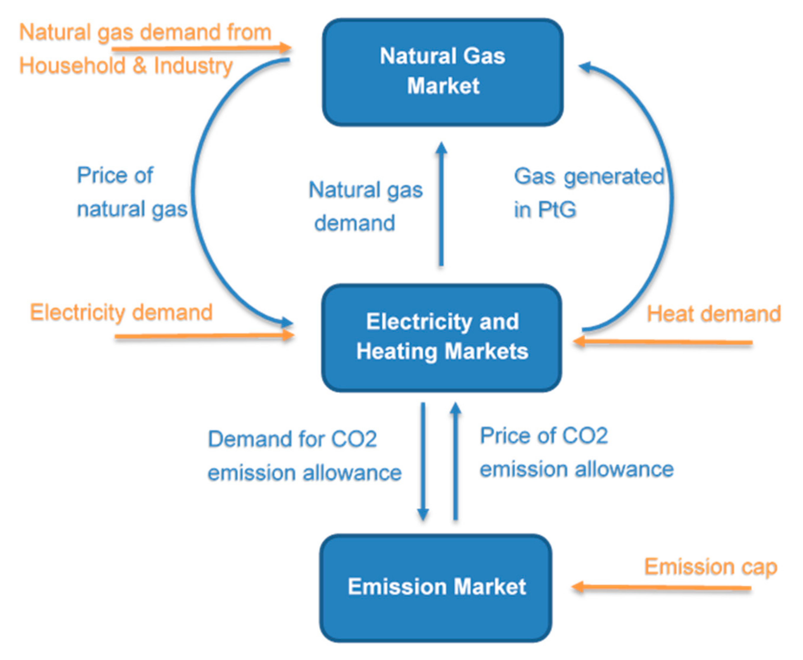
2. Theoretical Framework

The CELGEM (Complementarity Electricity Gas Emission Market) model presented in this paper, takes as a starting point the model developed in [23]. The model is a large-scale partial market equilibrium model based on the principles of Cournot–Nash equilibria (cf. Figure 1). Comparing the present version of the model with the earlier versions, we make considerable changes in the formulation of the electricity market and emission markets by adding endogen investment equations for renewables and integrating the heating sector. However, the mathematical formulation for the natural gas market remains the same. Therefore, in the rest of this section, we briefly explain the natural gas part, while delivering a detailed formulation for other sectors.

2.1. Natural Gas Market

As mentioned above, we do not change the formulation of the natural gas market. The equations of the natural gas market are the same as those published in [20]. We avoid republishing them in the present work and deliver a brief description explanation instead. In the gas part of the CElGEM-Model, market players are considered at three levels: producers and their associated traders (upstream), TSOs and shippers (midstream), and gas hubs (downstream). Producers operate their extraction equipment and supply their associated traders. Traders deal gas at different hubs as wholesale markets, where final demand is aggregated to three sectors of power and heating, industry, and residential. Demand curves are considered in each sector separately. The demand for natural gas in the power and heating sectors is determined endogenously by the power and heating markets. Gas pipelines, LNG shipping, and the corresponding terminals are considered as transport means. Storage operators run their facilities based on price signals of the market. Since political decisions considerably drive investments in the gas sector, we model the capacity investments exogenously.
The producers with their associated traders in the upstream and midstream layers choose their strategy taking into consideration that other players also follow their optimal strategy to maximize their profits. TSOs are assumed to be perfectly regulated, and, for shippers and the downstream layer, perfectly competitive markets are assumed. Yet, Traders (and their related producers) are assumed to exert market power and they may affect the market price through their supply of gas on hubs. The other players are considered as price-takers. For this modeling of the oligopolistic behavior of the natural gas market, the model uses the approach of conjectural variations [24]. In this approach, we introduce a mark-up factor, which determines the (assumed) degree of market power. This factor can vary from 0 (perfect competition or no market power) to 1 (full market power as in a Cournot-Nasholigopoly). In reality, the exercise of market power in the natural gas market is limited through various factors, including long-term contracts, political interferences, and market entry threats. Therefore, mark-up factors are set exogenously for each model run.

2.2. Electricity and Heat Producers

The electricity market has three levels of players, namely producers, transmission system operators (TSOs), and consumers, whereas for the heating market we consider the two levels of producers and consumers and do not consider heating networks.
The power and heat producers include CHP plants, non-CHP plants, renewables, heat boilers, and power-to-heat (PtH). Among the CHP power plants that produce electricity and heat, the technology classes of backpressure and extraction may be distinguished (e.g., used in [19,25]). Condensing plants by contrast can only generate electricity. Backpressure and extraction plants can produce electricity and heat simultaneously, whereas condensing plants can only generate electricity. Backpressure units are characterized by having one degree of freedom in terms of simultaneous production of heat and electricity whereas extraction units have two degrees of freedom. Simplified P-Q diagrams for these two types of CHP plants are shown in Figure 2. All the participants in the electricity and heating market maximize their profits in Equation (1). For the sake of simplicity and to save calculation time, we aggregate the producers to classes z based on their technology type, fuel type and technical properties. For each type of producers, q f , n , z , l E and q f , n , z , l H represent respectively the electricity and heat outputs in gas region f , electricity region n , and load segment l t . These energy outputs multiplied with the market prices for electricity λ f , n , z , l P E and district heating λ f , n , z , l P H yield revenues for producers. Total operational costs of each producer include a combination of the fuel cost F n , b z and the cost of CO2 emissions, divided by efficiencies, as well as other variable costs of operation, which are given by C n , z E ,   o t h for CHP and power generating units and C n , z H ,   o t h for heat-only units.
q f , n , z , l E q f , n , z , l H max   l D l ( q f , n , z , l E λ f , n , l P E + q f , n , z , l H λ f , n , l P H   ( F n , b z + β b z C O 2 λ C O 2 η f , n , z b k p . max , tot + η f , n , z r e s . max , e + η f , n , z O H max , th η f , n , z slope q f , n , z , l E ) ( q f , n , z , l E   + q f , n , z b k p . , l E / C f , n , z b k p . B + C f , n , z e x t . V q f , n , z e x t . , l H ) q f , n , z , l E C n , z E , o t h   q f , n , z O H , l H C n , z O H H , o t h λ f , n , l P E u f , n , l   A n n f , z O H L f , n , z O H P H , n e w )
In (1), η f , n , z b k p . m a x , t o t stands for the total efficiency (including power and heat) and is used for backpressure units only, whereas η f , n , z r e s . m a x , e is the electrical efficiency, which is used for the other electricity generators including condensing, extraction, and renewable plants. η f , n , z O H m a x , t h represents the thermal efficiency for heat-only units. Using a linear approximation, we also consider the change of efficiencies for thermal units (e.g., due to vintage effects) by introducing the slope parameter η f , n , z s l o p e [25,27]. Besides, the cost for CO2 emissions is calculated by multiplying the market price for CO2 allowance λ C O 2 with the fuel specific emission intensity factor β b z C O 2 . Unlike backpressure units, extraction CHP units can operate in the power-only mode and the cogeneration mode. We reflect this phenomenon in the total costs, by including C f , n , z e x t . V q f , n , z e x t . , l H and replacing the total efficiency with electrical efficiency. For backpressure units, the ratio of power to heat generation is fixed (cf. Figure 2). Therefore, we substitute the heat production q f , n , z , l H   with q f , n , z b k p . , l E / C f , n , z b k p . B to reduce the number of variables. We also model the operation of pump storages by including the cost for pumping λ f , n , l C E multiplied by the pumping amount u f , n , l .
Investments in each simulation year are calculated in a dynamic-recursive manner. We use myopic expectations for investments in new capacities. In this approach, new investments are determined based on the market equilibrium in each simulation year independent of the future simulation years. Accordingly, we expand the objective functions by the investment costs. The investment costs for power and CHP producers are obtained as the product of the additional electrical capacity L f , n , z P E , n e w and the annualized investment cost Ann z P E , n e w . Here, we consider a fixed power-to-heat ratio for new CHP units; hence, we can write the thermal capacity expansion as L f , n , z P H , n e w = L f , n , z P E , n e w C f , n , z B + C f , n , z V . we analyzed this ratio for ten new CCGT in Germany and found for all the plants the ratio to be close to 1.2. Similarly, for the heat-only units, the investment cost A n n f , z O H L f , n , z O H P H , n e w is based on the cost of additional thermal capacity.
Generally, the maximum electricity production of all producers is constrained to the maximum available electricity generation capacity. For the extraction units, the maximum electricity production must be within the feasible operating region, as illustrated in Figure 2. Therefore,
q f , n , z , l E ρ f , n , z , l E L f , n , z P E + L f , n , z P E , n e w 1 z Z e x t C f , n , z V q f , n , z , l H   :   ϑ f , n , z , l P E f , n , z , l
where ρ f , n , z , l E stands for the availability and L f , n , z P E stands for the maximum electricity generation capacity. To keep the outputs of extraction CHP producers in the feasible region, we also need the following equation:
q f , n , z , l E C f , n , z B q f , n , z , l H   : τ f , n , z , l P E f , n , z e x t . , l
For heat producers as well as CHP producers with extraction turbines, the heat generation also needs to be restricted by the maximum available heat generation capacity as follows:
q f , n , z , l H ρ f , n , z , l H L f , n , z P H + L f , n , z P H , n e w   : ϑ f , n , z , l P H f , n , z O H ,   e x t . , l
As the equations above represent a convex optimization problem, we can replace them with KKT conditions.
0 q f , n , z , l E F n , b z + β b z C O 2 λ C O 2 1 z Z B k p η f , n , z max , tot + 1 z Z R e s η f , n , z max , e η f , n , z slope q f , n , z , l E   1 + 1 z Z B k p 1 C f , n , z B + C n , z E , o t h + ϑ f , n , z , l P E τ f , n , z e x t . , l P E   λ f , n , l P E + 1 z Z B k p λ f , n , l P H C f , n , z B f , n , z , l
0 q f , n , z , l H 1 z Z e x t F n , b z + β b z C O 2 λ C O 2 η f , n , z max , e η f , n , z slope q f , n , z , l E C f , n , z V + 1 z Z O H   F n , b z + β b z C O 2 λ C O 2 η f , n , z max , t h + ϑ f , n , z , l P E + 1 z Z e x t   C f , n , z V ϑ f , n , z , l P E + C f , n , z B τ f , n , z , l P E λ f , n , l P H f , n , z Z e x t   Z O H , l
0   L f , n , z P E , n e w A n n f , z   l ϑ f , n , z , l P E + 1 z Z e x t   ϑ f , n , z , l P H C f , n , z B + C f , n , z V f , n , z , l
0   L f , n , z P H , n e w A n n f , z   l   ϑ f , n , z , l P H f , n , z   Z O H , l
0   ϑ f , n , z , l P E   q f , n , z , l E   ρ f , n , z , l E L f , n , z P E + L f , n , z P E , n e w 1 z Z e x t C f , n , z V q f , n , z , l H f , n , z , l
0   τ f , n , z , l P E   q f , n , z , l E C f , n , z B q f , n , z , l H f , n , z Z e x t , l
0   ϑ f , n , z , l P H q f , n , z , l H   ρ f , n , z , l H L f , n , z P H + L f , n , z P H , n e w f , n , z Z e x t   Z O H , l

2.3. Power-to-Heat

There are several technologies regarding power-to-heat; however, in this study, we only concentrate on electrical heat boilers. The corresponding economic agents maximize the following objective function:
m a x u f , n , l E ,   P t H   l D l   ( η f , n P t H u f , n , l E ,   P t H λ f , n , l P H u f , n , l E ,   P t H λ f , n , l P E u f , n , l E ,   P t H C f , n P t H A n n f , n P t H L f , n P t H , n e w )
In this equation, u f , n , l E ,   P t H stands for electricity consumption and η f , n u f , n , l E ,   P t H for heat production. The electricity consumption is restricted by the capacity:
u f , n , l E ,   P t H ρ f , n , l P t H L f , n P t H + L f , n P t H , n e w :   ϑ f , n , l P t H   f , n , l
The KKT equations for PtH is as follows:
0 u f , n , l E ,   P t H λ f , n , l P E + C f , n P t H η f , n P t H λ f , n , z , l P H ϑ f , n , l P t H           f , n , l
0 ϑ f , n , l P t H   u f , n , l E ,   P t H ρ f , n , l P t H L f , n P t H + L f , n P t H , n e w           f , n , l
0 L f , n P E , n e w A n n f , n P t H l ϑ f , n , l P t H           f , n

2.4. Power Network Transmission Operators

In the transmission sector of the European Union, transmission system operators (TSOs) are regulated. If there is an arbitrage between two regions, TSOs transport electricity x f , n , n , l P E within their capacities L n , n Q E to arbitrage out as long as their (variable) grid fees C n , n Q E are covered. The grid fees are mainly based on TSOs’ long-run operational costs. In this work, we consider an average for C n , n Q E .
max x f , n , n , l Q E f , n , n , l D l λ f , n , l P E λ f , n , l P E C n , n Q E . x f , n , n , l Q E
x f , n , n , l Q E   L n , n Q E     :     ϑ f , n , n , l Q E   f , n , n , l
The KKT condition for TSOs:
0 x f , n , n , l Q E λ f , n , l P E + C n , n Q E + ϑ f , n , n , l Q E λ f , n , l P E   f , n , n , l
0 ϑ f , n , n , l Q E   x f , n , n , l Q E   L n , n Q E     f , n , n , l

2.5. Electricity and Heat Market-Clearing Conditions

The market-clearing conditions balance supply and demand at each node n for each time-segment l . The market-clearing conditions for the electricity and heating markets are consequently as follows:
d f , n , l E + n x f , n , n , l Q E + u f , n , l + u f , n , l P t H , E   = z q f , n , z , l E + n x f , n , n , l Q E     :   λ f , n , l P E         f , n , l  
In this equation, d n , l E stands for electricity demand. For the heating market:
d f , n , l H = z q f , n , z , l H + η f , n P t H u f , n , l E ,   P t H :         λ f , n , l P H         f , n , l  
where d n , l H is the heat demand. The variables λ n , l P E and λ n , l P H are free variables.

2.6. Emission Markets

The European Union emissions trading system (EU ETS) limits available emission allowances for all polluters of the power, heat, and energy-intensive industries. We only model the EU ETS for the power and heat sectors. We define the limit on CO2-emissions   E exogenously so that the power and heat-producing units are constrained in their overall emission level. CO2 emissions of power and heat producers depend on their energy output as well as the average efficiency and the fuel-specific emission factor β b C O 2 .
0 λ C O 2 f , n , z , l D l   β b C O 2 q f , n , z , l E + 1 z Z b k p Z O H q f , n , z , l H + 1 z Z e x t C f , n , z V q f , n , z , l H 1 z Z e x t Z r e s η f , n , z m a x ,   E + 1 z Z b k p Z O H η f , n , z m a x ,   t o t a l 1 2 η f , n , z s l o p e q f , n , z , l E E

2.7. Gas Demand and Linkage with the Power Sector

As mentioned above, the demand for natural gas is aggregated into the three sectors residential, industrial, and electricity. For the residential and industrial sectors, we define an inverse demand function as follows:
d f , g , t G ( λ f , t C G ) = d f , g , t G , 0 + ε f , g λ f , t C G λ f , t C G , 0 f , t
where ε f , t and d f , g , t G are the slope and intercept constants of the inverse demand functions and λ f , t C G is the gas price ( λ f , t C G , 0 is the initially assumed gas price). These constants are determined based on historical values in an iterative process where the model is calibrated to the historical demand and historical prices. A detailed description of the gas market model’s iteration and calibration process can be found in [24]. We determine the gas demand in the electricity and heat sectors as the sum of all gas consumption of the corresponding plants:
d f , elec . , t G = l t n , z D t l   q f , n , z , l E + 1 z Z b k p Z O H q f , n , z , l H + 1 z Z e x t C f , n , z V q f , n , z , l H 1 z Z e x t Z r e s η f , n , z m a x ,   E + 1 z Z b k p Z O H η f , n , z m a x , t o t 1 2 η f , n , z s l o p e q f , n , z , l E f , t

2.8. The Model

The model describes a partial equilibrium on multiple gas, electricity, heat and emission markets. As mentioned above, we use the equations for the gas market published in [20], notably the Equations (25)–(49). From the present paper, we use the Equations (2)–(11) for the power and heat markets, Equations (13)–(16) for the PtH, Equations (18)–(20) for the power TSOs, Equations (21) and (22) for the power and heat market clearings, Equation (23) for the emission trading market and Equations (24) and (25) for the demand linkage between gas and power sectors. All of these equations are the first-order (Karush–Kuhn–Tucker, KKT) optimality conditions, which construct a continuous (and thus convex) problem [17] as a special case of complementarity conditions. The model is written in the General Algebraic Modeling System (GAMS) and solved using the PATH solver.

3. Study Design and Data Assumption

To describe the mid- to long-term dynamics of the natural gas market, we need to globally model the natural gas market. Besides, we model the power and heat market at the European level. This approach requires the input data of power and heat demand times series, generating units, power-heat characteristics, etc. only for modeling power and heat markets. On the other hand, a big challenge when using a complementarity approach is to tackle computational difficulties. In our testing phase, we found that it is almost impossible to keep a very high level of details while keeping a mathematically feasible problem. Therefore, we had to sacrifice some detail by making simplified assumptions. We believe the present work delivers an acceptable level of detail to comprehend the key drivers. The following sections discuss the approximations made.

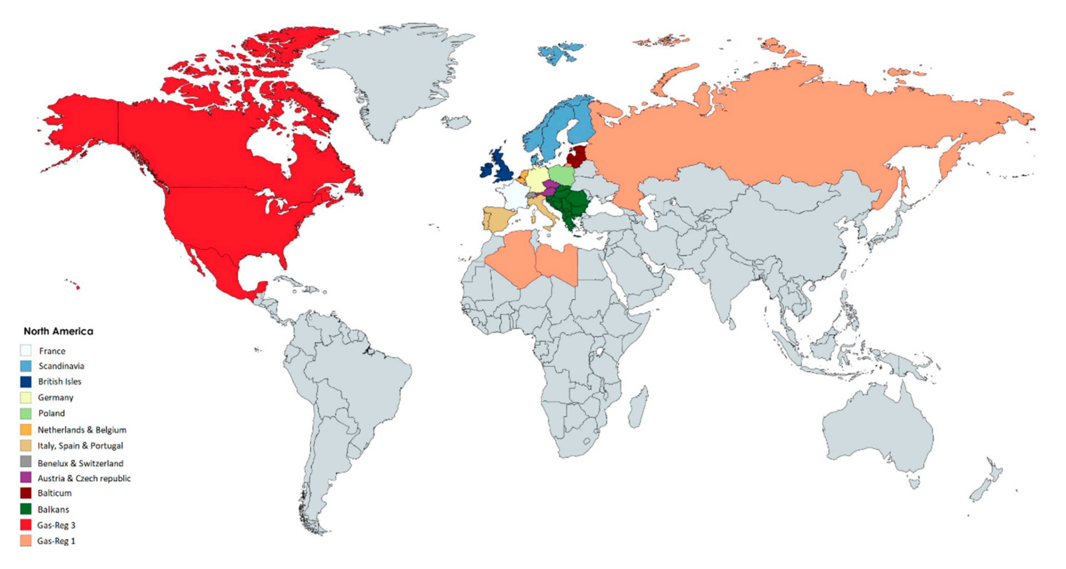
3.1. Spatial Resolution

In the natural gas sector, we consider intercontinental markets as Europe is highly dependent on imports. To tackle computational difficulties, we combine countries by building three regions, as illustrated in Figure 3. Region 1 represents dominant natural gas exporters including Russia, Algeria, and Libya. This region has no natural gas market but can export natural gas to the other two regions. In addition, it is the only region, which can practice market power. We consider North America as Region 2, which has both producers and a natural gas market. Europe is represented by Region 3, which has little production and depends on imports. We argue that the natural gas price spread between different countries in Europe is small. Thus, assuming a single gas price all of Europe as simplification is an expendable assumption.
The electricity markets are modelled only in Region 3 and consist of 11 market regions. Similar to the previous procedure, we merge neighboring countries and markets. In detail, these regions are Germany and Luxemburg, France, Poland, Scandinavian countries, Netherlands and Belgium, Switzerland and Italy, Austria and the Czech Republic, Iberia, Baltic States, and one region consisting of all eastern European countries as well as the Balkans. Heating markets are thereby considered in the first seven regions, focusing on the heating energy distributed via district heating—gas used directly for heating in buildings is included in the residential (and also partly in the industrial) gas demand. Similar to the gas markets, we argue the power price spread between neighboring countries is small, thus combining neighboring countries to avoid computational difficulties is adequate.

3.2. Temporal Resolution and Timeline

To consider the seasonal fluctuation of the natural gas demand, in each simulation year, the model includes three representative days in three different seasons: peak (winter), off-peak (summer), and the transition period between both seasons.
In the electricity market, instead of calculating the entire time horizon, we cluster hours with a similar residual load. This method has been used previously in many models for long-term generation capacity investment [28,29,30]. We choose residual load, as it contains the uncertainties of load and RES-E feed-in simultaneously [31]. We assume an average RES level of 65% when constructing the residual load to consider the effect of changing RES infeed with endogenous investments. We divide a year into three seasons representing winter, summer, and a transition season in between. We then cluster days with similar residual loads to four typical days in each season. To maintain a daily variation structure of the residual load, we divide these typical days into seven time segments, with shorter periods during the day and more extended periods during the night. Nahmmacher et al. [30] argued that 48 time slices (i.e., six representative days) are sufficient to obtain model results that are very similar to those obtained with a much higher temporal resolution. In the present work, we have built in total 84 time slices. The duration curve of real levelized residual load and constructed levelized residual load are shown in Figure 4.
The combined model runs in five-years intervals. We initially calibrate the system to the conditions of the year 2015 and subsequently simulate the years 2020, 2025, 2030, 2040 and 2050 as the timeline of the study.

3.3. Scenarios and Data Assumption

We consider four scenarios in this study. The scenario Comp assumes perfect competition in the gas markets. Our real case scenario is the Strategic Behavior scenario, which assumes a strategic behavior in the gas market. The scenario Strategic Behavior No Heat is similar to Strategic Behavior with the difference that it excludes the heating markets. The scenario High Market Power is also identical to the Strategic Behavior scenario, but it assumes higher market power in the gas sector. We use the data for the natural gas market presented in [24]. As discussed earlier, we use the approach of conjectural variations to define the market power. The mark-up factors are list in Appendix A. For the electricity and heating sector, we collected the data mainly from various public sources. Electrical capacities, exogenous investments and decommissioning of plants, and NTCs, are in line with [32]. For the heat demand time series as well as the thermal capacity of plants, we use the data and approach in [33]. The developments of fuel prices except for gas are in line with future prices in mid-term and with [34] in the long-term. The main characteristics of power plants, such as efficiencies, thermodynamic parameters, investment costs, etc., are listed in Table 1. These data are collected from various sources. For the calibration process, we backtested the model against the data of the year 2015 for the Strategic Behavior scenario since it is the scenario which is closer to the reality. In the backtesting process, we calibrate the emissions so that the modeled CO2 price corresponds the historical CO2 price. For the scenario without modeling the heating market, we also calibrate the Strategic Behavior No Heat with the historical CO2 price (Appendix B).

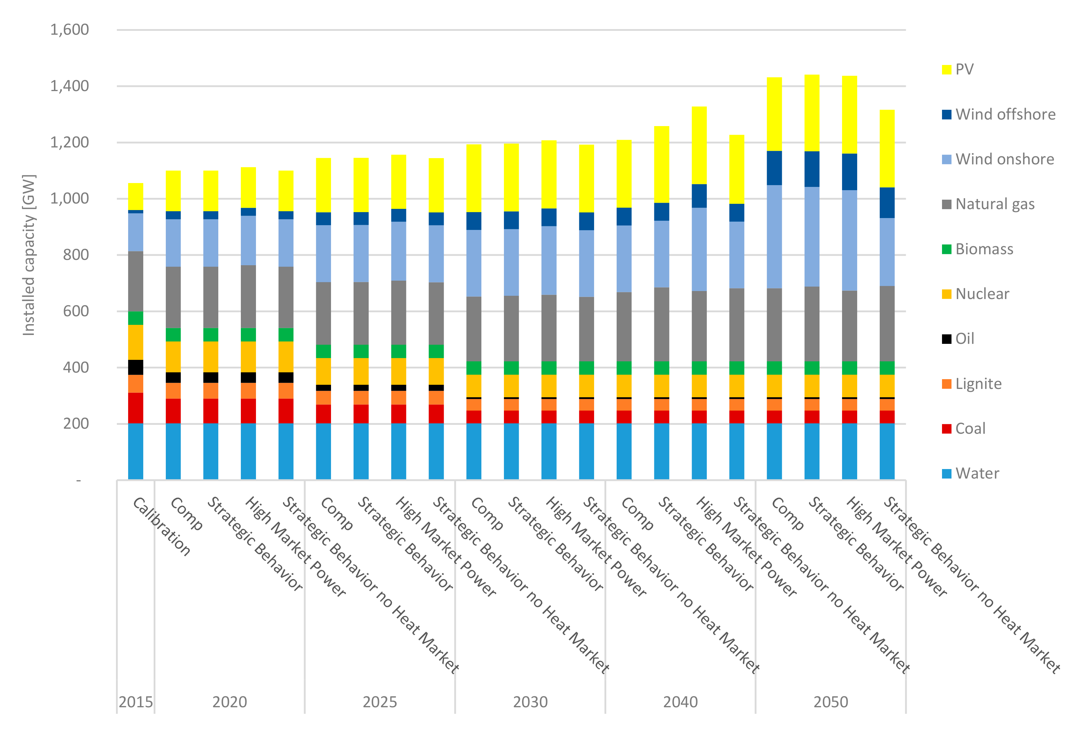
4. Results and Discussion

We describe the effect of strategic behavior in the natural gas sector in Section 4.1. As mentioned above, Strategic Behavior is the business as usual scenario. We compare the Strategic Behavior and Comp scenarios to discuss the effect of lower market power on the other sectors in Section 4.2. Similarly, we discuss the effect of higher market power on the other sectors by comparing the Strategic Behavior and High Market Power scenarios in Section 4.3. Section 4.4 discusses the impact and implications of modeling CHP units and the corresponding heat sector by comparing the Strategic Behavior and Strategic Behavior No Heat scenarios. In addition, we discuss the sensitivities of the results to various parameter variations in Appendix C.

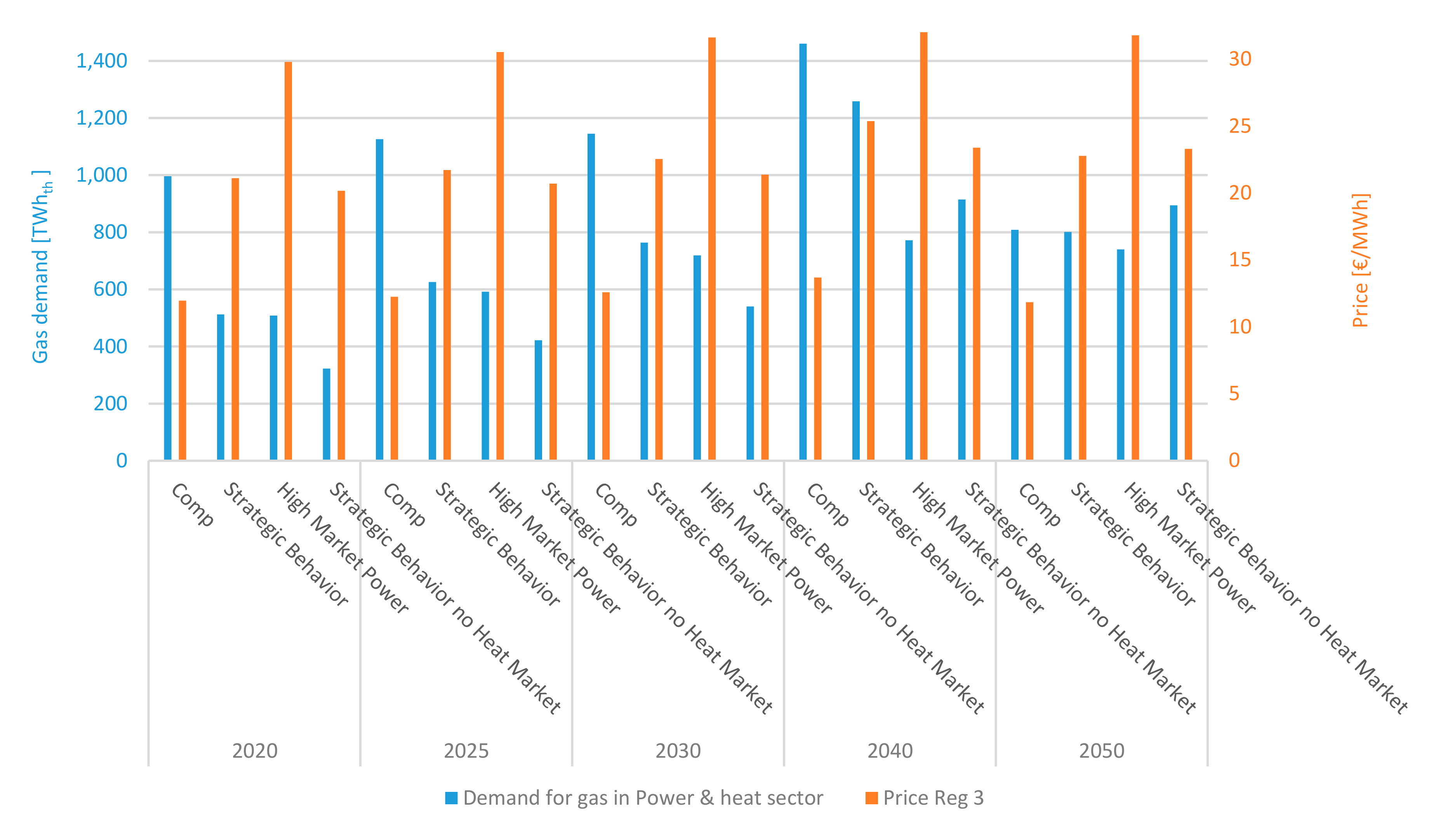
4.1. The Strategic Behavior in the Gas Market

Figure 5 shows the developments of gas prices and gas demand in the power sector for all the scenarios. As expected, the gas prices increase with the increase in mark-up factor and consequently the market power of gas exporters. The gas price is around 12 €/MWh for the Comp scenario, 22 €/MWh for the Strategic Behavior scenario, and 31 €/MWh for the High Market Power scenario in 2030. Different gas prices come also along with different demands for gas in the power sector as illustrated. Notably, the demand in the power sector is profoundly affected by the gas price increase. In 2020, the consumption of natural gas in the power sector is approximately 1000 TWhth in the Comp scenario, 517 TWhth in the Strategic Behavior scenario, and 500 TWhth in the High Market Power scenario. We conclude, after passing the current level of market power, any further increase in the gas prices by the exporters does not change the short-term gas consumption in the power and heat sectors since the 500 TWhth of gas demand is essential to meet the European demand for electricity and heat. From this amount, 47% is consumed in the CHP plants to meet the heat demand. We also see a decrease in the gas demand of the residential and industrial sectors with increasing market power. As mentioned above, we model these sectors using an inverse demand function. Besides, we observe that the peak of gas consumption in the power and heat sectors is in 2040 with a decrease afterward.

4.2. The Effect of Lower Market Power by Gas Exporters

Figure 6 shows the developments of the total power generation capacity in the entire region. By 2050, the total installed capacity for wind and PV is 750 GW for Comp scenario, 753 GW for Strategic Behavior scenario, and 764 GW for High Market Power scenario. Therefore, as a general observation, with increasing market power and gas prices, renewable investments increase slightly. Until 2050, the change in gas prices is affecting electricity generation, as illustrated in Figure 7.
In the Comp scenario, gas technologies become more competitive compared to coal and lignite and consequently the cheaper gas prices increase gas-fired electricity production. For example, in 2020, gas-fired electricity production is 440 TWhel. in the Comp scenario and 231 TWhel. in the Strategic Behavior scenario. In addition, until 2050, we observe lower CO2 prices in the Comp scenario compared to Strategic Behavior scenario, as shown in Table 2. This is explainable by the improved competitiveness of gas-fired generation compared to hard coal and lignite in the Comp scenario. This results in higher gas-fired electricity production (cf. Figure 7), which leads to a decrease in the demand for CO2 certificates.
The combination of cheap CO2 price and natural gas also reflects itself in the electricity prices. As illustrated in Figure 8, the electricity prices are higher in the Strategic Behavior scenario compared to the Comp scenario before 2050; e.g., in 2030, the average electricity price is 25 €/MWh in the Comp scenario and 45 €/MWh in the Strategic Behavior scenario.
In 2050, the situation changes though. In all the scenarios in this year, the emission cap limits even the full load hours of gas power plants. Although endogenous investments in renewables also occur in previous years, yet the significant part of these investments is made in this year. These investments are necessary to meet the electricity demand (cf. Figure 7). For these investments to be profitable, the electricity prices need to raise. This happens through an increase in the CO2 prices, since gas prices as other driver of power prices are rather driven by the profit maximization of the gas exporters and tend to decrease when tight CO2 bounds limit the usage of natural gas. The gas technologies bidding with their operational costs, set electricity prices in many time periods of the year even in 2050. Yet, their operating costs are higher in the Strategic Behavior scenario compared to the Comp scenario because of higher gas prices. Thus, in the Comp scenario, the CO2 prices rise to increase the electricity prices so that the electricity prices in the Comp and Strategic Behavior scenario are very close to approximately 66 €/MWh. Also, the system invests into PtH in 2050 to provide a part of heat demand using excessive renewable in-feed to meet the heat demand (Cf. Figure 9).

4.3. The Effect of Higher Market Power by Gas Exporters

Almost similar patterns are observable when comparing the Strategic Behavior and High Market Power scenarios. Until 2050, the higher gas prices in the High Market Power scenario lead to lower gas-fired electricity production (cf. Figure 7).
In 2020, other emission intensive technologies become competitive to gas plants in the High Market Power scenario and as a result the demand for CO2 certificates increase, which result in higher CO2 price. The combination of higher CO2 prices and higher operating costs of gas plants lead to higher electricity prices in the High Market Power scenario. These higher prices also make new investments profitable; accordingly, we observe 6.8 GW new investments in wind onshore and 5.3 GW in gas plants in 2020 (High Market Power is the only scenario with endogenous investments in 2020). The additional emission-free electricity from wind as well as the new efficient gas plants reduces the demand for emission certificates in the next simulation years until 2040 and, consequently, the CO2 price decreases. In addition, additional renewable production has a dampening effect on electricity prices in 2025 and 2030. In 2040, once again similar situations to 2020 happen.
In 2050, the heat and electricity generation of gas power plants reach the emission cap. The system hence makes considerable renewable investments, which require high electricity prices for repayment. As the gas prices are higher in the High Market Power scenario than in the Strategic Behavior scenario, a lower rise in the CO2 prices is required.

4.4. The Effect of Modelling Heating Market

As mentioned earlier, we also calibrate the Strategic Behavior No Heat with the historical CO2 price and therefore the total emission is higher (cf. Figure A1 in Appendix B). Comparing the Strategic Behavior and Strategic Behavior No Heat scenarios shows the impact of modeling the heating market alongside the electricity market. In 2020, we observe that the gas consumption is 517 TWhth in the Strategic Behavior scenario compared to 323 TWhth in the Strategic Behavior No Heat scenario (cf. Figure 5), due to must-run constraints for gas CHP generators and different total energy demand in these scenarios. The higher gas consumption in the Strategic Behavior scenario continues until 2050. In this period, we can also observe higher electricity prices (cf. Figure 8) in the Strategic Behavior scenario as a result of the operation of more expensive units to provide heat. Comparing the CO2 prices between Strategic Behavior No Heat and Strategic Behavior scenarios is very challenging as the total energy consumption and emission are different. In addition, in the Strategic Behavior No Heat scenario, fossil fuel technologies do not provide heat as in the Strategic Behavior scenario (cf. Table 2).
A reverse effect is observable in terms of gas consumption in 2050. On the one hand, the gas power plants need to meet the heating and electricity demand in the Strategic Behavior scenario. On the other hand, their full loads hours are limited due to emission constraints. This year, the system invests in renewable and PtH to meet the emission cap and demand for electricity and heat at the same time in the Strategic Behavior scenario. This additional investment increases the CO2 prices and consequently electricity prices, which lead to a different pattern of investments throughout the region. Therefore, we observe more renewable investments in the Strategic Behavior scenario and more investments in gas power plants in the Strategic Behavior No Heat scenario.

5. Conclusions

In the present paper, we develop a large-scale partial model based on the principles of Cournot–Nash equilibria, which includes the sectors of natural gas, electricity and heating as well as emission trading. We model four different scenarios to analyze the effect of strategic behavior in the natural gas sector and study the impact of modeling the heating sector coupled with the power sector.
We observe that, as the market power in the gas sector increases, gas becomes more expensive. The gas price in the scenario with the highest market power is 2.6times higher than in the scenario without no strategic behavior. Besides, a minimum of 500 TWhth of gas consumption is required to meet the European power and heat demands in the short run. We conclude that this demand will not be affected dramatically by practicing higher market power. However, lower market power can have a considerable effect on the short-term gas consumption in the power sector.
The results of the paper also support that more pronounced strategic behavior leads to higher renewable investments in the power sector and higher PtH’s investments in the heating sector. At the same time, long-term gas CHP and boiler investments decrease with increasing strategic behavior.
We also observe that weaker strategic behavior results in lower electricity prices before 2050 because of the reduction in operating costs of gas power plants. Consequently, gas-fired power generation substitutes more easily coal-fired generation, leading to a reduction in the demand for CO2 certificates. Therefore, we conclude that lower market power leads to lower CO2 prices before 2050. We observe the opposite phenomenon in the scenario with high market power. As the strategic behavior and consequently gas prices increase, other thermal technologies such as coal and lignite become competitive to gas. Since these technologies are more carbon intensive, the demand for CO2 certificate increases. In addition, the combination of higher gas and CO2 prices increases the power prices and fosters renewable investments.
In 2050, however, as fossil fuels play only a minor role in the power and heating sector and coal is completely driven out of the market, the change in the strategic behavior of gas exporters has a minor effect on electricity prices, as the number of hours where gas is setting the prices are limited. At the same time, the system needs to invest in renewables to provide electric energy while meeting the emission boundary. Therefore the CO2 prices increase in the scenario with lower gas prices (i.e., competitive gas markets) to sustain a certain level of power prices, ensuring the profitability of renewable investments. Thus, we conclude that less strategic behavior leads to higher CO2 prices in 2050.
We also identify the benefits of modeling the district heating sector jointly with the electricity sector and deliver a mixed complementarity formulation for the combined power and heating sector as one of the few available academic sources. Dispatch and commitment models generally underestimate gas-fired generation for many reasons (e.g., the lack of enough price scarcity). Modeling the heating sector, along with the power sector, can boost gas consumption because of the must-run conditions of gas-fired CHPs. Higher gas consumption in the power sector will affect power prices, investments, etc.
System operators as well as regulators and economists can use the approach presented in this paper. The present approach can be expanded by using detailed demand data instead of load segments in the future works, to provide outcomes that are more precise.

Funding

This research was funded by Federal Ministry of Economic Affairs and Energy, through the project “LKD-EU”, grant number 03ET4028D.

Acknowledgments

The author thanks Christoph Weber for his constructive comments.

Conflicts of Interest

The authors declare no conflict of interest.

Nomenclature

Superscripts and indices:
E Electricity d Demand for electricity
H Heat E Emission cap
G Gas L Capacity
P Producer D Duration of time segments
C Consumer η Efficiency
f Index gas region F Fuel cost
n ,   n Index electricity region C V Electricity reduction factor
z Index technology class C B Power-to-heat ratio
l Index load segment ρ Availability
t Index season η S l o p e Efficiency slope within technology groups
g Index gas sector ε Price elasticity
Q Grid transmission β Emission intensity
e x t . Extraction turbine E Emission cap
b k p . Backpressure turbineVariables
r e s . Electricity production technologies excluding backpressure q Production
c o n d . Condensing turbine λ Price
t h Thermal u Electricity consumption of pumps
e Electric L n e w Investment in new capacity
t o t Total ϑ Shadow price for capacity
b Index fuel τ Dual variable
P t H Power-to-Heat
P t G Power-to-Gas
O H Only heat
CCGTCombined cycle gas turbine
GTGas turbine
STSteam turbine
Parameters:
A n n Annualized investment cost

Appendix A. Parameters for Modelling Strategic Behaviour

Table A1. Mark-up factors for gas regions. 0 means no market power and 1 means that the trader is a full Cournot player.
CompStrategic BehaviorHigh Market PowerStrategic Behavior no Heat
Reg 100.10.250.1
Reg 200.10.250.1
Reg 30000

Appendix B. CO2 Emission Cap

Figure A1. Developments of emission cap for the electricity market.
Energies 13 05040 g0a1

Appendix C. Sensitivity Considerations

It is a common approach among similar studies to model possible future situations through the scenario technique. As discussed earlier, the present study aims to investigate the effect of the strategic behavior of the gas suppliers on the power, heating and emission trading rather than depicting a precise possible future pathway. Thus, we avoided considering many long-term uncertain factors.
However, from our perspective, factors such as political uncertainty (e.g., change in market design, the possibility of an economic depression, international dispute, etc.), technology developments, demand developments, change in fuel prices are relevant. Among these uncertain factors, we believe political uncertainties require further investigations caused by the broadness and complexity of the subject. We have not modeled the uncertainties in the coal, oil and lignite prices since these commodities’ roles will be weaker and weaker in the future. Besides, using a similar approach, we observe that their effect is minor [34].
The uncertainties in demand development are mainly caused by increasing the level of electrification in heating transportation and GDP growth. We already model the electrification in the heating sector by introducing the investment in PtH, yet avoid considering the transportation sector and the GDP growth. We believe the effect of GDP growth is negligible, while the transportation sector can add approx. 7% to the electrical demand according to our calculations (this number is rather similar to the estimate given in [35]). We anticipate that considering this demand growth will result in higher renewable investment and higher CO2 prices in all the scenarios, as increasing the CO2 price is the main path to trigger more renewable investments in the model. is a common approach among similar studies to model possible future situations through the scenario technique. As discussed above, the present paper aims to investigate the effect of the strategic behavior of the gas suppliers on power, heating, and emission trading rather than depicting a precise possible future pathway. Thus, we avoid considering many long-term uncertain factors.
However, from our perspective, factors such as political uncertainty (e.g., change in market design, the possibility of an economic depression, international dispute, etc.), technology developments, demand developments, and change in fuel prices are relevant. Among these uncertain factors, we believe political uncertainties require further investigations due to the broadness and complexity of the subject. We do not model the uncertainties in the coal, oil, and lignite prices since these commodities’ roles will be weaker and weaker in the future. Besides, using a similar approach, we observe that their effect is minor [35].
The uncertainties in demand development are mainly caused by increasing the level of electrification in heating transportation and GDP growth. We model the electrification in the heating sector by introducing the investment in PtH but avoid considering the transportation sector and the GDP growth. We believe the effect of GDP growth is negligible, while the transportation sector can add approximately 7% to the electrical demand according to our calculations (this number is very close to those of similar scenarios [36]). We believe that considering this demand growth can result in higher renewable investment and higher CO2 prices in all scenarios, as increasing the CO2 price is the only way to trigger more investments in the model.

References

  1. European Commission Oil, Gas and Coal. Available online: https://ec.europa.eu/energy/en/topics/oil-gas-and-coal (accessed on 19 May 2019).
  2. Statistical Review of World Energy, Energy Economics, Home. Available online: https://www.bp.com/en/global/corporate/energy-economics/statistical-review-of-world-energy.html (accessed on 26 July 2020).
  3. “Washington Post,” Washington Post. Available online: https://www.washingtonpost.com/gdpr-consent/ (accessed on 26 July 2020).
  4. European Commission Secure Gas Supplies. Available online: https://ec.europa.eu/energy/topics/energy-security/secure-gas-supplies_en (accessed on 26 July 2020).
  5. Jimenez-Navarro, J.-P.; Kavvadias, K.; Filippidou, F.; Pavičević, M.; Quoilin, S. Coupling the heating and power sectors: The role of centralised combined heat and power plants and district heat in a European decarbonised power system. Appl. Energy 2020, 270, 115134. [Google Scholar] [CrossRef]
  6. Roach, M.; Meeus, L. The welfare and price effects of sector coupling with power-to-gas. Energy Econ. 2020, 86, 104708. [Google Scholar] [CrossRef]
  7. Emonts, B.; Reuß, M.; Stenzel, P.; Welder, L.; Knicker, F.; Grube, T.; Görner, K.; Robinius, M.; Stolten, D. Flexible sector coupling with hydrogen: A climate-friendly fuel supply for road transport. Int. J. Hydrogen Energy 2019, 44, 12918–12930. [Google Scholar] [CrossRef]
  8. Pavičević, M.; Mangipinto, A.; Nijs, W.; Lombardi, F.; Kavvadias, K.; Jiménez Navarro, J.P.; Colombo, E.; Quoilin, S. The potential of sector coupling in future European energy systems: Soft linking between the Dispa-SET and JRC-EU-TIMES models. Appl. Energy 2020, 267, 115100. [Google Scholar] [CrossRef]
  9. Brown, T.; Schlachtberger, D.; Kies, A.; Schramm, S.; Greiner, M. Synergies of sector coupling and transmission reinforcement in a cost-optimised, highly renewable European energy system. Energy 2018, 160, 720–739. [Google Scholar] [CrossRef] [Green Version]
  10. Steinmann, W.-D.; Bauer, D.; Jockenhöfer, H.; Johnson, M. Pumped thermal energy storage (PTES) as smart sector-coupling technology for heat and electricity. Energy 2019, 183, 185–190. [Google Scholar] [CrossRef]
  11. Möst, D.; Perlwitz, H. Prospects of gas supply until 2020 in Europe and its relevance for the power sector in the context of emission trading. Energy 2009, 34, 1510–1522. [Google Scholar] [CrossRef]
  12. Erdener, B.C.; Pambour, K.A.; Lavin, R.B.; Dengiz, B. An integrated simulation model for analysing electricity and gas systems. Int. J. Electr. Power Energy Syst. 2014, 61, 410–420. [Google Scholar] [CrossRef]
  13. He, C.; Liu, T.; Wu, L.; Shahidehpour, M. Robust coordination of interdependent electricity and natural gas systems in day-ahead scheduling for facilitating volatile renewable generations via power-to-gas technology. J. Mod. Power Syst. Clean Energy 2017, 5, 375–388. [Google Scholar] [CrossRef] [Green Version]
  14. Deane, J.P.; Ciaráin, M.Ó.; Gallachóir, B.P.Ó. An integrated gas and electricity model of the EU energy system to examine supply interruptions. Appl. Energy 2017, 193, 479–490. [Google Scholar] [CrossRef]
  15. Hauser, P.; Heidari, S.; Möst, D.; Weber, C. Does Increasing Natural Gas Demand in the Power Sector Pose a Threat of Congestion to the German Gas Grid? A Model-Coupling Approach. Energies 2019, 12, 2159. [Google Scholar] [CrossRef] [Green Version]
  16. Gabriel, S.A.; Conejo, A.J.; Fuller, J.D.; Hobbs, B.F.; Ruiz, C. Complementarity Modeling in Energy Markets; 6161; Springer: New York, NY, USA, 2013; Volume 180, ISBN 978-1-4419-6122-8. [Google Scholar]
  17. Ruiz, C.; Conejo, A.J.; Fuller, J.D.; Gabriel, S.A.; Hobbs, B.F. A tutorial review of complementarity models for decision-making in energy markets. EURO J. Decis. Process. 2014, 2, 91–120. [Google Scholar] [CrossRef] [Green Version]
  18. Gabriel, S.A.; Kiet, S.; Zhuang, J. A Mixed Complementarity-Based Equilibrium Model of Natural Gas Markets. Oper. Res. 2005, 53, 799–818. [Google Scholar] [CrossRef]
  19. Egging, R.; Gabriel, S.A.; Holz, F.; Zhuang, J. A complementarity model for the European natural gas market. Energy Policy 2008, 36, 2385–2414. [Google Scholar] [CrossRef] [Green Version]
  20. Spiecker, S. Modeling Market Power by Natural Gas Producers and Its Impact on the Power System. IEEE Trans. Power Syst. 2013, 28, 3737–3746. [Google Scholar] [CrossRef]
  21. Abrell, J.; Weigt, H. The Short and Long Term Impact of Europe’s Natural Gas Market on Electricity Markets until 2050. Energy J. 2016, 37. [Google Scholar] [CrossRef]
  22. Virasjoki, V.; Siddiqui, A.S.; Zakeri, B.; Salo, A. Market Power With Combined Heat and Power Production in the Nordic Energy System. IEEE Trans. Power Syst. 2018, 33, 5263–5275. [Google Scholar] [CrossRef] [Green Version]
  23. Spiecker, S. Analyzing Market Power in a Multistage and Multiarea Electricity and Natural Gas System. In Proceedings of the 8th International Conference on the European Energy Market (EEM), Zagreb, Croatia, 25–27 May 2011. [Google Scholar]
  24. Heidari, S.; Weber, C. The changing landscape of world gas markets at the horizon 2020. In Proceedings of the 14th International Conference on the European Energy Market (EEM), Dresden, Germany, 6–9 June 2017; pp. 1–6. [Google Scholar]
  25. Barth, R.; Brand, H.; Meibom, P.; Weber, C. A Stochastic Unit-commitment Model for the Evaluation of the Impacts of Integration of Large Amounts of Intermittent Wind Power. In Proceedings of the International Conference on Probabilistic Methods Applied to Power Systems, PMAPS 2006, Stockholm, Sweden, 11–15 June 2006; pp. 1–8. [Google Scholar]
  26. Kunz, F. DIW Berlin: Electricity, Heat and Gas Sector Data for Modelling the German System. DIW Berlin. 2017. Available online: http://www.diw.de/sixcms/detail.php?id=diw_01.c.574115.de (accessed on 10 January 2018).
  27. Weber, C. Uncertainty in the Electric Power Industry: Methods and Models for Decision Support; International Series in Operations Research & Management Science; Springer: New York, NY, USA, 2005; ISBN 978-0-387-23047-4. [Google Scholar]
  28. Spiecker, S.; Weber, C. The future of the European electricity system and the impact of fluctuating renewable energy—A scenario analysis. Energy Policy 2014, 65, 185–197. [Google Scholar] [CrossRef]
  29. Gerbaulet, C.; Lorenz, C. dynELMOD: A Dynamic Investment and Dispatch Model for the Future European Electricity Market. DIW Berlin. 2017. Available online: https://www.diw.de/sixcms/detail.php?id=diw_01.c.558131.de (accessed on 23 May 2018).
  30. Nahmmacher, P.; Schmid, E.; Hirth, L.; Knopf, B. Carpe diem: A novel approach to select representative days for long-term power system modeling. Energy 2016, 112, 430–442. [Google Scholar] [CrossRef]
  31. De Sisternes Jimenez, F.; Webster, M.D. Optimal Selection of Sample Weeks for Approximating the Net Load in Generation Planning Problems. Massachusetts Institute of Technology. Engineering Systems Division, Working Paper. January 2013. Available online: http://dspace.mit.edu/handle/1721.1/102959 (accessed on 23 May 2018).
  32. ENTSO-E. Ten-Year Network Development Plan 2018. 2018. Available online: https://tyndp.entsoe.eu/tyndp2018/ (accessed on 6 February 2019).
  33. Kunz, F.; Weibezahn, J.; Hauser, P.; Heidari, S.; Schill, W.-P.; Felten, B.; Kendziorski, M.; Zech, M.; Zepter, J.; Von Hirschhausen, C.; et al. Electricity, Heat, and Gas. Sector Data for Modeling the German System; Schriften des Lehrstuhls für Energiewirtschaft; TU Dresden: Dresden, Germany, 2018. [Google Scholar]
  34. IEA. World Energy Outlook 2019—Analysis. Available online: https://www.iea.org/reports/world-energy-outlook-2019 (accessed on 5 December 2019).
  35. Heidari, S.; Weber, C. The role of Power-to-Gas in the future energy systems; A case study for Germany and selected neighboring countries. In Proceedings of the 7th International Ruhr Energy Conference, Essen, Germany, 24 September 2018. [Google Scholar]
  36. European Environment Agency Electric Vehicles and the Energy Sector—Impacts on Europe’s Future Emissions. Available online: https://www.eea.europa.eu/publications/electric-vehicles-and-the-energy/download#:~:text=The%20share%20of%20electricity%20consumption,vehicles%20anticipated%20in%20each%20country (accessed on 19 May 2019).
Figure 1. Structure of CElGEM-Model.
Energies 13 05040 g001
Figure 2. Simplified Power-Heat diagram for backpressure (right) and extraction (left) units [26].
Energies 13 05040 g002
Figure 3. Spatial resolution of the CElGEM-Model.
Energies 13 05040 g003
Figure 4. Levelized duration curve of residual load for the considered electricity markets with 65% renewables share.
Energies 13 05040 g004
Figure 5. Developments of natural gas demand and gas price.
Energies 13 05040 g005
Figure 6. Developments of the endogenous and exogenous electrical capacity.
Energies 13 05040 g006
Figure 7. Electricity production mix for the entire region.
Energies 13 05040 g007
Figure 8. Developments of electricity prices for selected regions.
Energies 13 05040 g008
Figure 9. Developments of the installed heating capacity of CHP units and other heat sources by fuel.
Energies 13 05040 g009
Table 1. Characteristics of new and existing generation technologies.
Cost Misc.Elec EfficiencyTot. EfficiencyCBCVInvestment Costs
New[€/MWh][%][%] [€/kW]
CCGT bkp.1.644%82%1.10 1170
CCGT ext.1.659%82%1.100.171170
CCGT cond.1.659% 900
GT1.640% 450
sun-100% From [29]
wind off-100% From [29]
wind on-100% From [29]
Existing
CCGT bkp.3.9843%82%1.12
CCGT ext.3.9853%82%1.110.17
CCGT cond.3.9854%
gas ST bkp.4.2825%82%0.43
gas ST ext.4.2835%82%0.460.15
gas ST cond.4.2837%
GT4.2246%
nuclear0.5233%
biomass bkp.1.5021%70%0.43
biomass ext.1.5028%70%0.240.15
biomass cond.1.5030%
coal bkp.2.2426%85%0.43
coal ext.2.2434%85%0.460.15
coal cond.2.2436%
lignite bkp.1.6522%85%0.35
lignite ext.1.6532%85%0.420.15
lignite cond.1.6533%
Table 2. Developments of CO2 prices.
CompStrategic BehaviorHigh Market PowerStrategic Behavior No Heat
2020112435
2025115135
2030120135
204027505934
205021717212776

