Abstract
Power distribution systems nowadays are highly penetrated by renewable energy sources, and this explains the dominant role of power electronic converters in their operation. However, the presence of multiple power electronic conversion units gives rise to the so-called phenomenon of Constant Power Loads (CPLs), which poses a serious stability challenge in the overall operation of a DC micro-grid. This article addresses the problem of enhancing the stability margin of boost and buck-boost DC-DC converters employed in DC micro-grids under uncertain mixed load conditions. This is done with a recently proposed methodology that relies on a two-degree-of-freedom (2-DOF) controller, comprised by a voltage-mode Proportional Integral Derivative (PID) (Type-III) primary controller and a reference governor (RG) secondary controller. This complementary scheme adjusts the imposed voltage reference dynamically and is designed in an optimal fashion via the Model Predictive Control (MPC) methodology based on a specialized composite (current and power) estimator. The outcome is a robust linear MPC controller in an explicit form that is shown to possess interesting robustness properties in a wide operating range and under various disturbances and mixed load conditions. The robustness and performance of the proposed controller/observer pair under steady-state, line, and mixed load variations is validated through extensive Matlab/Simulink simulations.
1. Introduction
Modern DC micro-grids are preferred over conventional AC power grids, as they are better suited to the integration of energy storage devices together with renewable and alternative power sources, due to their inherent DC character. Other popular equipment, such as computers and servers in data centers, or even plug-in hybrid vehicles are also of a DC nature in the form of electronic loads. However, the integration of sources, loads, as well as energy storage devices requires the use of several different voltage levels, offered by multiple power electronic conversion units acting as interfaces between subsystems with different voltages. These architectures are not free of stability issues because they act as Constant Power Loads (CPLs), which exhibit a negative impedance behavior, unlike with typical resistive loads (constant voltage loads, i.e., CVLs). CPLs are observed in the cascade connection of DC-DC converters, e.g., in the case of motor drives or electronic loads, where there exists a downstream converter whose operation is tightly regulated by closed-loop control to maintain a desired output voltage. In such cases, the power absorbed by the load will be constant, i.e., when the output voltage drops in the face of a disturbance the current will be increased. This phenomenon introduces nonlinearity and can potentially result in instability (unlimited current) if not properly dealt with. Further details and a thorough understanding of these issues can be found in References [1,2,3].
Recent years have witnessed increased interest in the control of all types of DC-DC converters. Many advanced control methods have been recently proposed with the aim of improving their transient response and robustness [4,5,6,7,8,9,10,11,12,13]. Optimal and nonlinear system approaches using LQR, Linear Matrix Inequalities (LMIs) convex optimization, or parameter-dependent Lyapunov functions and corresponding time-varying parameter-dependent (gain-scheduled) control laws have been studied in References [4,5,6]. A set-theoretic approach to the constrained stabilization of power converters on the basis of bilinear dynamics using piecewise-linear Lyapunov functions has been introduced in Reference [7] and several hybrid control methods have been tested in Reference [8]. The Model Predictive Control (MPC) technology has also been extensively applied to the voltage regulation problem of DC-DC converters in an implicit or explicit form [9,10,11,12,13]. More recently, a number of papers have considered the robust control of converters in DC Micro-grids. In Reference [14], the authors adopt a polytopic uncertainty model and convex optimization for islanded DC micro-grids under plug-and-play (PnP) functionality of distributed generations (DGs). In References [15,16], the authors deal with the robust voltage control problem of boost converters with nonlinear control methodologies, such as sliding mode [15] and passivity-based [16] control.
Unfortunately, all these studies have considered only the trivial case of resistive loads, i.e., CVLs. More recent studies have proposed nonlinear control designs for addressing the CPL issue on a large-signal basis, see e.g., [17,18,19,20] and references therein. In Reference [17], a passivity-based controller for a buck-boost converter is proposed that relies on a CPL power estimator for performance improvement. It is shown that these converter types have bilinear second-order dynamics which, in the presence of CPLs, become non-minimum phase with respect to both states. In References [18,19], solutions using sliding mode control are proposed, whereas Reference [20] presents an MPC solution for a boost converter in DC Micro-grids.
In this work, we follow the most realistic approach, i.e., we consider situations with mixed load conditions where uncertain CPLs and CVLs are combined. Moreover, we also consider situations in which the main controller is already hardcoded or implemented in low-cost hardware that we would not like or it is not possible to replace. Instead of replacing this controller, a new idea is to complement it with a secondary higher-level controller that provides a dynamically modified reference signal to the primal controller. This idea results in a two-degrees-of-freedom (2-DOF) control structure where the secondary controller can also run at a different (slower) rate. Such schemes are the so-called reference governors (RGs), which have only very recently appeared in the power electronics field [21,22,23,24,25]. The underpinning theory has been developed for over two decades and applied already to other engineering fields, mainly in the automotive industry and robotics, see, e.g., [26,27,28] and references therein.
DC-DC boost and buck-boost converters are increasingly preferred in power distribution systems for their flexibility since they can step up or down the voltage between the source and the load. In the case of classical resistive loads, which behave as passive impedances, their control is standard and mature. This is not the case in modern applications with CPLs, which pose new challenges to control design. Our recent work in Reference [22] has considered a buck-boost converter and applied the 2-DOF idea with a Proportional Integral Derivative (PID) Type-III primary controller and an RG designed optimally using MPC theory. This work has been developed for classical resistive loads (CVL) only. In the present article, for the first time in the literature, to the best of our knowledge, this framework is extended to cover the case of additional CPLs. The main results of this paper are equally well applied to the two most common boost-type DC-DC converters, i.e., boost and buck-boost. However, to avoid overloading of the paper, a decision was made to concentrate on the buck-boost case in the sequel.
This paper is structured as follows. Section 2 describes the DC-DC buck-boost converter in a new composite load (CVL + CPL) setting and Section 3 outlines the 2-DOF controller recently proposed in the literature, and the main motivation behind this research with an illustrative example. In Section 4, a new 2-DOF control and estimator design is proposed to deal with the CPL load case. The main numerical results that support the new methodology are included in Section 5. The final section concludes.
2. DC-DC Buck-Boost Converter Feeding a Composite Load
The circuit diagram of a buck-boost converter with a typical resistive load is shown in Figure 1. A non-ideal circuit with parasitic elements rL, rC of the inductor L and the capacitor C is adopted. As a basis for comparison purposes, in the sequel, all values and parameter ranges of the buck-boost converter used in this paper are taken from Reference [22] and are summarized in Table 1, where fs is the switching frequency of the Pulse Width Modulator (PWM) and D is the duty cycle taking values in the interval [0,1]. However, when such a converter is part of a DC micro-grid, a totally different type of loading is possible, i.e., the so-called Constant Power Load (CPL). This phenomenon cannot be disregarded in control designs by considering only common resistive loads (CVLs). The realistic approach is to consider situations with mixed load conditions, where uncertain CPLs and CVLs are combined, as shown in Figure 1, by adding an extra load path, designated as CPL. The CVL and CPL loads are denoted by R, RCPL respectively. In the sequel, an analysis considering a composite load (CVL + CPL) will be presented.
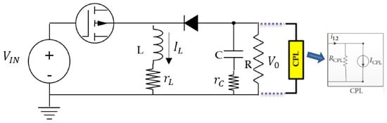
Figure 1.
Buck-boost converter circuit.

Table 1.
Buck-boost converter parameter values and ranges.
3. Review of the Hybrid Control Design Scheme and Main Motivation
In this section, we begin with an informal presentation of the main results of this paper, in terms of an example considered in a recent publication, which serves as a good starting point for conveying the main motivation of our work.
A standard control strategy in industrial applications, including power electronics, is the Proportional Integral Derivative (PID) controller. This controller is usually known as the Type-III compensator in power electronics and its design is usually performed based on the so-called small-signal model of the converter in the frequency domain [29]. Typical requirements are a phase margin (PM) above 45 deg and a gain margin (GM) over 10 dB. The transfer function of the PID Type III compensator in its most general form is:
This control strategy has been evaluated in Reference [22] in an application scenario from ([29], chapter 5, design 5.3.1). The design parameters for the PID type-III controller (3) proposed in Reference [22] are given below in Table 2.
Table 2.
Proportional integral derivative (PID) type-III specifications (rad/s).
As shown recently in References [21,22], further performance enhancement is possible using a hybrid scheme combining a PID and a predictive controller. The predictive controller is in digital form and has the role of a reference governor (RG) as explained pictorially in Figure 2. It is a secondary controller responsible for producing a dynamically modified optimal reference signal r(k) from a desired set-point signal rd(k). The MPC reference governor (MPC RG) uses a linear model of the closed-loop system (including the PID type-III controller) to predict future trajectories and make optimal decisions for r(k). This is done through the following static relation (for more details see the analysis in Section 4.2) in discrete-time where k is the current sampling instant:
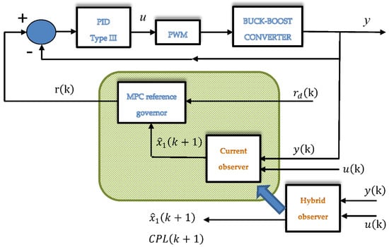
Figure 2.
Hybrid (combined PID Type-III and model predictive control (MPC) reference governor) control scheme for a buck-boost converter with an old (current only) and a new hybrid observer (current and constant power load (CPL) power).
For the buck-boost converter of Table 1, an MPC RG has been proposed in Reference [22] with gains Kr, Kx as in Table 3, which have been produced using the specs in Table 4. It is noteworthy that the optimal MPC RG takes an explicit static state-feedback form, where the gains of the controller are fixed and can be a priori determined.
Table 3.
MPC RG gains for rw = 50.
Table 4.
MPC reference governor (RG) specifications.
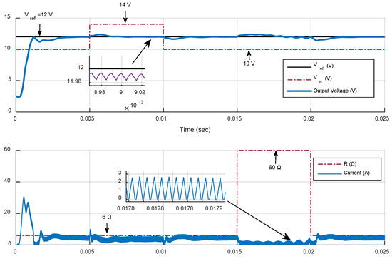
Figure 3 and Figure 4 reveal the performance improvements resulting from the addition of the MPC RG to a primal PID type-III controller in four different cases, i.e., (a) a startup transient in boost mode and light load conditions (R = 6 Ω), (b) line voltage step changes from 10 to 14 V (boost to buck) or 14 to 10 V (buck to boost), and (c) large load perturbations (from R = 6 Ω to R = 60 Ω) in boost mode. It is clear from all four different tests that the PID type-III controller alone suffers from long settling times due to highly oscillatory behavior, giving also rise to large current spikes in the initial phase of the transients and prolonged current saturation in many cases. It is also evident that the MPC RG scheme provides significant improvements in terms of rise time, settling time, and overcurrent avoidance. Further details can be found in Reference [22]. Similar conjectures are made in other publications with buck or boost converters and RG schemes [21,22,23,24,25].
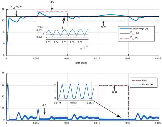
Figure 3.
Transient responses of the PID Type-III controller for varying Vin and resistive load R. Four cases are considered: Startup transient response for an input voltage Vin = 10 V (Boost mode) and R = 6 Ω; Input voltage step change from Vin = 10 V to 14 V (Boost to Buck mode) for R = 6 Ω; Input voltage step change from Vin = 14 V to 10 V (Buck to Boost mode) for R = 60 Ω; load step change (from 60 Ω to 6 Ω) in Boost mode (Vin = 10 V).
However, all these results in previous publications have only considered the case of a resistive load (CVL). What happens when such a converter is included in a DC micro-grid, where its operation will be affected by other converters, hence imposing an additional CPL loading. The negative impedance instabilities caused by CPLs are well known [1,2,3], hence a robust control scheme is necessary to deal with additional uncertain CPL loads. Especially when the ratio between the CPL and CVL load is much larger than unity, the imposed operating conditions are far from the nominal ones, in which the converter controller has been designed. Therefore, the main motivation of the work presented herein is to investigate whether:
- it is necessary to redesign the controller(s). This is important since the main controller may be already hardcoded or implemented in low-cost hardware, where redesign should be avoided for cost reasons or simply because it is not possible to be replaced.
- linear controllers and designs are adequate. If not, it might be necessary to resort to more complicated nonlinear control methodologies.
- minimal modifications of the initial design are sufficient to achieve acceptable performance and good robustness properties, in the presence of an unknown mixture of CPL and CVL, while avoiding the cost of adding extra sensors into the system.
To investigate further these issues, which are the main purpose of this work, we carried some Matlab simulation experiments. We used the same buck-boost converter control design discussed before in (3) and (4). To stress-test this design, we inject a varying CPL load in boost mode—which poses most difficulties—while keeping the CVL load and supply voltage constant. For a resistor value of , which corresponds to a CVL load , CPL loads with Pr much larger than unity are injected. For the PID type-III controller, the results are depicted in Figure 5. It is clear that significant ringing (oscillations) occurs as the amount of CPL load injected is progressively increased. Instability is detected when the ratio Pr becomes close to 3 or 4 (72 to 96 W).
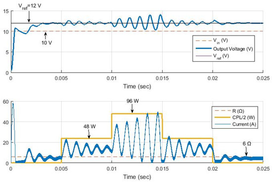
Figure 5.
Transient responses of the PID Type-III controller for constant Vin, R, and varying CPL load in boost mode. Significant ringing occurs as the amount of CPL load injected is progressively increased. Instability is detected when the ratio Pr becomes close to 3 or 4 (72 to 96 W).
The same mixed load conditions are then injected to the same converter, controlled with the combination of PID Type III controller and MPC RG. The new results with the addition of the reference governor are shown in Figure 6. We observe a totally different picture: the composite controller shows very good robustness properties for ratios Pr up to 4 (96 W). The robustness limits of this controller are further investigated using much larger ratios Pr of up to 10 (240 W) (It is noted that testing the converter with a power of 240 W, i.e., ten times the rated power, could not be performed in reality, as it gives rise to significantly high currents that would lead to inductor saturation. However, although not realistic, this extreme condition situation is tested in simulation to investigate the stability and robustness margins of the proposed control policy). The controller shows remarkable robustness properties as Figure 7 reveals. For larger CPL loads the controller fails, however, this test shows the significant robustness properties of the hybrid controller—which is a combination of simple linear controllers—that has been designed at a very different operating point and loading conditions.
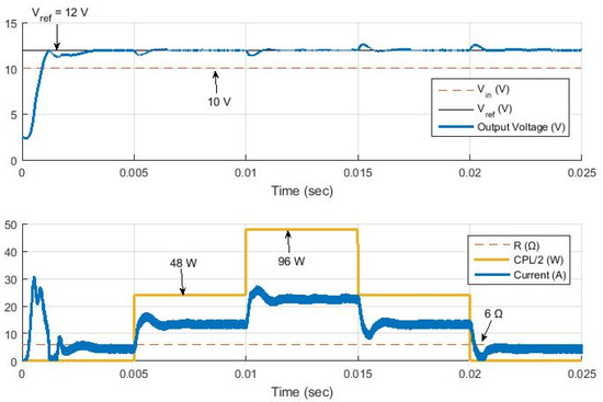
Figure 6.
Transient responses of the hybrid controller (PID Type-III + MPC RG) for constant Vin = 10 V, R = 6 Ω, and varying CPL load in boost mode, for ratios Pr up to 4 (96 W).
Figure 7.
Transient responses of the hybrid controller (PID Type III + MPC RG) for constant Vin = 10 V, R = 6 Ω, and varying CPL load in boost mode. The converter’s robustness limits are investigated with ratios Pr up to 10 (240 W).
It is worth noting that the robust results shown before were obtained without retuning any of the two controllers. However, the presence of the RG was critical, as the primary controller alone could not deal with CPLs. A key ingredient was the modification of the estimator feeding the RG. The estimator’s role is very important in order to avoid the addition of extra sensors, e.g., for the CPL power absorbed, which is difficult to measure in real situations. As shown in Figure 2, the key modification is the replacement of the current estimator used in previous designs by a new hybrid estimator, which provides robust estimates for both inductor current and CPL power. These issues are formally presented and discussed in the following sections.
4. A New Hybrid Control and Estimator Design for a Voltage-Mode Controlled Buck-Boost Converter
In this section, all details for the development of a new optimal and efficient hybrid control scheme (PID type-III + MPC RG) using the linear MPC methodology, in the presence of CPLs, are given. Although presented in detail in recent publications, the basic modeling steps and MPC optimization is briefly reviewed, for completeness. The main contribution is the development of a new hybrid observer, which is important for achieving a high and robust performance without the need for redesign or costly expansions with extra sensors.
An MPC-based design procedure is commonly performed in a linear discrete-time state-space formulation. Hence, both system and Type-III controller dynamics have to be modeled accordingly. To this end, a similar procedure to the one in References [21,22] is next outlined.
4.1. Converter State-Space Modeling
To obtain a state-space model of the buck-boost circuit of Figure 1, we define the inductor current IL and the capacitor voltage V0 as the system’s state variables, i.e., . In the presence of a CPL load with power PCPL the current of the CPL path is related to the output voltage by the nonlinear formula and the modified state-space equations are given by:
This is a nonlinear model due to the CPL term and the usual bilinear terms. If the CPL term is considered as a disturbance, we may arrive at the following bilinear form:
Linearization of the dynamics about a desired equilibrium point with the small-signal deviations , leads to a new linear model with matrices specified in the following relation:
where the nonlinear CPL term is the current of the CPL path that can be approximated about the equilibrium point of value by = , i.e., by a constant current source parallel to a negative resistance (see Figure 1).
These linear continuous-time dynamic equations may be further discretized for a fixed sampling period to obtain the following discrete-time model in the new state variables :
4.2. Reference Governor MPC Design and Tuning
The first step is to describe the PID Type-III controller in state-space form. This is explained in detail in Reference [21]. In brief, an approximate discretization method (backward or forward difference, or Tustin) is applied to transform the Type-III controller transfer function as in (3) to a discrete-time transfer function , from which a state-space formulation with a new state variable vector is obtained by partial fraction expansion of
For an MPC reference governor design of an already controlled plant, a discrete-time state-space model of the combined converter-controller closed-loop system is required. This may be found by noting that the output of the controller is the input to the converter, i.e., , and that the input of the controller is the error , hence an augmented system-controller closed-loop discrete-time state-space formulation may be formed with a new extended state vector and corresponding matrices as follows:
The role of the reference governor is explained pictorially in Figure 3. The MPC RG is using the measured (sampled) output y(k) and applied input u(k) to extract knowledge of the full state vector xa(k). There are five state variables, which are all known except the inductor current, for which a specialized hybrid observer is included, as explained below in Section 4.3. The MPC scheme operates by resorting to the linear closed-loop model in (10) to predict future trajectories and generate optimal decisions for r(k).
An unconstrained formulation is adopted [21,22] that allows the derivation of an explicit form of the corresponding MPC control law, hence avoiding the computationally demanding on-line optimization procedures. The gains of the controller are fixed and a priori determined. An augmented state-space model is used for control design with a new extended state vector formed with an embedded integrator, i.e.,
The input to the new state-space model (A,B,C) is now . Assuming that at the sampling instant the state variable vector is available, the control horizon is , and the prediction horizon (optimization window) is Np, all prediction equations can be collected in a compact matrix form as:
The cost function J to be minimized is the sum of two terms
where the first term is related to the tracking errors and the second to the size of , while the weigthing matrix is a diagonal matrix with the main tuning parameter affecting closed-loop performance. By zeroing the first derivative of , the unconstrained optimal solution for the control problem is given by (assuming that is invertible):
Due to the receding horizon principle, only the first element of at time is applied, thus
where is the first element of and is the first row of . Hence, the optimal MPC reference governor takes an explicit static state-feedback form, where the gains of the controller are fixed and can be a priori determined. Moreover, since we have a SISO system and under the assumption that constraints are only imposed for the first sample of the variables in the optimization window, a constrained setting is easily obtained by considering simple input rate and amplitude constraints for . This is explained in ([30], §3.8). When a constraint is violated, the only action needed is to impose the corresponding limit value of the active constraint and notify the observer accordingly. These simple constraints (prioritized) are:
4.3. A New Hybrid Observer
The implementation of the MPC scheme introduced in the previous section requires knowledge of all 5 state variables in , which include the inductor current . To avoid the addition of an extra current sensor, an efficient current observer can be a good alternative. In Reference [21,22], the robust and efficient nonlinear current observer of Reference [31] has been used with very good results, due to its specialized nonlinear structure, as well as the high sampling frequency used. However, this observer is developed for an uncertain resistive load, where its convergence is ensured for known and predetermined bounded variations of the resistance R. In the presence of CPLs, especially if the ratio between the CPL and CVL load is non-negligible, the knowledge of the CPL load is necessary for its proper operation.
With reference to the bilinear formulation of the converter dynamics as in (7), the observer formula proposed in Reference [31] for the estimated state vector based on the output estimation error (recall that is the output voltage directly measured) is given by the following continuous-time equations:
The observer is formulated in discrete-time by using the backward difference method for approximating the derivatives in (5) using also the approximation in (6) and (7). The difference update equations take the following form:
where is the sampling period and is the estimate of the auxiliary variable . The estimate of the CPL load power can be calculated using the following estimation formulas:
The corresponding difference update equations are given by:
Proposition 1.
The hybrid estimator formed from the combination of (17) and (19) is asymptotically convergent to the real state and is robust with respect to bounded variations for the uncertain resistance and CPL power.
Proof.
A sketch of the proof is as follows. The hybrid estimator is the combination of state (current) (17) and power estimator (19). The power estimator’s (19) properties can be investigated similarly to Reference [17] by defining the estimation error and showing asymptotic convergence to zero, i.e., , for some . Differentiating along the system trajectories (5) and using (19) with some straightforward calculations leads to a simple proof as follows
for all the system’s initial conditions and also .
Then = tends to the real provided that are known. If these values are uncertain and unknown then some nominal values may be used and a bounded steady-state error will develop, i.e., , , since there is no way to add an integrator.
The state estimator (17) has been proved in Reference [31] to guarantee convergence to the real state in the presence of bounded variations for the uncertain resistance . In the presence of additional CPLs as in (5), the implementation of the same estimator (17) requires knowledge of the CPL power. Assume that the CPL is unknown and uncertain but bounded in the interval , and that power estimator as in (19) is used to provide an asymptotically convergent estimate with a bounded error. Then, similarly to the proof in Reference [31], convergence to the real state can be shown for bounded variations of . □
5. Numerical Simulation Results
Illustrative numerical simulation results have been briefly presented in the motivation section to give a flavor of the main paper’s results. This section includes a detailed investigation through Matlab simulations, in order to provide a full picture of the basic properties, features, and performance of the proposed hybrid controller and observer.
The simulations have been performed using the exact switching model in two environments; in Simulink with the help of the PowerSim library, and also in Matlab with a constant step-length 4th order Runge-Kutta algorithm custom implementation that uses a normalized (w.r.t. switching frequency) converter model to avoid long simulation times. The agreement of the simulated waveforms produced by both methods verifies the validity of the simulation results presented herein.
It is worth noting that our custom Matlab code implements a cycle-by-cycle computation with a sufficiently small step length followed by a postprocessing of data to include the diode behavior, along which any computed negative values of current are replaced by zero and the initial conditions for the next cycle are reset. This special piece of code is necessary to ensure correct simulation in cases of saturation (zero inductor current). Although the converter is designed to operate in CCM (Continuous Conduction Mode), in some (mostly extreme) simulation regimes the inductor current reaches zero, a situation that requires special consideration. This is most notably visible in some parts of Figure 3 and Figure 4, where the converter’s operation is heavily stress tested. In Figure 3, Figure 4, Figure 5, Figure 6 and Figure 7, shown before in Section 3, the exact switching rippled waveforms are explicitly shown. For improving the visibility of the presentation and facilitate the comparison, in all following figures, which contain comparative results, only sampled waveforms are shown. The sampling frequency is equal to the switching frequency (Table 3) (Another simpler and much faster, albeit approximate, Matlab implementation has been tested that uses a discretized nonlinear averaging model. For such a high sampling frequency, the results obtained are very close to both exact methods mentioned above, provided that no current saturation occurs and the system is operating in CCM mode).
It is noted that a lower sampling frequency is sufficient for a successful reference governor scheme. A frequency of (Table 3), i.e., equal to half of the main controller sampling frequency has been used for the MPC scheme when obtaining the results shown throughout. While experimenting with different values for the control and prediction horizons, we realized that we could afford to reduce the control horizon to a low value equal to 5, as long as the prediction horizon was long enough to deal with the non-minimum phase characteristic of the transient responses of the buck-boost converter. The values (Table 3) have been found suitable in order to obtain very satisfactory results.
5.1. Hybrid Observer Tuning and Performance
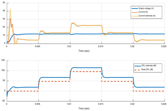
Relative to the Section 3 results shown in Figure 6 and Figure 7 for the hybrid controller (Type-III + MPC RG), Figure 8 and Figure 9 present the hybrid estimator’s transient properties. The top sub-figures show the convergence profile of the current estimator (18), while the bottom sub-figures reveal the transient behavior of the power estimator (20). Accurate and fast convergence in all cases is observed. This is the key to the successful output voltage regulation of the hybrid controller shown in Figure 6 and Figure 7.
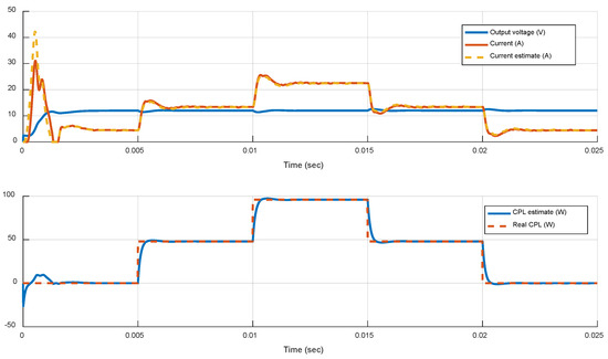
Figure 8.
Transient responses of the estimator’s convergence properties for the controller in Figure 6. The combination of PID Type III controller and MPC reference governor is evaluated for constant Vin, R, and varying CPL load in boost mode, for ratios up to 4 (96 W).
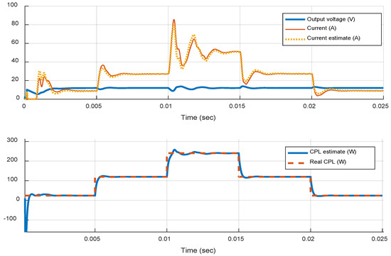
Figure 9.
Transient responses of the estimator’s convergence properties for the controller in Figure 7. The combination of PID Type III controller and MPC reference governor is evaluated for constant Vin, R, and varying CPL load in boost mode. The converter’s robustness limits are investigated with ratios Pr up to 10 (240 W).
For the two estimators used the tuning choices made are as follows: In (17) the tuning parameters are . After some experimentation with the tuning suggestions in Reference [31], appropriate values have been found for (corresponding to CVL load resistance in the designated range 6–60 Ω). Τhe value of the parameter is determined by the a priori assumed perturbation bounds of the unknown load (the CPL bounds can be also considered if desired). The choice does not take the CPL bounds a priori into account; however, the robust properties of the current estimator (as explained in the previous section) have been validated by the simulation results, as the estimator’s convergence and performance are not seriously affected. In (19) the main tuning parameter value has been used, selected to represent a reasonable trade-off between convergence rate and robustness (an estimator’s convergence rate roughly 4–5 times faster to controlled system’s settling rate is obtained).
It is important to note that the picture shown in Figure 8 and Figure 9 is an idealized one, since in (18) and (20) it is clearly assumed that the value of the resistive load is exactly known. This may be close to reality when the resistive load is negligible (only CPL loading is assumed) or it is accurately a priori known (in the absence of uncertainty). Hence, the results shown so far in Figure 6, Figure 7, Figure 8 and Figure 9 are representative of this case.
It is also true that the hybrid scheme proposed is capable of maintaining the same good robustness properties in the presence of uncertainty for the resistive load, as proved in Section 4.3. To ascertain this property, we consider the most realistic composite load case, i.e., we assume that only the nominal value is known. For an uncertain in the range 6–60 Ω (Table 1), we may assume, e.g., . With the values of in (18) and (20) replaced by the same experiments are repeated. The new simulation results are shown in Figure 10 and Figure 11. We observe that the estimator’s convergence and the controller’s performance have not been affected (the extreme ratio value, which is tolerable, remains equal to 10). The only difference is the steady-state error appearing in the power estimator (bottom sub-figures). This is expected since there is no means to add some type of integral action to this estimator; however, this does not affect the overall system performance, due to the robustness properties proved in Section 4.3. In fact, if required, the known perturbation bounds for can be used to calculate the power estimate error bounds from (19), and retune the current estimator in (17) with a modified value for the parameter , that ensures robust convergence.
5.2. The MPC RG Tuning for Tracking and Disturbance Rejection
In this subsection, we evaluate in detail the performance of the proposed scheme in several tracking and disturbance rejection tasks with composite loads. The effect of CPL loading and different tuning choices is investigated. The converter’s behavior during startup is examined separately in the following subsection. We begin by repeating some of the results presented in Reference [22] for the case of CVL loads. Then, the effect of an additional CPL load is examined.
An MPC frequency of 50 KHz and three different weighting factor values (50, 500, 1000) have been used in the simulation results shown next. Moreover, rate constraints as in (16) with = 0.5 are introduced to penalize extreme aggressiveness. The corresponding closed-form MPC gains are collected in Table 5. Smaller MPC control frequencies, e.g., 25 KHz have been also tested, however, the variability of the control signals is clearly limited in this case and although some performance improvement can still be obtained, it is notably inferior when compared with the 50 KHz case.
Table 5.
MPC RG gains for rw = 50, 500, 1000.
5.2.1. In the Absence of CPL Load (CVL Case)
It is clear from all cases in Figure 12 and Figure 13 that the PID type-III controller alone suffers from long settling times due to highly oscillatory behavior, giving also rise to large current spikes in the initial phase of the transients. The hybrid controller (PID type-III + MPC RG) provides significant improvements in terms of rise time, settling time, and overcurrent avoidance. The key to achieving this performance enhancement is the dynamic modification of the reference input by which the PID type-III controller is commanded using an MPC RG scheme. Both the inductor currents and the duty cycle waveforms shown in Figure 12 and Figure 13 reveal that the performance benefits obtained are not attributed to higher absolute values of currents or duty cycles, or extensive use of energy, but rather in a smarter use of the available energy that is characterized by higher variability. The hybrid controller appears to act in a much more flexible manner allowing large excursions of the control signals in a short time scale, without imposing extra operational requirements, e.g., higher inductor currents or energy consumption or excessive duty cycles. Smaller weighting factor values inject more flexibility and freedom in the inductor current and duty cycle waveforms, thanks to the more elaborate dynamic adjustments of the reference control signal. Over-currents can be easily dealt within this framework in a straightforward manner, i.e., by an appropriate choice of the weighting factor . We observe that in all situations the current spikes are significantly decreasing with smaller values.
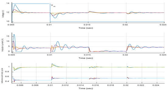
Figure 12.
Comparative transient responses of the output voltage and inductor current for a PID type-III controller with and without MPC reference governors (control factor rw = 50, 500, 1000).
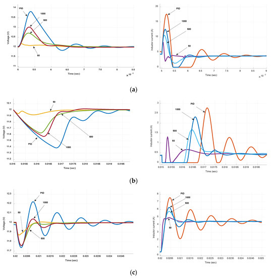
Figure 13.
Comparative transient responses (detailed view) for three of the cases of Figure 12. (a) Input voltage step change from Vin = 10 V to 14 V (Boost to Buck mode) for R = 6 Ω; (b) Input voltage step change from Vin = 14 V to 10 V (Buck to Boost mode) for R = 60 Ω; (c) Load step change (from 60 Ω to 6 Ω) in Boost mode (Vin = 10 V).
5.2.2. In the Presence of Additional CPL Load (CVL + CPL)
The benefits offered by the hybrid controller have been already described in the motivation section. The robustness improvement obtained in the presence of CPL loads is remarkable. Furthermore, all results presented so far suggest that clearly better performance is also granted in all situations, i.e., CVL, CPL, or composite (CVL + CPL) loads.
The performance of the controller for a composite load with ratios up to 4 (96 W) is studied in more detail in Figure 14 and Figure 15. Good tracking and CPL disturbance rejection is observed for all three tuning choices proposed in Table 5. Prolonged oscillations are avoided and current-voltage-duty cycle overshooting and/or settling time can be simply tuned using the correct value for , as these measures are decreasing with smaller values.
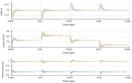
Figure 14.
Tracking and disturbance rejection of the hybrid controller, for constant Vin = 10 V, R = 6 Ω and varying CPL load in boost mode, for rw = 50, 500, 1000. Same cases as in Figure 6 (Startup case is excluded). The CPL load is stepping up and down twice, i.e., 0 → 48 W → 96 W → 48 W → 0.
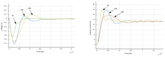
Figure 15.
Tracking and disturbance rejection output voltage and inductor current (detailed view) of the first case shown in Figure 14, i.e., a CPL load step transient for 0 → 48 W and rw = 50, 500, 1000.
5.3. Startup Considerations
To test the startup behavior, a choice has been made to experiment with the most extreme case, i.e., lightest load conditions in boost mode for the resistive load CVL (Vin = 10 V, R = 6 Ω). In the absence of any CPL loads, several startup transient responses for PID type-III and hybrid designs are compared in Figure 16. The PID type-III controller produces the fastest rise time, however, it suffers severely from an unacceptably high over-current and it also exhibits a long settling time due to oscillatory behavior. The hybrid controllers give also rise to significant over-currents, however, these spikes seem to be adjustable with a single tuning knob, as they decrease with larger rw choices.
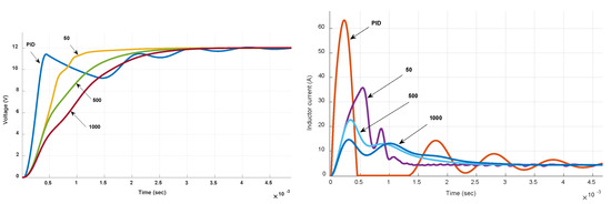
Figure 16.
Comparative startup transient responses of the output voltage for a PID type-III controller with and without MPC reference governors for control weighting factor rw = 50, 500, 1000, for an input voltage Vin = 10 V (Boost mode) and R = 6 Ω, in the absence of any CPL load.
Nevertheless, these results dictate the need for some form of soft-start procedure during startup, especially in the case that inductor currents must be maintained within some limits for safety reasons. Depending on our tolerances, a proper trade-off can be made between startup and the other operation modes. The hybrid scheme proposed can be also easily tuned to play the role of a soft-starter if required, simply by using different gains (MPC tuning) for different modes.
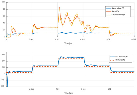
In the presence of CPLs, startup procedures are even more problematic and challenging compared to simple CVL loads. This is confirmed by repeating the previous experiment with the same CVL (24 W), while adding a variable CPL (12, 24, 48 W), for a hybrid controller with fixed rw = 500, Vin = 10 V, R = 6 Ω in boost mode. The simulation results are depicted in Figure 17 and Figure 18. We observe, in the initial phase of the response, a significant increase of inductor current spikes with a corresponding voltage collapse, before the controller can recover and bring the system to the desired set-point. Figure 18 suggests that this behavior is mainly due to the poor performance of the hybrid estimator used in the hybrid scheme, which fails to converge quickly and helps mitigating the negative impedance behavior injected by the CPL. However, this is natural and expected if there is no prior information for the initial CVL or CPL loading.
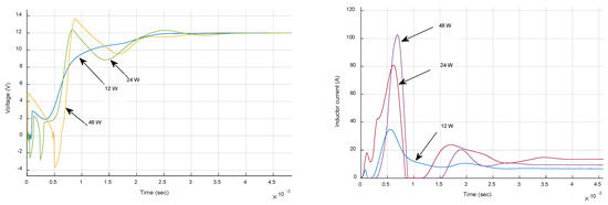
Figure 17.
Startup transient responses of the output voltage and the inductor current for the hybrid controller (PID type-III + MPC RG) for rw = 500, Vin = 10 V, R = 6 Ω, in the presence of different CPL loads 12, 24, 48 W.
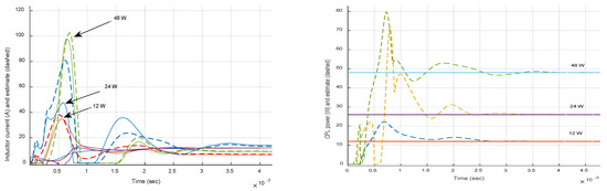
Figure 18.
The current and CPL power estimates corresponding to the cases of Figure 17. Solid curves represent the real values and dashed ones their estimates.
Hence, we conclude that, especially in the presence of unknown CPL loads, considering a carefully designed soft startup procedure is necessary, which must be separated from the main control design and tuning process explained in the previous sections. Similar Inrush current limitation designs are also discussed in several works, see, e.g., [19] and references therein, but are out of the scope of the present paper.
6. Conclusions
In recent research, hybrid controllers have been proposed for the voltage regulation of pre-compensated buck-boost DC-DC converters in uncertain resistive load conditions. Such converters can benefit from the addition of a secondary controller in the form of a reference governor that dynamically modifies the set-point of the primary controller. The proposed scheme is designed optimally via a simple linear Model Predictive Control methodology and can be implemented in an explicit form (avoiding online optimization) using a digital microprocessor. A successful design in the case of resistive loads has been demonstrated recently, which requires extra knowledge of the inductor current. This is provided by a nonlinear current observer.
The purpose of this article has been the evaluation of this recently proposed hybrid controller for a buck-boost DC-DC converter in additional uncertain CPL loading conditions. Our simulation results suggest that a PID-type III primary controller alone fails to deal with CPLs. On the contrary, the hybrid controller—designed for CVL loads—possesses good performance and robustness properties in a wide operating range also in the case of additional CPL loads, even in extreme loading conditions. This is true without having to redesign the controllers, but simply by replacing its current observer by a new hybrid observer that includes an additional CPL power estimator. These results are particularly useful in cases where the PID Type-III part of the hybrid controller is already hardcoded and cannot be changed for cost and/or safety reasons.
It has been recently argued in the literature that nonlinear (bilinear) converters of the boost or buck-boost family, especially under CPL loads, require non-linear control methodologies for large-signal stability and high performance. Our results suggest that hybrid linear control methodologies may also be suitable in this respect. Moreover, due to its two-level nature, a hybrid MPC RG controller can be also used with common pre-compensated hardware primary controllers. Finally, an MPC RG is expressed in a closed-form with constant gains, which offers a transparent digital implementation of low computational burden.
Future work will further investigate this claim in other converter types, i.e., interleaved boost or double boost topologies, and with the help of additional hardware experiments. Adaptive designs using, e.g., the estimated CPL power will be also studied.
Author Contributions
Conceptualization, C.Y.; Methodology, C.Y.; Project administration, S.V.; Software, C.Y.; Supervision, S.P.; Validation, S.P.; Writing—original draft, C.Y.; Writing—review & editing, S.P. All authors have read and agreed to the published version of the manuscript.
Funding
This research was funded by EU-funded HORIZON2020 project inteGRIDy—integrated Smart GRID Cross-Functional Solutions for Optimized Synergetic Energy Distribution, Utilization and Storage Technologies, H2020 Grant Agreement Number: 731268.
Conflicts of Interest
The authors declare no conflict of interest.
References
- Kwasinski, A.; Onwuchekwa, C.N. Dynamic Behavior and Stabilization of DC Microgrids with Instantaneous Constant-Power Loads. IEEE Trans. Power Electron. 2010, 26, 822–834. [Google Scholar] [CrossRef]
- Singh, S.; Gautam, A.R.; Fulwani, D. Constant power loads and their effects in DC distributed power systems: A review. Renew. Sustain. Energy Rev. 2017, 72, 407–421. [Google Scholar] [CrossRef]
- Barabanov, N.; Ortega, R.; Griñó, R.; Polyak, B. On Existence and Stability of Equilibria of Linear Time-Invariant Systems with Constant Power Loads. IEEE Trans. Circuits Syst. I Regul. Pap. 2015, 63, 114–121. [Google Scholar] [CrossRef]
- Olalla, C.; Leyva, R.; El Aroudi, A. Robust LQR control for PWM converters: An LMI approach. IEEE Trans. Ind. Electron. 2009, 7, 2548–2558. [Google Scholar] [CrossRef]
- Olalla, C.; Queinnec, I.; Leyva, R.; El Aroudi, A. Robust optimal control of bilinear DC–DC converters. Control Eng. Pract. 2011, 19, 688–699. [Google Scholar] [CrossRef]
- Olalla, C.; Leyva, R.; Queinnec, I.; Maksimovic, D. Robust Gain-Scheduled Control of Switched-Mode DC–DC Converters. IEEE Trans. Power Electron. 2012, 27, 3006–3019. [Google Scholar] [CrossRef]
- Yfoulis, C.; Giaouris, D.; Stergiopoulos, F.; Ziogou, C.; Voutetakis, S.; Papadopoulou, S. Robust constrained stabilization and tracking of a boost DC-DC converter through bifurcation analysis. Control Eng. Pract. 2015, 35, 67–82. [Google Scholar] [CrossRef]
- Mariéthoz, S.; Almér, S.; Bâja, M.; Beccuti, A.G.; Patino, D.; Wernrud, A.; Buisson, J.; Cormerais, H.; Geyer, T.; Fujioka, H.; et al. Comparison of Hybrid Control Techniques for Buck and Boost DC-DC Converters. IEEE Trans. Control Syst. Technol. 2009, 18, 1126–1145. [Google Scholar] [CrossRef]
- Vazquez, S.; Leon, J.I.; Franquelo, L.G.; Rodriguez, J.; Young, H.A.; Marquez, A.; Zanchetta, P. Model Predictive Control: A Review of Its Applications in Power Electronics. IEEE Ind. Electron. Mag. 2014, 8, 16–31. [Google Scholar] [CrossRef]
- Bordons, C.; Montero, C. Basic principles of MPC for power converters: Bridging the gap between theory and practice. IEEE Ind. Electron. Mag. 2015, 9, 31–43. [Google Scholar] [CrossRef]
- Kouro, S.; Perez, M.A.; Rodriguez, J.; Llor, A.M.; Young, H.A. Model predictive control: MPC’s role in the evolution of power electronics. IEEE Ind. Electron. Mag. 2015, 9, 8–21. [Google Scholar] [CrossRef]
- Beccuti, A.; Mariethoz, S.; Cliquennois, S.; Wang, S.; Morari, M. Explicit Model Predictive Control of DC–DC Switched-Mode Power Supplies with Extended Kalman Filtering. IEEE Trans. Ind. Electron. 2009, 56, 1864–1874. [Google Scholar] [CrossRef]
- Kim, S.-K.; Park, C.R.; Kim, J.; Lee, Y.I. A Stabilizing Model Predictive Controller for Voltage Regulation of a DC/DC Boost Converter. IEEE Trans. Control Syst. Technol. 2014, 22, 2016–2023. [Google Scholar] [CrossRef]
- SadAbadi, M.S.; Shafiee, Q.; Karimi, A. Plug-and-Play Robust Voltage Control of DC Microgrids. IEEE Trans. Smart Grid 2017, 9, 6886–6896. [Google Scholar] [CrossRef]
- Cucuzzella, M.; Lazzari, R.; Trip, S.; Rosti, S.; Sandroni, C.; Ferrara, A. Sliding mode voltage control of boost converters in DC microgrids. Control Eng. Pract. 2018, 73, 161–170. [Google Scholar] [CrossRef]
- Cucuzzella, M.; Lazzari, R.; Kawano, Y.; Kosaraju, K.C.; Scherpen, J.M.A. Robust Passivity-Based Control of Boost Converters in DC Microgrids. In Proceedings of the 2019 IEEE 58th Conference on Decision and Control (CDC), Nice, France, 11–13 December 2019; pp. 8435–8440. [Google Scholar] [CrossRef]
- He, W.; Ortega, R.; Machado, J.; Li, S. An adaptive passivity-based controller of a buck-boost converter with a constant power load. Asian J. Control 2019, 21, 581–595. [Google Scholar] [CrossRef]
- Singh, S.; Fulwani, D. Constant Power Loads: A solution using Sliding Mode Control. In Proceedings of the IECON 2014, Dallas, TX, USA, 29 October–1 November 2014; pp. 1989–1995. [Google Scholar]
- El Aroudi, A.; Martínez-Treviño, B.A.; Vidal-Idiarte, E.; Cid-Pastor, A. Fixed Switching Frequency Digital Sliding-Mode Control of DC-DC Power Supplies Loaded by Constant Power Loads with Inrush Current Limitation Capability. Energies 2019, 12, 1055. [Google Scholar] [CrossRef]
- Xu, Q.; Blaabjerg, F.; Zhang, C.; Yang, J.; Li, S.; Xiao, J. Xiao An Offset-free Model Predictive Controller for DC/DC Boost Converter Feeding Constant Power Loads in DC Microgrids. In Proceedings of the IECON 2019, Lisbon, Portugal, 14–17 October 2019; pp. 3905–3909. [Google Scholar]
- Yfoulis, C. An MPC Reference Governor Approach for Enhancing the Performance of Precompensated Boost DC–DC Converters. Energies 2019, 12, 563. [Google Scholar] [CrossRef]
- Yfoulis, C.; Papadopoulou, S.; Voutetakis, S. Enhanced control of a buck-boost DC-DC converter via a closed-form MPC reference governor scheme. In Proceedings of the IECON 2019, Lisbon, Portugal, 14–17 October 2019; pp. 201–206. [Google Scholar]
- Cavanini, L.; Cimini, G.; Ippoliti, G.; Bemporad, A. Model predictive control for pre-compensated voltage mode controlled DC–DC converters. IET Control Theory Appl. 2017, 11, 2514–2520. [Google Scholar] [CrossRef]
- Cavanini, L.; Cimini, G.; Ippoliti, G. Model predictive control for the reference regulation of current mode controlled dc-dc converters. In Proceedings of the2016 IEEE 14th Int. Conf. on Industrial Informatics (INDIN), Poitiers, France, 19–21 July 2016; pp. 74–79. [Google Scholar]
- Kurokawa, F.; Yamanishi, A.; Hirotaki, S. A reference modification model digitally controlled DC-DC converter for improvement of transient response. IEEE Trans. Power Electron. 2016, 31, 871–883. [Google Scholar] [CrossRef]
- Kolmanovsky, I.; Garone, E.; Di Cairano, S. Reference and command governors: A tutorial on their theory and automotive applications. In Proceedings of the 2014 American Control Conference, Institute of Electrical and Electronics Engineers (IEEE). Portland, OR, USA, 4–6 June 2014; pp. 226–241. [Google Scholar]
- Kogiso, K.; Hirata, K. Reference governor for constrained systems with time-varying references. Robot. Auton. Syst. 2009, 3, 289–295. [Google Scholar] [CrossRef]
- Jade, S.; Hellstrom, E.; Larimore, J.; Stefanopoulou, A.; Jiang, L. Reference governor for load control in a multi cylinder recompression HCCI engine. IEEE Trans. Control Syst. Technol. 2014, 22, 1408–1421. [Google Scholar] [CrossRef]
- Basso, C.P. Switch-Mode Power Supplies Spice Simulations and Practical Designs; McGraw-Hill: New York, NY, USA, 2008. [Google Scholar]
- Wang, L. Model Predictive Control System Design and Implementation Using MATLAB, Advances in Industrial Control; Springer: Berlin/Heidelberg, Germany, 2009. [Google Scholar]
- Cimini, G.; Ippoliti, G.; Orlando, G.; Longhi, S.; Miceli, R. A unified observer for robust sensorless control of DC–DC converters. Control Eng. Pract. 2017, 61, 21–27. [Google Scholar] [CrossRef]


© 2020 by the authors. Licensee MDPI, Basel, Switzerland. This article is an open access article distributed under the terms and conditions of the Creative Commons Attribution (CC BY) license (http://creativecommons.org/licenses/by/4.0/).