Abstract
The limitation of fossil fuel uses and GHG (greenhouse gases) emissions reduction are two of the main objectives of the European energy policy and global agreements that aim to contain climate changes. To this end, the building sector, responsible for important energy consumption rates, requires a significant improvement of its energetic performance, an obtainable increase of its energy efficiency and the use of renewable sources. Within this framework, in this study, we analysed the economic feasibility of a stand-alone photovoltaic (PV) plant, dimensioned in two configurations with decreasing autonomy. Their Net Present Value at the end of their life span was compared with that of the same plant in both grid-connected and storage-on-grid configurations, as well as being compared with a grid connection without PV. The analysis confirms that currently, for short distances from the grid, the most suitable PV configuration is the grid-connected one, but also that the additional use of a battery with a limited capacity (storage on grid configuration) would provide interesting savings to the user, guaranteeing a fairly energetic autonomy. Stand-alone PV systems are only convenient for the analysed site from distances of the order of 5 km, and it is worth noting that such a configuration is neither energetically nor economically sustainable due to the necessary over-dimensioning of both its generators and batteries, which generates a surplus of energy production that cannot be used elsewhere and implies a dramatic cost increase and no corresponding benefits. The results have been tested for different latitudes, confirming what we found. A future drop of both batteries’ and PV generators’ prices would let the economic side of PV stand-alone systems be reconsidered, but not their energetic one, so that their use, allowing energy exchanges, results in being more appropriate for district networks. For all PV systems, avoided emissions of both local and GHG gases (CO2) have been estimated.
1. Introduction
Today, the limitation of fossil fuel use, a major cause of the present day climate change, along with greenhouse gas emission reduction [1,2,3], represent the main energy challenges that must be faced, being fundamental aspects of international agreements (COP 2015) and EU (European Union) Directives [4,5], which are particularly addressed in order to reduce primary energy consumption and increase the share of renewable energy sources (RES) [6,7,8,9].
A significant rate of primary energy (with the associated greenhouse gas emissions) is consumed in buildings: with reference to Italy, potential savings are about 40% in energy end-use and 36% in greenhouse gases (GHG). They could be significantly reduced by adopting sustainable design, increasing energy efficiency [10,11,12,13,14] and making wider RES use [15,16,17,18,19]. Regional RES implementation examples are reported in [20,21].
Nowadays, the construction sector is in fact required to guarantee high levels of living comfort [22,23,24,25,26] with low primary energy consumption and greenhouse gases emissions, in a cost-optimal vision [27,28]: in the EU, this has allowed for the legislative implementation of the ambitious nZEB (nearly Zero Energy Building) [29,30], with a particularly high energy performance. Recent progress, future challenges and a roadmap on this matter are reported in [31,32,33].
Thanks to such increasingly challenging energy targets, the energy requalification of the building stock currently offers important opportunities for innovation [34,35,36], both concerning the envelope [37,38] and the plants. In Italy, in particular, the Italian National Energy Strategy [39,40] adopts both challenging thermal characteristics for the envelope (such as minimum transmittances) and the use of RES.
The integration of renewable energy systems with storage systems, both electrical [41,42,43] and thermal [44,45,46], would completely satisfy the energy demand, so that storage techniques, including innovative ones [47,48,49,50,51], currently represent a peculiar interest for both researchers and technicians. Anyway, the present cost of energy storage and other critical issues within the systems (over-dimensioning and energy surplus) currently make them neither energetically nor economically sustainable, unless the cost of grid connection is higher for elevated distances [52,53,54,55].
Consequently, the new energy paradigm to be established in the future would mainly be based on energy districts, nZEBs, grid-connected RES [56,57,58,59] endowed with energy storage, smart grids [60,61,62] and electric mobility [63,64], rather than on completely autonomous renewable systems.
To this end, in this paper we analysed different configurations of PV plants in a residential building (grid-connected, storage-on-grid and stand-alone) in terms of energy rates, costs and emission reductions, as a function of the distance from the grid.
The main aim of the study is the evaluation of the current cost of building energetic self-sufficiency and thus of user independency in the national electric network. As mentioned above, the use of stand-alone PV systems is not in fact sustainable, as both their generators and batteries must be dimensioned so as to guarantee an energy load in the worst condition, which is to say on the day of the year with the least daylight and energy production (i.e., winter solstice), which requires PV generators and batteries with an overflowing power and capacity: this implies a dramatic cost increase and no corresponding benefits for most months of the year, as it is not possible to use the respective surplus of energy production elsewhere. This means that PV stand-alone configurations are, in general, not advisable, apart from in isolated areas where the cost of a grid connection would result in being greater that of an autonomous system.
The most suitable system is, on the contrary, a grid-connected configuration [65], also using a battery of limited capacity, with no PV generator over-dimensioning, which therefore markedly reduces the system cost, allowing an energy surplus sale and its purchase within only months, with minimum irradiation. This concern about PV systems is not markedly underlined in the literature.
Within this field, the case study compares the energy rates, costs and avoided emissions of a stand-alone PV system located in the Italian city of Reggio Calabria, dimensioned in two different configurations with decreasing autonomy (and the consequent power and cost), guaranteeing a load for one or two days respectively, with those of both a grid-connected configuration of the same plant, also endowed with a small battery (storage on grid), and a simple connection to the grid (Figure 1) as a function of the distance from the grid.
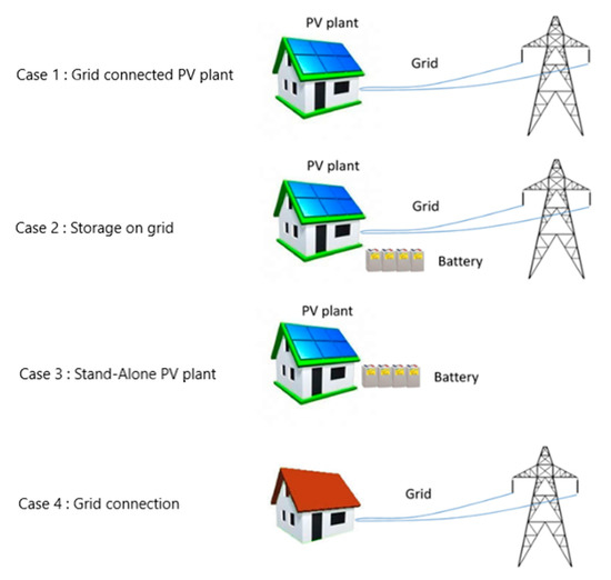
Figure 1.
Assessed patterns of power supply.
To compare the five configurations, their Net Present Value was evaluated at the end of the plant life, identifying the relative cost/benefit items (the latter assessed on the basis of the Italian Government incentivizing fares), and the drawn vs. distance from the grid.
The analysis has been conducted by setting the same case study in three Italian areas with different latitudes (and therefore different irradiations), showing the same results.
Moreover, for all PV configurations, the avoided emissions of both GHG (CO2) and local pollutants (NOx, SO2, PM10) have been estimated.
2. PV System Sizing
2.1. Daily Load Assessment
The electric energy daily demand (D), simulated using the software PVSol (PV*Sol 2020 R7, Valentine Software GmbH, Stralauer Platz 34, 10243 Berlin, Germany) (by Valentine Software German company), was assessed in order to determine the yearly load, in order to size up both the nominal power of the PV array and, when present, the battery capacity. Further information required in order to dimension the stand-alone generator was the daily maximum load in the year.
2.2. Solar Irradiance on the Panels
The purpose of this step is the maximization of solar irradiance striking the panels’ surfaces, corresponding to an optimal orientation and tilt angle at the site’s latitude. Starting from the values of solar irradiation on the horizontal surface of the site (UNI 10349 [66]), the corresponding values on panel’s surface, I, have been derived.
2.3. Nominal Power Assessment–Grid-Connected and Storage-on-Grid PV plant
The peak power of the grid-connected PV systems was estimated on the basis of the user consumption and solar irradiation in the site. It has been assessed by referring to the peak solar hours teq, the equivalent period of time with a constant irradiance Is = 1 kW/m2 providing the same actual radiation I (kWh/m2) striking the module’s surface [67]:
The nominal power delivered by the PV array in the absence of power losses Pid is calculated as:
where D is the yearly energy demand.
The nominal power under the real condition P, considering power losses in the PV system (depending on cell temperatures, shading effects, solar radiation reflections, dirt on module surfaces, etc.) and in its electronic devices (inverter, batteries, charge regulator, link cables, etc.) is then calculated as:
where η is the system’s overall efficiency.
2.4. Nominal Power Assessment–Stand-Alone PV Plant
Stand-alone systems must provide power to loads, even when solar irradiance is insufficient or during night time: during such periods, batteries must support the generation system, so their proper capacity must be sized up.
The power of the PV array must consequently be determined so that during sunshine periods it can allow both load feeding and battery charging. The energy that is to be delivered daily and stored in batteries is a function of the number N of autonomy days of the system and of the load to satisfy.
Two different configurations, with increasing autonomy (referred to as case a and case b), have been considered. The maximum user’s daily demand, Dmax, is to be guaranteed for one day (N = 1) in case a and for two days (N = 2) in case b.
The nominal power of the PV array in the absence of power losses Pid that is able to generate the energy required to meet the load and completely charge the battery is given by:
where t*eq are the equivalent hours of the minimum irradiance day (21st December). The nominal power under the real condition P is subsequently obtained from Equation (3).
2.5. Battery Sizing
The battery capacity Ca is:
where:
- Dd is the design load,
- V is the rated voltage of the array (V),
- Lc is the minimum allowed depth of the battery discharge (%).
2.6. Charge Controller Dimensioning
In stand-alone and storage-on-grid systems, an essential component for their operation and lifetime is the charge controller, which adjusts the energy flow and protects batteries from an insufficient or excessive charge, increasing their life. Its selection depends on the maximum producible current from the PV field:
with n being the number of strings and Icc,module the short circuit current.
2.7. Shadows Pattern
The shadow patterns of the installation site are fundamental for the sizing procedure; they can both reduce solar irradiance on panels and produce dissymmetry within their operation, modifying the solar irradiance profiles and strictly affecting the system arrangement. To this end, knowledge of the yearly sun paths at the site’s latitude is required.
The string distance d, minimizing reciprocal shadows, has been determined assuming that it avoids shadows in the worst case, that is on 21 December (winter solstice) at 12 a.m. [68]:
where:
- L module installation height (m),
- δ module tilt (°),
- α sun altitude at 12 a.m. on 21 December (°).
3. Energy Production
The energy production E has been determined with an hourly step through PVSol software using the following equation:
where
- η panel efficiency,
- S panels surface (m2),
- I solar irradiance on the panel (kWh/m2),
- η is a function of the temperature (it decreases as the temperature increases):
- ηr panel efficiency at reference temperature,
- β panel temperature coefficient (%/°C),
- tc cell temperature (°C),
- tr reference temperature (25 °C).
The cell temperature is estimated using the expression:
where
ta air temperature (°C),
NOCT Nominal Operating Cell Temperature (°C),
Is solar radiation power on the panel (W/m2).
4. Case Study
The described methodology has been applied to a residential user, placed in Reggio Calabria (38°06’ N, 15°39’ E) in the South of Italy. The generator lies facing south, inclined at 28° (optimal inclination for the site). No shadows are present over the PV system in order to consider the most general case.
The load profile is reported in Figure 2; the total yearly demand is 3035 kWh.
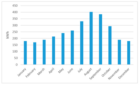
Figure 2.
Electric energy load.
For the presence of an energy-consuming air conditioning system, the maximum load is observed in summer, whereas the lower demand in winter is due to the use of a gas boiler for heating purposes.
4.1. PV System Sizing
The UNI 10349 standard provides the values of the monthly average solar irradiation on a horizontal surface for the city of Reggio Calabria; from these, the corresponding values on the generator surface facing south, inclined at 28°, have been derived (Figure 3).
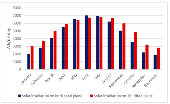
Figure 3.
Monthly solar irradiation in Reggio Calabria.
The selected PV modules are in monocrystalline silicon, with an efficiency of 0.205, and have a module power Pm = 280 Wp.
4.1.1. Case 1: Grid-Connected PV System
Using Equation (3), the value of the peak power of the plant has been obtained (2.1 kWp). The minimum number of modules is:
For the conversion DC/AC, an inverter has been inserted, selecting a pure sine wave one; it has a 2.8 kW power, assessed on the basis of the maximum absorption.
In Figure 4, a schematic representation of the PV systems is reported. The panels are arranged in two strings of four modules each; the distance between the modules is 3.38 m, calculated by Equation (7).
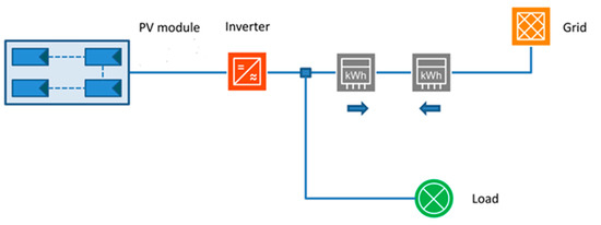
Figure 4.
Schematic representation of the grid-connected PV system.
4.1.2. Case 2: Storage-on-Grid PV System
This represents an intermediate case, realised with a grid-connected plant equipped with a battery pack dimensioned only so as to satisfy the average night load (4 kWh/day), without the necessity of returning to the national grid. Consequently, the generator power, the number of panels and their arrangement in strings, together with the inverter characteristics, are the same as the grid-connected configuration. In Figure 5, a schematic representation of the configuration is reported.
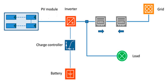
Figure 5.
Schematic representation of the storage on the grid PV system.
The batteries have a gel electrolyte, 12 V voltage and a capacity of 4.8 kWh, considering a minimum discharge level of 20%. From (5), the capacity in Ah results in:
An acid control valve allows for a long duration (average lifetime over 10 years), with no maintenance.
4.1.3. Case 3: Stand-Alone System
In the case of stand-alone systems with no grid support, a failure of energy occurring particularly in winter due to insufficient sunlight must be avoided by increasing the plant power in order to store part of the energy production. To this end, the determinations of both the daily maximum consumption in the year Dmax (13.1 kWh) and the minimum number of peak solar hours (2.7 h) are necessary.
If only a day’s autonomy is to be guaranteed (N = 1, case a), Equation (4) provides:
Assuming an overall plant efficiency equal to 0.8, its peak power P results in:
and the minimum number of modules to be installed is:
Two arrays of 22 modules each connected in parallel have been chosen. The distance between the modules is unvaried with respect to the grid-connected configuration. The load being unvaried, the same inverter as for the grid-connected case has been adopted.
The batteries for energy storage have a 7.6 kWh capacity. In order to guarantee the demand, two batteries with a capacity of 1365 Ah are required.
As for the charge controller, given that we have from (6). Four charge controllers, connected in parallel, have been adopted, allowing a 40 A input current each.
When considering two days of autonomy (N = 2, case b), we have a peak power of 18.2 kWp, and the number of panels to install is 66, arranged in six arrays of 11 that are connected in parallel and are spaced as in previous configurations.
The storage capacity is higher, requiring four batteries. As for the charge controllers, for 66 modules, a maximum producible current of 50 A is obtained: six controllers have been used, allowing a 50 A input current each.
In Figure 6, a scheme of the configured stand-alone system is represented.
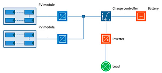
Figure 6.
Schematic representation of the stand-alone PV system.
4.1.4. Case 4: Connection to the Grid
In order to evaluate the economic convenience of the configured systems, a comparison of their cost with that resulting from a simple connection to the electric grid has been conducted.
5. Energetic Analysis
The energetic behaviour of the plant typologies has been simulated with an hourly step using PV-Sol software.
In Figure 7, referring to the grid-connected configuration, the energy production and energy shares (directly used energy, grid intake and energy provided by the grid) are reported. Further information that can be drawn from the figure are the load and energy production:
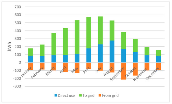
Figure 7.
Monthly energy flows for the grid-connected PV configuration.
- load = direct use + from grid
- produced energy = direct use + to grid
Similarly, in Figure 8, referring to the storage-on-grid configuration, the energy production and energy shares (directly used energy, energy stock in batteries, grid intake of surplus and energy provided by the grid) are reported.
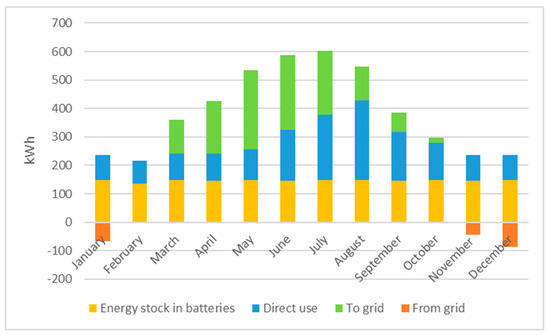
Figure 8.
Monthly energy flows for the storage-on-grid PV configuration.
Further information that can be drawn from the figure are the load and energy production:
- load = direct use + battery withdrawal + from grid
- produced energy = direct use + battery income + to grid
From an energetic point of view, the presence of the battery leads to a reduction of the energy withdrawn from the grid and at the same time a lower energy exported to the grid.
Finally, in Figure 9 and Figure 10, the energy production shares (load, battery recharge and over-production) are reported with reference to the two stand-alone configurations. From the figures, it is possible to draw the following information:
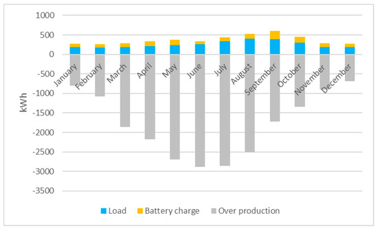
Figure 9.
Energy flows for the stand-alone PV configuration (case a).
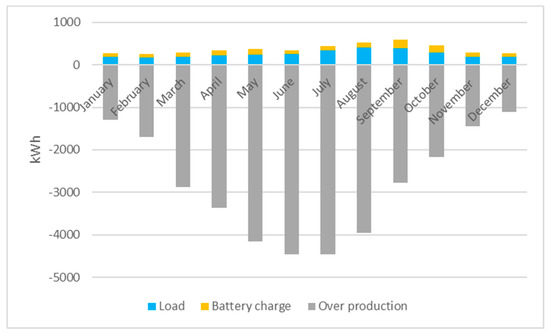
Figure 10.
Energy flows for the stand-alone PV configuration (case b).
- produced energy = load + battery charge + over production
As one can note, in stand-alone configurations, the production amply satisfies both the load and battery recharge needs; obviously, such sizing conditions markedly increase the system cost and over-production, which is equal to 21,496 kWh in case a and appreciably higher, at 33,762 kWh, in case b.
6. Economic Analysis
In order to assess the financial viability of the alternative configurations, an economic analysis was carried out through the assessment of the indicator Net Present Value (NPV), defined as:
where:
- k year,
- C annual operating costs,
- B annual benefits,
- I investment costs,
- r annual return rate.
which has been calculated vs. grid distance and is the particular parameter used in order to determine the economic convenience of the different choices.
For each case, the main cost/benefit items [69] have been identified, referring to both investment and annual operating costs (Table 1) and to income tax deduction and on-site exchange benefits provided by the Italian Government [70] (Table 2).

Table 1.
Investment and operating costs.
Table 2.
Benefits.
Generally, the investment cost is entirely supported at the beginning of the plant life, but PV plants also include inverters and other components (the stand-alone also includes batteries), whose economic life is usually smaller.
Given that an inverter’s average life is about five years, it needs to be replaced three times during the plant’s life (25 years); batteries, being a long-lasting type, are supposed to be replaced once.
In contrast, in the grid connection, the most relevant burden consists of the connection cost, given as the sum of a fixed cost and a variable one, as a function of the power that is available and of the distance. Both of these costs are given by ARERA (Authority for the Regulation of Energy, Grids and Environment) [71], and their sum is shown in Figure 11.
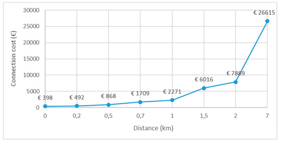
Figure 11.
Grid connection cost vs. distance.
The benefits refer to both the investment cost, with an income tax deduction equal to 50% of the initial cost, and to the energy purchase, for which an on-site exchange mechanism allows for an in-taken energy surplus to be drawn from the grid in periods of PV production lack. The cost items are reported in Table 3 and Table 4 [72,73], whereas the benefits are shown in Table 5.
Table 3.
Investment costs.
Table 4.
Annual operating costs.
Table 5.
Annual benefits.
As concerns the interest rate provided by the Bank of Italy, in accordance with the methods specified by the Special Data Dissemination Standard (SDDS) and promoted by the International Monetary Fund [74], a value of 0.69% has been assumed [75].
The diagram in Figure 12 reports NPV vs. grid distance.
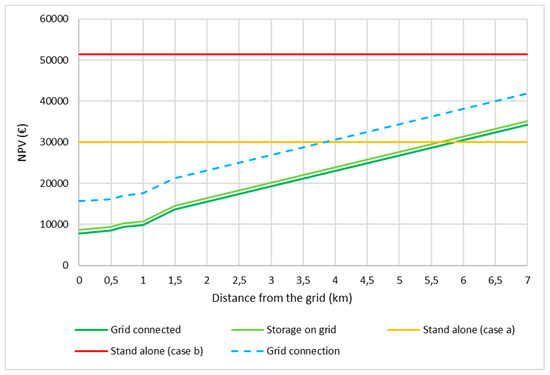
Figure 12.
NPV of the configurations.
It can be seen that, relative to the five configurations, NPV functions show intersection points, for given distances from the grid, at which their total cost is equal.
In particular, the analysis points out the existence of two critical distances (4 km and 5.7 km): below 5.7 km, the cheapest PV configurations result in being both of the grid-connected ones, which show almost the same trend, whereas over such a distance the stand-alone with a lower autonomy (case a) becomes the most convenient; in contrast, the stand-alone case b is never convenient due to the high cost of its batteries.
A further result is that the two grid-connected plants are cheaper than the grid connection for any distance from the grid, which, starting from 4 km, becomes even more expensive than the stand-alone case a.
7. Environmental Analysis
An environmental analysis was conducted considering the pollutant emissions that, on the basis of the adopted RES plants, can be avoided, with respect to an equivalent energy production provided by traditional fossil fuels.
The energy amount that is referred to is only the used part (load) of the whole PV production in the case of stand-alone plants and the shares that are directly used plus the grid in-taken shares in the case of the grid-connected ones.
Table 6 and Table 7 show, respectively, the emission factors of the main pollutants generated during the combustion of fossil fuels both with global and local effects, and the avoided emissions by analysed plant.
Table 6.
Emission factors, reproduced from [76], ISPRA 2018.
Table 7.
Avoided emissions.
Particularly concerning CO2 emissions, it can be observed that stand alone configuration allows to avoid 0.92 t/year, whereas the two grid connected ones 1.36 t/year.
8. Discussion of Main Results and Achievements
The analysis has shown that the use of stand-alone PV systems is only convenient for the analysed site (it has also been verified for different latitudes) from distances of the order of 5.7 km, confirming that such a configuration is neither energetically nor economically sustainable, requiring both its generator and batteries to be over-dimensioned (with an overflowing power and capacity, respectively) in order to satisfy the worst conditions, which occur on the winter solstice on the day of the year with the least daylight and energy production.
This implies a dramatic cost increase and no corresponding benefits during most months of the year: the surplus of energy production present during these months cannot, in fact, be used elsewhere, but must be dispersed; moreover, batteries are only filled to their maximum level during a few months of the year.
The result, according to which PV stand-alone configurations are in general not advisable, apart from in isolated areas where the cost of a grid connection would result in being greater that of an autonomous system, can be extended to other geographical areas, but the peculiarity of the critical distances which make PV stand-alone configurations convenient should be further analysed.
On the contrary, the most suitable system, at the moment, would use a grid-connected configuration, allowing for an energy surplus sale and its purchase within only months, with minimum irradiation; it is even endowed with a battery with a limited capacity, markedly reducing the system cost. Moreover, for any distance from the grid, it always results in being cheaper than the grid connection without PV.
A future drop of both battery and PV generator prices, indispensable for a RES market extension, would allow for the economic aspect of PV stand-alone systems to be reconsidered, but not their energetic aspect, so that their use could be preferably evaluated in district networks, allowing for energy exchanges.
9. Conclusions
The integration of RES plants with energy storage systems allows for the satisfactory guarantee of energy demands in buildings, with different costs depending on the presence of a grid connection or batteries so as to satisfy production lacks.
In order to evaluate the current cost of energetic self-sufficiency in buildings, in this paper a case study analyses the economic feasibility, as a function of the distance from the grid, of a stand-alone photovoltaic plant located in the Italian site of Reggio Calabria, and which is designed through two configurations with different autonomies (guaranteeing, respectively, a load for one or two days); this is compared to the same plant in a grid-connected configuration, which is also endowed with a small battery (storage on grid), and to a grid connection in the absence of PV. In fact, stand-alone configurations, due to high investment costs, are currently disadvantaged; nevertheless, they can become convenient as the distance from the grid increases.
The energetic behaviour of the plant typologies has been simulated with an hourly step, allowing for an energetic, environmental and economic assessment, the latter being evaluated through the Net Present Value, which previously identified the respective main cost/benefit items.
The analysis has shown that the use of stand-alone PV systems is only convenient for the analysed site (and was confirmed for two different Italian latitudes) from distances higher than 5 km (5.7 km) and with a one-day autonomy, confirming that such a configuration is neither energetically nor economically sustainable (given that both its generator and batteries are over-dimensioned, respectively, with an overflowing power and capacity) for satisfying loads during the worst conditions, which occur on the winter solstice on the day of the year with the least daylight and energy production. This implies a dramatic cost increase and no corresponding benefits during most months of the year: the surplus of energy production present during these months cannot, in fact, be used elsewhere, but must be dispersed; moreover, batteries are only filled to their maximum level during a few months of the year.
A future drop of both battery and PV generator prices, indispensable for a RES market extension, would allow the economic aspect of PV stand-alone systems to be reconsidered, but not their energetic aspect, so that their use could be preferably evaluated in district networks, allowing for energy exchanges.
On the contrary, the most suitable system, at the moment, would use a grid-connected configuration only allowing for an energy surplus sale and its purchase during months with a minimum irradiation and also endowed with a low-capacity battery to reduce the grid dependence (storage on grid), thus markedly reducing the system cost. Such a configuration is also more convenient than a grid connection without PV for any distance, as from a 4-km distance the latter also becomes more expensive than the previous stand-alone configuration.
A further result of the analysis is the environmental benefit provided by all of the plants, which in particular allow one to avoid more than 15 tCO2/year.
Author Contributions
Methodology A.N.; software, M.F.P.; data curation, C.M.; writing: A.P.; review and editing, M.P.; funding acquisition, M.P. All authors have read and agreed to the published version of the manuscript.
Funding
This research was funded by the Italian Ministry of Education, University and Research, grant number n. 201594LT3F, within the research project “Research for SEAP: a platform for municipalities taking part in the Covenant of Mayors”, PRIN (Programmi di Ricerca Scientifica di Rilevante Interesse Nazionale) program, https://bandi.miur.it/bandi.php/public/fellowship/id_fellow/143962.
Conflicts of Interest
Authors declare no conflict of interest.
Nomenclature
| teq | equivalent period of time with constant irradiance |
| I | irradiance |
| Is | solar radiation power on the panel |
| Pid | nominal power delivered by the PV array in the absence of power losses |
| D | yearly energy demand |
| P | nominal power under real condition |
| η | system overall efficiency |
| Dmax | maximum daily load |
| N | autonomy days of the system |
| t*eq | equivalent hours of the minimum irradiance day |
| D’max | maximum evening load |
| C | battery capacity |
| V | rated voltage of the array |
| Lc | minimum allowed depth of battery discharge |
| Imax | maximum producible current from the PV field |
| n | number of modules |
| Icc,module max | short circuit current |
| d | string distance minimizing reciprocal shadows |
| L | module installation height |
| δ | module tilt |
| α | sun altitude at 12 a.m. on 21 December |
| E | energy production |
| S | panels surface |
| ηr | panel efficiency at reference temperature |
| β | panel temperature coefficient |
| tc | cell temperature |
| tr | reference temperature |
| ta | air temperature |
| NOCT | Nominal Operating Cell Temperature |
| Pm | module power |
| NPV | Net Present Value |
| k | year |
| C | annual operating costs |
| B | annual benefits |
| I | investment costs |
| r | an |
References
- Apergis, N.; Payne, J.E. CO2 emissions, energy usage, and output in Central America. Energy Policy 2009, 35, 4772–4778. [Google Scholar] [CrossRef]
- Birge, D.; Bergera, A.M. Transitioning to low-carbon suburbs in hot-arid regions: A case-study of Emirati villas in Abu Dhabi. Build. Env. 2018, 147, 77–96. [Google Scholar] [CrossRef]
- Arsalis, A.; Alexandrou, A.N.; Georghiou, G.E. Thermoeconomic modelling of a completely autonomous, zero-emission photovoltaic system with hydrogen storage for residential applications. Renew. Energy 2018, 126, 354–369. [Google Scholar] [CrossRef]
- Official Journal of European Union. Directive 2009/28/EC of the European Parliament and of the Council of 23 April 2009, On the promotion of the use of energy from renewable sources and amending and subsequently repealing Directives 2001/77/EC and 2003/30/EC. Off. J. Eur. Union 2009, 11, 39–85. [Google Scholar]
- Official Journal of European Union. Directive 2010/31/EC of the European Parliament and of the Council of 19 May 2010, Energy performance of buildings. Off. J. Eur. Union 2010, 3, 124–146. [Google Scholar]
- Narayanan, A.; Mets, K.; Strobbe, M.; Develder, C. Feasibility of 100% renewable energy-based electricity production for cities with storage and flexibility. Renew. Energy 2019, 134, 698–709. [Google Scholar] [CrossRef]
- Foley, A.; Olabi, A.G. Renewable energy technology developments, trends and policy implications that can underpin the drive for global climate change. Renew. Sustain. Energy Rev. 2017, 68, 1112–1114. [Google Scholar] [CrossRef]
- Gonçalves da Silva, C. Renewable energies: Choosing the best options. Energy 2010, 35, 3179–3193. [Google Scholar] [CrossRef]
- Hvelplund, F. Renewable energy and the need for local energy markets. Energy 2006, 31, 2293–2302. [Google Scholar] [CrossRef]
- Official Journal of European Union. Directive 2006/32/EC of the European Parliament and of the Council of 5 April 2006, Efficiency in the final use of energy and energy systems. Off. J. Eur. Union 2006, 2, 222–243. [Google Scholar]
- Official Journal of European Union. Directive 2012/27/EC of the European Parliament and of the Council of 25 October 2012, Energy efficiency. Off. J. Eur. Union 2012, 2, 202–257. [Google Scholar]
- D’Agostino, D.; Cuniberti, B.; Bertoldi, P. Energy consumption and efficiency technology measures in European non-residential buildings. Energy Build. 2017, 153, 72–86. [Google Scholar] [CrossRef]
- Marino, C.; Nucara, A.; Pietrafesa, M. Does window-to-wall ratio have a significant effect on the energy consumption of buildings? A parametric analysis in Italian climate conditions. J. Build. Eng. 2017, 13, 169–183. [Google Scholar] [CrossRef]
- Murano, G.; Corgnati, S.P.; Cotana, F.; D’Oca, S.; Pisello, A.L.; Rossi, F. A Cost-Effective Human-Based Energy-Retrofitting Approach, Cost-Effective Energy Efficient Building Retrofitting. Mater. Technol. Optim. Case Stud. 2017, 219–255. [Google Scholar] [CrossRef]
- Parida, B.; Iniyan, S.; Goic, R. A review of solar photovoltaic technologies. Renew. Sustain. Energy Rev. 2011, 15, 1625–1636. [Google Scholar] [CrossRef]
- Razykov, T.M.; Ferekides, C.S.; Morel, D.; Stefanakos, E.; Ullal, H.S.; Upadhyaya, H.M. Solar photovoltaic electricity: Current status and future prospects. Solar Energy 2011, 85, 1580–1608. [Google Scholar] [CrossRef]
- Cotana, F.; Rossi, F.; Nicolini, A. Evaluation and optimization of an innovative Low-Cost photovoltaic solar concentrator. Int. J. Photoenergy 2011. [Google Scholar] [CrossRef]
- Malara, A.; Marino, C.; Nucara, A.; Pietrafesa, M.; Scopelliti, F.; Streva, G. Energetic and economic analysis of shading effects on PV panels energy production. Int. J. Heat Technol. 2016, 34, 465–472. [Google Scholar] [CrossRef]
- Vad Mathiesen, B.; Duić, N.; Stadler, I.; Rizzo, G.; Guzović, Z. The interaction between intermittent renewable energy and the electricity, heating and transport sectors. Energy 2012, 48, 406–414. [Google Scholar] [CrossRef]
- Kyriakopoulos, G.; Arabatzis, G.; Tsialis, P.; Ioannou, K. Electricity consumption and RES plants in Greece: Typologies of regional units. Renew. Energy 2018, 127, 134–144. [Google Scholar] [CrossRef]
- Lund, H. The implementation of renewable energy systems. Lessons learned from the Danish case. Energy 2010, 35, 4003–4009. [Google Scholar] [CrossRef]
- Marino, C.; Nucara, A.; Pietrafesa, M. Proposal of comfort classification indexes suitable for both single environments and whole buildings. Build. Environ. 2012, 57, 58–67. [Google Scholar] [CrossRef]
- Kotopouleas, A.; Nikolopoulou, M. Evaluation of comfort conditions in airport terminal buildings. Build. Environ. 2017, 130, 162–178. [Google Scholar] [CrossRef]
- Luoa, M.; Cao, B.; Zouy, X.; Li, M.; Zhang, J.; Ouyang, Q.; Zhu, Y. Can personal control influence human thermal comfort? A field study in residential buildings in China in winter. Energy Build. 2013, 72, 411–418. [Google Scholar] [CrossRef]
- Marino, C.; Nucara, A.; Pietrafesa, M. Thermal comfort in indoor environment: Effect of the solar radiation on the radiant temperature asymmetry. Solar Energy 2017, 144, 295–309. [Google Scholar] [CrossRef]
- Marino, C.; Nucara, A.; Peri, G.; Pietrafesa, M.; Pudano, A.; Rizzo, G. A MAS-based subjective model for indoor adaptive thermal comfort. Sci. Technol. Built Environ. 2015, 21, 114–125. [Google Scholar] [CrossRef]
- Guazzi, G.; Bellazzi, A.; Meroni, I.; Magrini, A. Refurbishment design through cost-optimal methodology: The case study of a social housing in the northern Italy. Int. J. Heat Technol. 2017, 35, S336–S344. [Google Scholar] [CrossRef]
- Piccolo, A.; Marino, C.; Nucara, A.; Pietrafesa, M. Energy performance of an electrochromic switchable glazing: Experimental and computational assessments. Energy Build. 2018, 165, 390–398. [Google Scholar] [CrossRef]
- Marszal, A.J.; Heiselberg, P.; Bourrelle, J.S.; Musall, E.; Voss, K.; Sartori, I.; Napolitano, A. Zero Energy Building—A review of definitions and calculation methodologies. Energy Build. 2011, 43, 971–979. [Google Scholar] [CrossRef]
- Sartori, I.; Napolitano, A.; Voss, K. Net zero energy buildings: A consistent definition framework. Energy Build. 2012, 48, 220–232. [Google Scholar] [CrossRef]
- Kapsalaki, M.; Leal, V. Recent progress on net zero energy buildings. Adv. Build. Energy Res. 2011, 5, 129–162. [Google Scholar] [CrossRef]
- Attia, S.; Eleftheriou, P.; Xeni, F.; Morlot, R.; Ménézo, C.; Kostopoulos, V.; Betsi, M.; Kalaitzoglou, I.; Pagliano, L.; Cellura, M.; et al. Overview and future challenges of nearly Zero Energy Buildings (nZEB) design in Southern Europe. Energy Build. 2017, 155, 439–458. [Google Scholar] [CrossRef]
- Kolokotsa, D.; Rovas, D.; Kosmatopoulos, E.; Kalaitzakis, K. A roadmap towards intelligent net zero-and positive-energy buildings. Solar Energy 2011, 85, 3067–3084. [Google Scholar] [CrossRef]
- AbuGrain, M.Y.; Alibaba, H.Z. Optimizing existing multistory building designs towards net-zero energy. Sustainability 2017, 9, 399. [Google Scholar] [CrossRef]
- Lund, H.; Marszal, A.; Heiselberg, P. Zero energy buildings and mismatch compensation factors. Energy Build. 2011, 43, 1646–1654. [Google Scholar] [CrossRef]
- Ballarini, I.; Dirutigliano, D.; Primo, E.; Corrado, V. The significant imbalance of nZEB energy need for heating and cooling in Italian climatic zones. Energy Procedia 2017, 126, 258–265. [Google Scholar] [CrossRef]
- Romano, R.; Gallo, P. The SELFIE Project Smart and efficient envelope’ system for nearly zero energy buildings in the Mediterranean Area. GSTF J. Eng. Technol. 2018, 4, 562–569. [Google Scholar] [CrossRef]
- Trombetta, C.; Milardi, M. Building future Lab: A great infrastructure for testing. Energy Procedia 2015, 78, 657–662. [Google Scholar] [CrossRef]
- Ministero dello Sviluppo Economico e Ministero dell’Ambiente, della Tutela del territorio e del Mare – Strategia Energetica Nazionale (SEN). 2017. Available online: https://www.mise.gov.it/images/stories/documenti/Testo-integrale-SEN-2017.pdf (accessed on 10 July 2020).
- Ministero dello Sviluppo Economico, Ministero dell’Ambiente, della Tutela del territorio e del Mare e Ministero delle Infrastrutture e dei Trasporti–Piano Nazionale Integrato per l’Energia e per il Clima. 2019. Available online: https://www.mise.gov.it/images/stories/documenti/PNIEC_finale_17012020.pdf (accessed on 10 July 2020).
- Beaudin, M.; Zareipour, H.; Schellenberglabe, A.; Rosehart, W. Energy storage for mitigating the variability of renewable electricity sources: An updated review. Energy Sustain. Dev. 2010, 14, 302–314. [Google Scholar] [CrossRef]
- Pearre, N.S.; Swan, L.G. Renewable electricity and energy storage to permit retirement of coal-fired generators in Nova Scotia. Sustain. Energy Technol. Assess. 2013, 1, 44–53. [Google Scholar] [CrossRef]
- Lorestani, A.; Ardehali, M.M. Optimization of autonomous combined heat and power system including PVT, WT, storages, and electric heat utilizing novel evolutionary particle swarm optimization algorithm. Renew. Energy 2018, 119, 490–503. [Google Scholar] [CrossRef]
- Cammarata, G.; Monaco, L.; Cammarata, L.; Petrone, G. A numerical procedure for PCM thermal storage design in solar plants. In Proceedings of the 7th AIGE Conference, Cosenza, Italy, 10–11 June 2013. [Google Scholar]
- Sharma, A.; Tyagi, V.V.; Chen, C.R.; Buddhi, D. Review on thermal energy storage with phase change materials and applications. Renew. Sustain. Energy Rev. 2009, 13, 318–345. [Google Scholar] [CrossRef]
- Lopez-Sabiron, A.M.; Royo, P.; Ferreira, V.J.; Aranda-Uson, A.; Ferreira, G. Carbon footprint of a thermal energy storage system using phase change materials for industrial energy recovery to reduce the fossil fuel consumption. Appl. Energy 2014, 135, 616–624. [Google Scholar] [CrossRef]
- Marino, C.; Nucara, A.; Pietrafesa, M.; Pudano, A. An energy self-sufficient public building using integrated renewable sources and hydrogen storage. Energy 2013, 57, 95–105. [Google Scholar] [CrossRef]
- Avril, S.; Arnaud, G.; Florentin, A.; Vinard, M. Multi-objective optimization of batteries and hydrogen storage technologies for remote photovoltaic systems. Energy 2010, 35, 5300–5308. [Google Scholar] [CrossRef]
- Marino, C.; Nucara, A.; Pietrafesa, M. Electrolytic hydrogen production from renewable source, storage and reconversion in fuel cells: The system of the Mediterranea University of Reggio Calabria. Energy Procedia 2015, 78, 818–823. [Google Scholar] [CrossRef]
- Krajacic, G.; Loncar, D.; Duic, N.; Zeljko, M.; Arantegui, R.L.; Loisel, R.; Raguzin, I. Analysis of financial mechanisms in support to new pumped hydropower storage projects in Croatia. Appl. Energy 2013, 101, 161–171. [Google Scholar] [CrossRef]
- Foley, A.; Lobera, D. Impacts of compressed air energy storage plant on an electricity market with a large renewable energy portfolio. Energy 2013, 57, 85–94. [Google Scholar] [CrossRef]
- Al-akayshee, A.S.; Kuznetsov, O.N.; Sultan, H.M. Viability Analysis of Large Photovoltaic Power Plants as a Solution of Power Shortage in Iraq. In Proceedings of the 2020 IEEE Conference of Russian Young Researchers in Electrical and Electronic Engineering (EIConRus), St. Petersburg and Moscow, Russia, 27–30 January 2020. [Google Scholar] [CrossRef]
- Yang, Y.; Lian, C.; Ma, C.; Zhang, Y. Research on Energy Storage Optimization for Large-Scale PV Power Stations under Given Long-Distance Delivery Mode. Energies 2020, 13, 27. [Google Scholar] [CrossRef]
- Bernal, E.A.; Lopez, M.B.; Ardila, A. Solar Microgrids to Enhance Electricity Access in Remote Rural Areas. 2019. Available online: https://www.researchgate.net/publication/335430858_Solar_Microgrids_to_Enhance_Electricity_Access_in_Remote_Rural_Areas (accessed on 10 July 2020).
- Nwaigwe, K.N.; Mutabilwa, P.; Dintwa, E. An overview of solar power (PV systems) integration into electricity grids. Mater. Sci. Energy Technol. 2019, 629–633. [Google Scholar] [CrossRef]
- Kaviani, A.K.; Baghaee, H.R. Gholam Hossein Riahy, Optimal Sizing of a Stand-alone Wind/Photovoltaic Generation Unit using Particle Swarm Optimization. Soc. Modeling Simul. Int. 2009, 85. [Google Scholar] [CrossRef]
- Barbaro, G.; Foti, G.; Labarbera, F.; Pietrafesa, M. Energetic and economic comparison between systems for the production of electricity from renewable energy sources (hydroelectric, wind generator, photovoltaic). Accad. Peloritana Pericolanti Cl. Phys. Math. Nat. Sci. 2019, 97. [Google Scholar] [CrossRef]
- Bruno, R.; Bevilacqua, P.; Longo, L.; Arcuri, N. Small Size Single-axis PV Trackers: Control Strategies and System Layout for Energy Optimization. Energy Procedia 2015, 82, 737–743. [Google Scholar] [CrossRef]
- Bevilacqua, P.; Bruno, R.; Arcuri, N. Comparing the performances of different cooling strategies to increase photovoltaic electric performance in different meteorological conditions. Energy 2020, 195. [Google Scholar] [CrossRef]
- Baghaee, H.R.; Mirsalim, M.; Gharehpetian, G.B.; Taleb, H.A. Reliability/cost-based multi-objective Pareto optimal design of stand-alone wind/PV/FC generation microgrid system. Energy 2016, 115, 1022–1041. [Google Scholar] [CrossRef]
- Baghaee, H.R.; Mirsalim, M.; Gharehpetian, G.B. Multi-objective optimal power management and sizing of a reliable wind/PV microgrid with hydrogen energy storage using MOPSO. J. Intell. Fuzzy Syst. 2017, 32, 1753–1773. [Google Scholar] [CrossRef]
- Nikolovski, S.; Baghaee, H.R.; Mlakić, D. ANFIS-Based Peak Power Shaving/Curtailment in Microgrids Including PV Units and BESSs. Energies 2018, 11, 2953. [Google Scholar] [CrossRef]
- Gattuso, D.; Greco, A.; Marino, C.; Nucara, A.; Pietrafesa, M.; Scopelliti, F. Sustainable Mobility: Environmental and Economic Analysis of a Cable Railway, Powered by Photovoltaic System. Int. J. Heat Technol. 2016, 34, 7–14. [Google Scholar] [CrossRef]
- Sinigaglia, T.; Lewiski, F.; Martins, M.E.S.; Siluk, J.C.M. Production, storage, fuel stations of hydrogen and its utilization in automotive applications-a review. Int. J. Hydrog. Energy 2017, 42, 24597–24611. [Google Scholar] [CrossRef]
- Marino, C.; Nucara, A.; Panzera, M.F.; Pietrafesa, M. Towards the nearly zero and the plus energy building: Primary energy balances and economic evaluations. Therm. Sci. Eng. Prog. 2019, 13. [Google Scholar] [CrossRef]
- UNI 10349. Riscaldamento e Raffrescamento Degli Edifici: Dati Climatici, Ente Italiano per L’unificazione; UNI 10349: Milano, Italy, 1994. [Google Scholar]
- Vart, T.M.; Castaner, L. Practical Handbook of Photovoltaic: Fundamentals and Applications; Elsevier: Amsterdam, The Netherlands, 2006. [Google Scholar]
- Kreider, J.F.; Kreith, F. Solar Energy Handbook; McGraw-Hill: New York, NY, USA, 1981. [Google Scholar]
- Allegrezza, M.; Giuliani, G.; Mileto, G.; Pietrafesa, M.; Summonte, C. Impact of increased efficiency on cost of WP. In Proceedings of the 27th EU PVSEC European Photovoltaic Solar Energy Conference, Messe Frankfurt, Germany, 24–28 September 2012. [Google Scholar] [CrossRef]
- Deliberazione dell’Autorità Per L’energia Elettrica E Il Gas ARG/elt 74/08, Testo Integrato per lo Scambio sul Posto. Available online: https://www.arera.it/allegati/docs/08/074-08argall2.pdf (accessed on 26 July 2012).
- Allegato, C.; ARERA, Authority for the Regulation of Energy, Grid and Enrivonment. Testo Integrato Delle Condizioni Economiche per l’erogazione del Servizio di Connessione (TIC) (2020–2023). Available online: https://www.arera.it/allegati/docs/19/568-19allc.pdf (accessed on 15 January 2020).
- Italian Regulatory Authority for Electricity and Gas, Electric Energy Prices. 2013. Available online: http://www.autorita.energia.it/it/dati/eep35.htm (accessed on 15 January 2020).
- Italian National Institute of Statistics, Consumer prices. 2013. Available online: http://www.istat.it/it/archivio/14413. (accessed on 15 January 2020).
- Bank of Italy, Interest Rates. 2013. Available online: http://www.bancaditalia.it/statistiche/SDDS/stat_fin/tassi_int/ (accessed on 15 January 2020).
- Ministero dello Sviluppo Economico—Decreto ministeriale 20 dicembre 2019—Tasso da Applicare per le Operazioni di Attualizzazione e Rivalutazione ai Fini della Concessione ed Erogazione delle Agevolazioni in Favore delle imprese. Available online: https://www.mise.gov.it/index.php/it/incentivi/impresa/strumenti-e-programmi/tasso-di-attualizzazione-e-rivalutazione. (accessed on 15 January 2020).
- Istituto Superiore per la Protezione e la Ricerca Ambientale (ISPRA). Fattori di Emissione Atmosferica di Gas a Effetto Serra e Altri Gas Nel Settore Elettrico; Rapporto; ISPRA: Roma, Italy, 2018. [Google Scholar]


© 2020 by the authors. Licensee MDPI, Basel, Switzerland. This article is an open access article distributed under the terms and conditions of the Creative Commons Attribution (CC BY) license (http://creativecommons.org/licenses/by/4.0/).