Abstract
This article presents the results of computational fluid dynamics (CFD) analysis of an innovative directional control valve consisting of four poppet seat valves and two electromagnets enclosed inside a single body. The valve has a unique design, allowing the use of any poppet valve configuration. Both normally opened (NO) and normally closed (NC) seat valves can be applied. The combination of four universal valve seats and two electromagnets gives a wide range of flow path configurations. This significantly increases the possibility of practical applications. However, due to the significant miniaturization of the valve body and the requirement to obtain necessary connections between flow paths, multiple geometrically complex channels had to be made inside the body. Hence, the main purpose of work was to shape the geometry of the flow channels in such a way as to minimize pressure losses. During the CFD analyses velocity distribution in flow channels and pressure distribution on the walls were determined. The results were used to obtain pressure loss as a function of flow rate, which was then verified by means of laboratory experiments conducted on a test bench.
1. Introduction
Hydraulic drive and control systems are widely used in both stationary and mobile devices. Most hydraulic drives implement a fixed work cycle, usually involves obtaining the required direction of the cylinder or hydraulic motor movement. Hydraulic control valves are commonly used to set the proper flow direction. They can be controlled in various ways, including the usage of a digital controller or a computer in case when the valve is equipped with electromagnets. In the most commonly used spool valves, the movable element in the form of a spool with appropriately made holes is displaced under the electromagnet force inside a sleeve, thus opening or closing individual flow channels. A standard one-solenoid spool valve provides two operating positions, the first one obtained by switching on the electromagnet and the other by means of a return spring. Application of two electromagnets allows three operating positions to be obtained. For example, cylinder movement in one direction, stop at the fixed position and return movement. This is sufficient for most standard applications, such as control of fluid flow direction in a system with a hydraulic cylinder or a hydraulic motor. However, in some cases spool valves have also some disadvantages, such as impossibility to ensure complete tightness, which requires the use of additional shut-off valves and relatively small number of possible flow paths, which may be a serious problem in more advanced systems.
Simulation research on hydraulic control valves is usually carried out using CFD methods. However, the efforts can be focused on various aspects, as flow force reduction, innovative design, flow channel geometry optimization or metering edge formation. Simic and Herakovic [1] used CFD methods to reduce the axial flow force acting on the slider in a small seat valve by means of spool and housing geometry optimization. Huovinen et al. [2] conducted both simulation and experimental research on a choke valve in a turbulent flow using two turbulence models, and , respectively. Improvement in characteristics of a proportional spool valve by means of geometrical modifications of the spool was the subject of several works including Simic et al. [3], Amirante et al. [4], Park [5], as well as Lisowski and Filo [6]. In all the mentioned cases the authors were mainly focused on design or modification of a spool notch geometry. Similarly, Woldemariam et al. performed a CFD-driven optimization of a micro turbine valve [7], while Gomez et al. carried out CFD analysis of a cartridge poppet valve [8].
Studies on the orifice flow by means of CFD method were carried out by Zhou et al. [9] and Pan et al. [10] based on a lumped parameter modelling technique. Zhou used a two-dimensional approach on an axisymmetric fluid model, pointing out that it is widely utilized in the research related to hydraulic applications due to its relatively low computational requirements and convenience to apply. Similarly, Sapra et al. [11] used the CFD method to obtain flow characteristics of a large cone element, Ferreira et al. studied a ball valve behaviour [12], Brunone and Morelli [13] tested automatic control valves (ACV), while Liao et al. [14] carried out analysis of a large flow directional valve hysteresis. Recent studies include In addition to the CFD method, analyzes of hydraulic spool valve characteristics were also performed using different methods as particle image velocimetry [15] and various simulation environments such as Matlab-Simulink [16,17,18,19], SimScape [20] and AMESim [21,22].
This article concerns the results of research on a poppet control valve in a seat housing. Compared to the spool valves, the proposed solution is characterized by higher tightness and greater possibility of flow paths configuring. This work is a continuation of previous research based on the CFD method, including studies on proportional spool valves [23,24] as well as a poppet switching valve [25]. The proposed seat valve system used in the considered solution allows four different positions and four combinations of flow path connections to be obtained. It contains four universal sockets designed for installation of seat valves and two electromagnets. The each electromagnet controls two valve poppets. In addition, the valve housing has been adapted for mounting on a default plate in the ISO 1440 standard [26]. Hence, it can be used interchangeably with any usual control valves or even may be combined with other valves by means of a sandwich type arrangement.
2. Working Principle of the Valve
A general view of the tested valve is shown in Figure 1, while its cross-section is presented in Figure 2.
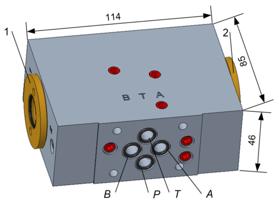
Figure 1.
General view of the valve; 1, 2—electromagnet connectors, P, T, A, B—hydraulic connectors.
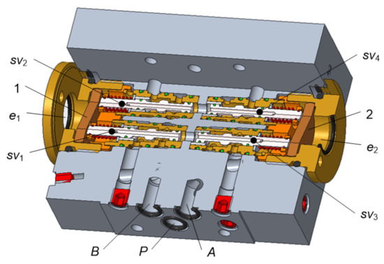
Figure 2.
Valve cross-section; 1—platen, 2—cover; —seat valve; P, A, B—hydraulic connectors.
Four two-position seat valves are installed inside the valve block. Two electromagnets are mounted on both sides using and connecting ports (Figure 1). Thus, the each electromagnet controls opening or closing of two valves simultaneously. There are standard connection ports arranged in accordance with ISO 4401 at the inlet as well as at the outlet of the valve block. The individual connectors are designated as follows: P—supply port, A, B—flow lines, T—return port. The valve is designed for a flow rate up to dm3 min−1 and a maximum operational pressure MPa. It can be used to control flow to the receiver directly or as a pilot valve.
In the default configuration, two normally opened () poppet valves denoted , and two normally closed () valves, , have been installed inside the block. The and valves have opened flow paths, when the electromagnet is not powered. Switching on the electromagnet causes pressure of the platen (1) on valve poppets, displacement of the poppets and thus closing flow. In contrast, the flow through and valves is cut-off and requires turning on power supply of electromagnet to open it by the platen (2) pressing on the poppets of and valves. The tested valve provides four positions as shown in the scheme (Figure 3).
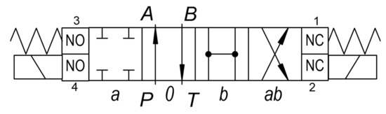
Figure 3.
Connection diagram of a configuration with two and two seat valves.
The connection ports are denoted P, A, B, T, respectively, while the state of the electromagnets is described as follows: a—only left switched , b—only right switched , 0—both unpowered, —both powered. Since the and seat valves have identical mounting dimensions, they can be used interchangeably. This allows multiple different flow way configurations to be obtained. Table 1 shows several available arrangements with different numbers of and valves used.

Table 1.
Available seat valve configurations.
Design of and seat valves is shown in Figure 4 and Figure 5, respectively. Both types consist of a body (1) in which a poppet (2) moves using the guide sleeve (3) under the force of an electromagnet and a return spring (4). The angle of the poppet head inclination is , which ensures the adequate tightness.
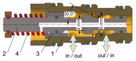
Figure 4.
type seat valve; 1—body, 2—poppet, 3—sleeve, 4—spring.
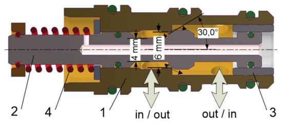
Figure 5.
type seat valve; 1—body, 2—poppet, 3—sleeve, 4—spring.
3. Flow Analysis by Means of CFD Method
The analysis includes generating fluid model which comprises all the flow paths, creating discrete models, setting up parameters and carrying out simulations.
3.1. Geometrical Fluid Model
CFD analysis requires geometrical models of the fluid. The models correspond to geometry of the individual flow paths. The paths are separated geometrically, hence the analyses can be carried out independently of each other. The path models have been created in Creo Parametric system using operations for all considered fixed positions of seat valves.
A general view of the obtained fluid models is shown in Figure 6. Based on the valve scheme (Figure 3), the following flow paths can be distinguished: , , (Figure 7), as well as and (Figure 8). Each of the , and paths contains one seat valve. In the path fluid flows through two seat valves, while in the case of the path, the flow occurs through all four seat valves in the parallel arrangement.
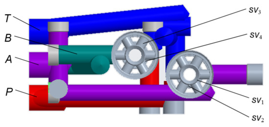
Figure 6.
Fluid model (side view); P—supply channel, A, B—flow lines, T—return channel; —seat valves.
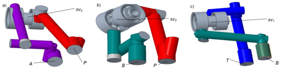
Figure 7.
Fluid models of the flow lines: (a) , (b) , (c) ; , , —seat valves.
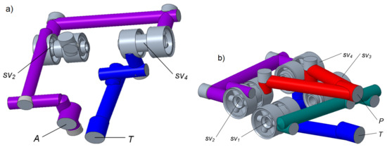
Figure 8.
Fluid models of the flow lines: (a) , (b) ; —seat valves.
3.2. Discrete Model
The each created fluid model has one inlet surface and one outlet surface. Due to the complex geometry, the models cannot be simplified using axes or planes of symmetry. Therefore, the fluid flow should be treated as three-dimensional and turbulent.
All the models were meshed in the ANSYS/Fluent system using irregular elements, including tetrahedrons in the bulk flow and three layers of prisms at the boundaries. Number of generated cells varies from 250,000 for flow path (Figure 9a) to over 2,900,000 for (Figure 9b) due to its complexity. A pressure-velocity coupling was done by the Pressure based solver with the Segregated algorithm. Mesh parameters were adjusted on the base of the previous research results and according to general recommendations provided by ANSYS/Fluent. The following quality criteria of the mesh were achieved: minimal value of the orthogonal quality , skewness between and and the maximum aspect ratio close to . The maximum allowable absolute values of both mass and momentum residuals were adopted as the convergence criteria.
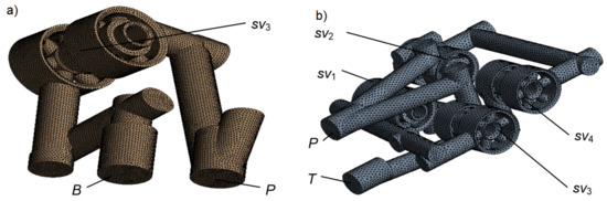
Figure 9.
Meshed models: (a) line, (b) line; —seat valves.
3.3. CFD Model Parameters
In order to carry out CFD simulation, first the kind of flow has to be determined. The Reynolds number calculated on the base of flow channel geometry, fluid viscosity and flow rate range varies from to . Hence, the turbulent flow pattern was used. ANSYS/Fluent provides a wide set of turbulence models, including , , , , and others. Based on geometrical complexity of flow channels, relatively high Reynolds number value and a general assumption that the flow is considered over the entire cross section of the channels, the model was used in the research. This model was also used in similar research on the flow through control valves [8,14,23,27].
The main model parameters, including k—kinetic energy of the turbulence and —kinetic energy dissipation factor, can be calculated based on the transport equations Equations (1) and (2). The nature of turbulence is described using Intensity I and Length scale ℓ options, Equations (3) and (4), respectively.
where is the increase in kinetic energy of turbulence, which is caused by gradient of average velocities, and represent energy generated by the buoyancy phenomenon and the compressibility of fluid, respectively, is Reynolds number and is relevant hydraulic diameter of the flow channel. The dimensionless constants were assigned using recommended values [28]: , , , , . Turbulent viscosity was calculated based on k and values:
where is fluid density. The boundary conditions were defined using physical parameters of the fluid: average velocity in the inlet channel and pressure at the outlet. The velocity magnitude was set as normal to the boundary in the Boundary Conditions/Velocity Specification Method selection box. The outlet pressure was defined as a Gauge Pressure of value MPa using the Outlet condition option. Table 2 summarizes physical parameters of the fluid and boundary conditions of the simulation model.
Table 2.
Physical parameters and boundary conditions.
3.4. Results of CFD Simulations
Calculations were made for each of the distinguished flow paths (, , , and ) with volumetric flow rate values dm3min−1. Since there are seat valves in each flow path, and the valves are characterized by similar flow resistance values, the main differences occur due to the various length and geometry of both inlet and outlet flow channels. As an example, the results obtained for and flow paths in the form of velocity and pressure distributions are shown in Figure 10 and Figure 11, respectively.
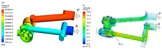
Figure 10.
Simulation results obtained with the flow path at a flow rate dm3min−1: (a) pressure distribution, (b) velocity distribution.
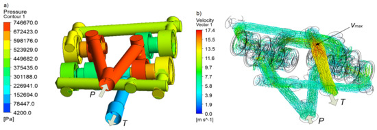
Figure 11.
Simulation results obtained with the flow path at a flow rate dm3min−1: (a) pressure distribution, (b) velocity distribution.
3.4.1. and Flow Paths
Pressure distribution on the walls of the flow path for dm3min−1 is shown in Figure 10a. The inlet pressure is near to MPa, and the highest pressure drop can be observed in the seat valve flow gaps, because of sudden step changes in cross-sectional areas of flow channels. This causes swirling and deflection of the fluid stream, as illustrated in Figure 10b, by means of velocity vectors. The maximum obtained fluid speed in the seat valve gap is m s−1.
In the case of the flow path, the result obtained for dm3min−1 is presented. In this case, despite the twice higher flow rate, the inlet pressure is less than MPa, due to the fact, that pressure drop on two seat valves connected in series is compensated by two parallel flow paths. The maximum obtained fluid speed is m s−1.
3.4.2. Determination of Flow Characteristics
The CFD analysis allowed flow resistance in all considered paths to be determined. Figure 12 shows a graph of the obtained pressure drop against flow rate. As it arises from the figure, the largest pressure drop occur in the path, which results from the largest length of flow channels and a serial flow through two seat valves. In contrast, the smallest drop occurs in the path because of a parallel flow through two pairs of seat valves.
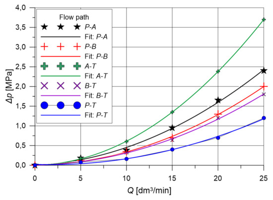
Figure 12.
Pressure drop in individual flow paths (CFD analysis).
The cross-sectional areas of the flow channels in the valve block are varied depending on the considered location. At the entrance flow area is determined by diameter of the connection port, then diameters of the channels and width of a throttling gap between the poppet and the seat valve body. The highest resistance occurs in the gap, where flow area is significantly decreased. Flow through the gap can be described by Equation (6):
With the known flow rate Q, fluid density , gap area and the determined value of discharge coefficient , a local pressure drop in the gap can be calculated. However, in the case of the considered system, apart from the seat valve itself, pressure drop also occur in the flow channels. To estimate its influence, flow simulations of a singular seat valve were carried out. Figure 13 shows pressure (a) and velocity (b) distribution obtained at a flow rate dm3 min−1, respectively. The results indicate that change in the flow direction and the division of the fluid stream may increase value of the total pressure drop significantly.
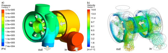
Figure 13.
Simulation results obtained for a single seat valve at a flow rate dm3min−1: (a) pressure distribution, (b) velocity distribution.
3.4.3. Discussion of Simulation Results
As part of the analysis of simulation results, pressure drop on the seat valve was compared with the one occurring in flow channels. Figure 14 shows the results obtained for considered flow paths with one seat valve: , and , respectively. As arises from the figure, the most significant flow resistance occurs on the seat valve itself, while the share of flow channels is between 5% () and 30% ().
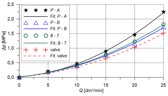
Figure 14.
Comparison of pressure drop across a seat valve to , , flow paths.
In contrast, Figure 15 presents the results obtained for and flow paths. The paths contain two seat valves connected in series. In the path, the share of flow resistance of the flow channels does not exceed 20%. On the other hand, flow resistance of the path is about 30% lower comparing to a single seat valve due to the flow through two parallel channels.
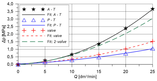
Figure 15.
Comparison of pressure drop over the flow paths containing two seat valves connected in series; and .
4. Laboratory Experiments
The results of CFD simulations were verified by means of laboratory experiments. The experiments were performed on a test bench, which was made according to the scheme shown in Figure 16. First a valve prototype was made (Figure 17a) and next the test bench was built (Figure 17b).
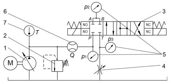
Figure 16.
Test bench scheme: 1—pump, 2—relief valve, 3—tested valve, 4—throttle valve, 5—pressure transducers, 6—flow meter, 7—temperature gauge.
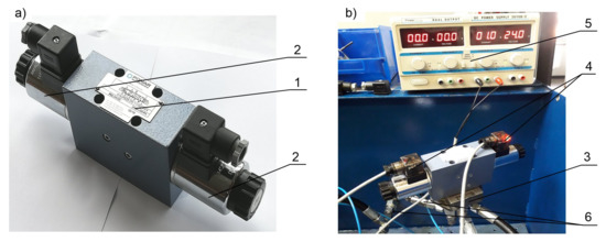
Figure 17.
Laboratory equipment; (a) valve prototype, (b) test bench; 1—valve body, 2—electromagnet, 3—mounting plate, 4—power connectors, 5—power supply, 6—pressure transducers.
The test bench contained a variable flow rate pump, a flow meter and three pressure sensors with voltage transducers. A Kracht TM flow meter with a measuring range 0.1–80 dm3 min−1 and an accuracy class % was used. Pressure sensors Trafag NAT100.0V had an accuracy class % and a range 0–10 MPa. The data was acquired using a 16-bit DAQ card at a sampling rate of 100 Hz. The measurements were carried out for identical flow rates as CFD simulations, which allowed comparison of the results to be made. Figure 18a shows comparison of flow characteristics obtained for the flow path, while Figure 18b provides the analogous graphs for the line. The summary of all the results is presented in Table 3.
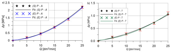
Figure 18.
Comparison of simulation and experimental results of pressure drop; (a) flow path, (b) flow path; error bars—the measurement uncertainty.
Table 3.
Comparison of simulation (S) and experimental (E) values of pressure drop MPa.
It arises from the table, that the results obtained from CFD analysis do not differ from the laboratory experiments by more than %.
5. Conclusions
The article presents results of both CFD simulations and laboratory experiments of an innovative electromagnetically controlled hydraulic control valve adapted for installation in the ISO 4401 standard. The proposed solution relies on replacing the commonly used spool with four miniature seat poppet valves, two of which are normally closed and two normally opened in the default configuration. This results in an increase in the number of operating position from three to four and provides significantly higher tightness comparing to spool valves. Simulation model was built in ANSYS environment with the turbulence model applied. Simulations were made for the volumetric flow rate in the range of 5–25 dm3min−1. The simulation results showed that the maximum pressure drop MPa occurred on the flow path at the flow rate dm3min−1. It has also been shown that the largest share in the pressure drop have seat valves, from 70% to 95% depending on the flow path. This proves that the flow channels are well profiled. Laboratory experiments were made for the same flow rate values as simulations. The each experiment consisted of setting a fixed flow rate value and measuring pressure drops at specific points of the flow paths. This allowed pressure drops to be calculated. High compliance of simulation results and experiments was obtained, the maximum difference did not exceed %. The following practical conclusions can be drawn from the research:
- the available four operating positions is of significant practical importance, especially in the context of energy saving. This is particularly important in systems where there is a need to cut off the flow in one position of an actuator and open it in the another one. In case when the actuator is locked in the working position under a pressure of MPa and the flow rate of the relieved pump is 20 dm3 min−1, the power consumption is instantaneously reduced by approximately 5 kW;
- the use of poppet seat valves ensures full tightness between the flow paths, which is difficult to achieve with spool valves. Assuming a typical operating pressure MPa, the average power consumption can be reduced by 60 W due to avoiding the leaks;
- although the proposed solution control valve contains more elements than a typical spool valve, it is characterized by simpler geometry of flow channels and includes typical two-way cartridge valves which are easy to mount or replace;
- application of CAD methods together with CFD analysis is a useful and convenient tool in the search for new design solutions of hydraulic valves as well as introducing changes in the operating characteristics.
Author Contributions
Conceptualization, E.L. and J.R.; methodology, G.F.; software, E.L.; validation, G.F. and E.L.; formal analysis, J.R.; investigation, E.L., G.F. and J.R.; resources, J.R.; writing—original draft preparation, G.F.; writing—review and editing, E.L.; visualization, G.F.; supervision, E.L.; project administration, G.F.; funding acquisition, E.L. and G.F. All authors have read and agreed to the published version of the manuscript.
Funding
This research received no external funding.
Conflicts of Interest
The authors declare no conflict of interest.
Nomenclature
| poppet gap area (m2) | |
| turbulence model constants (-) | |
| hydraulic diameter (mm) | |
| energy components of turbulence model (J) | |
| I | turbulence intensity (-) |
| specific kinetic energy of turbulence and kinetic energy dissipation (m2 s−2, m2 s−3) | |
| ℓ | turbulence length scale (mm) |
| pressure, pressure drop (MPa) | |
| Q | volumetric flow rate (dm3 min−1) |
| Reynolds number (-) | |
| Prandtl numbers (-) | |
| fluid velocity component (m s−1) | |
| fluid dynamic viscosity (Pa s) | |
| poppet gap flow coefficient (-) | |
| eddy viscosity (-) | |
| fluid density (kg m−3) |
References
- Herakovic, N.; Duhovnik, J.; Simic, M. CFD simulation of flow force reduction in hydraulic valves. Teh. Vjesn./Tech. Gaz. 2015, 22, 453–463. [Google Scholar] [CrossRef]
- Huovinen, M.; Kolehmainen, J.; Koponen, P.; Nissilä, T.; Saarenrinne, P. Experimental and numerical study of a choke valve in a turbulent flow. Flow Meas. Instrum. 2015, 45, 151–161. [Google Scholar] [CrossRef]
- Šimic, M.; Debevec, M.; Herakovič, N. Modelling of Hydraulic Spool-Valves with Specially Designed Metering Edges. Stroj. Vestn.-J. Mech. Eng. 2014, 60, 77–83. [Google Scholar] [CrossRef]
- Amirante, R.; Distaso, E.; Tamburrano, P. Sliding spool design for reducing the actuation forces in direct operated proportional directional valves: Experimental validation. Energy Convers. Manag. 2016, 119, 399–410. [Google Scholar] [CrossRef]
- Park, S. Development of a proportional poppet-type water hydraulic valve. Proc. Inst. Mech. Eng. Part C J. Mech. Eng. Sci. 2009, 223, 2099–2107. [Google Scholar] [CrossRef]
- Lisowski, E.; Filo, G. CFD analysis of the characteristics of a proportional flow control valve with an innovative opening shape. Energy Convers. Manag. 2016, 123, 15–28. [Google Scholar] [CrossRef]
- Woldemariam, E.T.; Lemu, H.G.; Wang, G.G. CFD-Driven Valve Shape Optimization for Performance Improvement of a Micro Cross-Flow Turbine. Energies 2018, 11, 248. [Google Scholar] [CrossRef]
- Gomez, I.; Gonzalez-Mancera, A.; Newell, B.; Garcia-Bravo, J. Analysis of the Design of a Poppet Valve by Transitory Simulation. Energies 2019, 12. [Google Scholar] [CrossRef]
- Zhou, J.; Hu, J.; Jing, C. Lumped Parameter Modelling of Cavitating Orifice Flow in Hydraulic Systems. Stroj. Vestn.-J. Mech. Eng. 2016, 62, 373–380. [Google Scholar] [CrossRef]
- Pan, X.; Wang, G.; Lu, Z. Flow field simulation and a flow model of servo-valve spool valve orifice. Energy Convers. Manag. 2011, 52, 3249–3256. [Google Scholar] [CrossRef]
- Sapra, M.; Bajaj, M.; Kundu, S.; Sharma, B. Experimental and CFD investigation of 100 mm size cone flow elements. Flow Meas. Instrum. 2011, 22, 469–474. [Google Scholar] [CrossRef]
- Ferreira, J.P.B.; Martins, N.M.; Covas, D.I. Ball Valve Behavior under Steady and Unsteady Conditions. J. Hydraul. Eng. 2018, 144, 04018005. [Google Scholar] [CrossRef]
- Brunone, B.; Morelli, R. Automatic control valve-induced transients in an operative pipe system. J. Hydraul. Eng. 1999, 125, 534–542. [Google Scholar] [CrossRef]
- Liao, Y.; Yuan, H.; Lian, Z.; Feng, J.; Guo, Y. Research and Analysis of the Hysteresis Characteristics of a Large Flow Directional Valve. Stroj. Vestn.-J. Mech. Eng. 2015, 61, 355–364. [Google Scholar] [CrossRef]
- El-Adawy, M.; Heikal, M.R.; Aziz, A.R.; Siddiqui, M.I.; Munir, S. Characterization of the Inlet Port Flow under Steady-State Conditions Using PIV and POD. Energies 2017, 10, 1950. [Google Scholar] [CrossRef]
- Rybarczyk, D.; Sedziak, D.; Owczarek, P.; Owczarkowski, A. Modelling of electrohydraulic drive with a valve controlled by synchronous motor. Adv. Intell. Syst. Comput. 2015, 350, 215–222. [Google Scholar]
- Wos, P.; Dindorf, R. Practical parallel position-force controller for electro-hydraulic servo drive using on-line identification. Int. J. Dyn. Control 2016, 4, 52–58. [Google Scholar] [CrossRef][Green Version]
- Stump, P.M.; Keller, N.; Vacca, A. Energy Management of Low-Pressure Systems Utilizing Pump-Unloading Valve and Accumulator. Energies 2019, 12, 4423. [Google Scholar] [CrossRef]
- Dindorf, R.; Wos, P. Force and position control of the integrated electro-hydraulic servo-drive. In Proceedings of the 20th International Carpathian Control Conference (ICCC), Krakow-Wieliczka, Poland, 26–29 May 2019. [Google Scholar] [CrossRef]
- Tamburrano, P.; Plummer, A.R.; De Palma, P.; Distaso, E.; Amirante, R. A Novel Servovalve Pilot Stage Actuated by a Piezo-Electric Ring Bender (Part II): Design Model and Full Simulation. Energies 2020, 13, 2267. [Google Scholar] [CrossRef]
- Lei, L.; Desheng, Z.; Jiyun, Z. Design and Research for the Water Low-pressure Large-flow Pilot-operated Solenoid Valve. Stroj. Vestn.-J. Mech. Eng. 2014, 60, 665–674. [Google Scholar] [CrossRef]
- Jin, Z.; Hong, W.; You, T.; Su, Y.; Li, X.; Xie, F. Effect of Multi-Factor Coupling on the Movement Characteristics of the Hydraulic Variable Valve Actuation. Energies 2020, 13, 2870. [Google Scholar] [CrossRef]
- Lisowski, E.; Filo, G. Analysis of a proportional control valve flow coefficient with the usage of a CFD method. Flow Meas. Instrum. 2017, 53, 269–278. [Google Scholar] [CrossRef]
- Lisowski, E.; Filo, G.; Rajda, J. Analysis of flow forces in the initial phase of throttle gap opening in a proportional control valve. Flow Meas. Instrum. 2018, 59, 157–167. [Google Scholar] [CrossRef]
- Filo, G.; Lisowski, E.; Rajda, J. Flow analysis of a switching valve with innovative poppet head geometry by means of CFD method. Flow Meas. Instrum. 2019, 70, 101643. [Google Scholar] [CrossRef]
- ISO 4401:2005 Hydraulic Fluid Power—Four-Port Directional Control Valves—Mounting Surfaces. 2005. Available online: www.iso.org (accessed on 23 May 2020).
- Lisowski, E.; Filo, G.; Rajda, J. Pressure compensation using flow forces in a multi-section proportional directional control valve. Energy Convers. Manag. 2015, 103, 1052–1064. [Google Scholar] [CrossRef]
- ANSYS-Fluent: Users Guide, 13th ed.; ANSYS, Inc.: Canonsburg, PA, USA, 2011.


© 2020 by the authors. Licensee MDPI, Basel, Switzerland. This article is an open access article distributed under the terms and conditions of the Creative Commons Attribution (CC BY) license (http://creativecommons.org/licenses/by/4.0/).