Abstract
In this paper, different control approaches for grid-forming inverters are discussed and compared with the grid-forming properties of synchronous machines. Grid-forming inverters are able to operate AC grids with or without rotating machines. In the past, they have been successfully deployed in inverter dominated island grids or in uninterruptable power supply (UPS) systems. It is expected that with increasing shares of inverter-based electrical power generation, grid-forming inverters will also become relevant for interconnected power systems. In contrast to conventional current-controlled inverters, grid-forming inverters do not immediately follow the grid voltage. They form voltage phasors that have an inertial behavior. In consequence, they can inherently deliver momentary reserve and increase power grid resilience.
1. Introduction
The ongoing transition of power systems from conventional generation, applying mainly synchronous machines, to inverter-dominated generation is accompanied by the loss of directly grid-coupled mass inertia. As a result, the need for inertia contribution from inverter-coupled power units becomes evident. Furthermore, inverters should contribute to grid-voltage forming, which in the interconnected power systems nowadays is being performed by synchronous generators. Grid-forming inverters are available products and their applicability for island systems has been shown [1]. Unlike conventional current-controlled inverters, such grid-forming inverters form a voltage phasor that has a certain degree of autonomy but still operates synchronously to the grid voltage. With a suitable control, the inverter can also deliver momentary reserve without any delay by retarding the voltage phasor. The property of how the voltage phasor is actuated can be used as a key indicator for the grid-forming attribute of inverters.
The idea of providing inertial response with inverters in cases of frequency deviations in order to support angle stability or frequency stability in interconnected grids was published in [2]. Meanwhile, several grid-forming control concepts for inverters have been introduced. Some of them were specifically developed for island grid applications, but in future, they may also become relevant for usage in interconnected systems. This paper’s aim is to give an overview of different kinds of control schemes and to make these different approaches comparable.
In voltage source converters (VSC), the manipulated value is the switched dc-link voltage, which is realized by means of the switching pattern of the converter legs. Therefore, the converter itself is assumed to be a controlled voltage source behind a filter inductor. The control schemes discussed here are related to the short-term voltage source controlling, i.e., how the voltage source is acting immediately after an event at the point of common coupling (PCC). Additional control loops, e.g., for resonance damping, or overlaid control loops, can be added and are detached from the specific grid-forming control approach.
Firstly, a definition of the relevant terms inertia, grid-forming and grid-following inverters is given. After that, the concepts for grid-forming voltage sources are presented. The dynamic behavior of the provided voltage phasor, for both the voltage amplitude and the voltage angle are analyzed. Starting with the dynamics of synchronous machines, grid-forming control approaches with their voltage phasor dynamics are deduced. The output power or an equivalent quantity, such as current, serves as an input for the deduced dynamical transfer function.
2. Terminology
Due to the partially misleading or contradicting use of different terms in literature, some relevant terms are explained in the following.
Electrical inertia, EI, is a property of a power system classically determined by the mechanical inertia of rotating machines within a synchronous area. The mechanical inertia of a generator results electrically in the ability to smoothen frequency deviations because of the kinetic energy stored in the rotor. From a technical point of view, EI refers to the ability to react to a change in the voltage phase angle at the point of connection with an instantaneous power response, due to the retarded reaction of the generator’s voltage phasor. Power-electronic devices with suitable control algorithms (e.g. grid-forming control) can also provide EI. In general, conventionally current-controlled inverters do not provide EI.
Grid-forming inverter, GFI, denotes an inverter having a control approach with the capability to control the terminal voltage directly and to form the grid voltage purely by inverters under consideration of necessary reserve and storage capacity. Such inverters can be able to provide inherently EI. (Reference [3] was one of the first papers to introduce the term “grid-forming“, and it has been meanwhile established in academia and industry. Accordingly, it is also used in this paper. In the opinion of the authors, more suitable terms are “voltage-forming” or “grid-voltage-forming”, since they state clearly that the grid voltage is the related physical quantity which is formed)
Current-controlled inverter, CCI, or grid-following inverter, in contrast to GFI, denotes an inverter having a control approach that controls the current injection, e.g., based on terminal voltage measurement, in order to meet a given power set point. Due to the power set point determination, the inverter can operate as a grid-feeding inverter, which injects power independent of voltage or frequency deviations at the terminal. Grid-supporting inverters can be applied to adjust reactive and active power set points under voltage or frequency deviations. Conventionally, CCIs do not provide EI, even though they could rapidly adjust their power response to frequency deviations or even to frequency derivatives. Due to delays in active power set point determination after angle or frequency changes (e.g., due to frequency measurement) their active power injection is generally delayed, compared to the active power response of devices with EI capability.
3. Functional Principle of Synchronous Machines
The best-known voltage source responsible for the voltage forming and inertial behavior of today’s ac power systems is the synchronous machine. The basic concept of a synchronous machine is that a magnetized rotor induces a voltage at the three-phase stator windings due to the rotational speed. The rotor can be constructed as permanent-excited or by means of an excitation winding (externally excited). The latter is assumed here, since it allows a beneficial control action.
Mathematically, the description for the flux linkage between rotor and stator simplifies a lot, when the variables of both rotor and stator are related to a coordinate system of the same speed as the rotor. Otherwise, the equations contain inductances, which inconveniently alter with the position of the rotor [4] (pp. 87–88).
This transformation of the coordinate system was first introduced by Park [5], where the x-axis of the coordinate system was laid on the direct axis of the rotated excitation coil. In literature, it is referred to as Park transformation or direct-quadrature-zero (dq0) transformation.
Moreover, several simplifications have been proposed, especially for small-signal stability analyses, which are also applied here. References [6] (pp. 328–347) and [7] give a good overview of the different models and their effect on the accuracy. Furthermore, detailed explanation concerning backgrounds and advanced modeling of synchronous machines can be found in [4] (pp. 83–146), [8] (pp. 45–198) and [9] (pp. 469–496).
Following the model reduction procedure in [10] (pp. 52–54), first the small resistive parts in the armature are neglected. Besides, another reasonable simplification is achieved by neglecting the very high-transient behavior of the damper windings. The purpose of the damper windings is to mitigate rotor oscillations, since a deviation from the synchronous angle speed induces high currents in the damper windings. As a result, a counter torque proportional to the frequency deviation from the grid frequency occurs. This effect can be taken into account by adding a damping torque to the swing equation in relation to the slip of the machine [11] (p. 456), [9] (p. 105). Furthermore, the induced transformer voltage, which refers to current changing in the coils (e.g. dΨ/dt), is small in comparison to the rotational electromotive force (emf) and decays quickly, so that this transient effect is neglected too.
On the whole, the mathematical description is reduced to the one-axis 3rd-order model [7]. It consists of three differential Equations (1)–(3). The first is related to the dynamic electromagnetic linkage between the rotor and stator. The others describe the electromechanical effect in the form of the swing equation:
U denotes the internal voltage source of the synchronous generator. It is composed of one part related to the excitation voltage Uf and another part related to the reactive current Ir. Both effects occur with a delay of the open-circuit time constant (Td0′). The first part reflects the reference transfer behavior of the excitation voltage Uf to the synchronous generated voltage
whereas the second term belongs to the disturbance transfer function and contributes to the internal reactance [12] (p. 6):
The interpretation is, that in the first moment after a current step, only the transient reactance xd′ is active. During the process, the reactance decays to the synchronous value xd. This transition is illustrated in Figure 1.
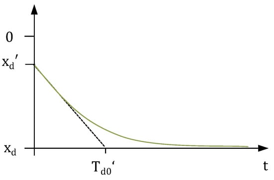
Figure 1.
Transient evolution of the impedance after a current step (derived from [13] (p. 244)).
The angle of the synchronously generated voltage U is determined by the swing Equations (2) and (3). Together with the electromagnetic Equations (1), the block diagram of the synchronous machine, shown in Figure 2, is established. In summary, it results in a voltage phasor that retardedly follows the grid voltage phasor in relation to both the amplitude (according the coil excitation time constant) and the phase angle (according to the mass inertia time constant of the rotor).
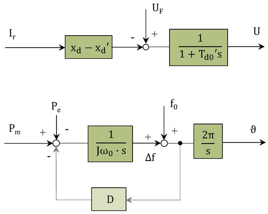
Figure 2.
Block diagram of the synchronous machine (3rd-order model).
This block representation of the synchronous machine is taken as the basis for subsequent comparisons to grid-forming inverters. Therein, Δf represents the frequency deviation from the nominal value f0 and ϑ is the rotation angle. The damping parameter D represents the mechanical damping according to friction and windage.
The equivalent circuit is depicted in Figure 3. The two circuits of the direct and quadrature axis are condensed to one complex circuit, which also serves as basis for the following elaborations. It consists of an adjusted voltage source U behind an internal inductance xi. For the whole paper, the generator convention is adopted [14] (pp. 20–27) as commonly used for power sources.
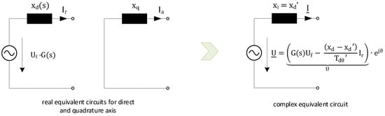
Figure 3.
Equivalent circuit of the synchronous machine.
4. Grid-Forming Inverter Control Methods
4.1. Droop-Based Grid-Forming Control Methods (e.g. Selfsync)
The idea of synchronizing parallel static inverters by means of power droops reaches back to [15] (see [16]). Following the operational principle of conventional power plants, f(P)- and U(Q)-droops with reversed relation were exploited (see Figure 4). Therein, quantities f0 and U0 denote the nominal values. In a similar way, reference [17] deals with the stand-alone operation of static inverters and suggests a method in which a voltage and frequency drop behavior in relation to the output reactive and active power is imposed. The purpose is to achieve load sharing among power sources without explicit communication. Likewise, in [18] droops are deployed in combination with a virtual flux control. In the meantime, a multitude of droop-based approaches have been published [19].
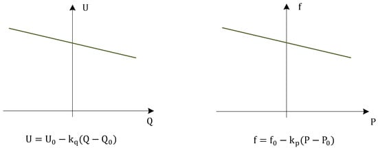
Figure 4.
Droop characteristics.
Mostly, the output power is measured and low-pass filtered with the time constant (Te, Tm), in order to eliminate oscillations, due to harmonics, and to obtain a more-smooth reaction. Afterwards, the value is fed back to generate the internal inverter voltage. A reasonable improvement compared to the normal droop control can be gained by an angle feedforward proportional to the active power flow, which was first introduced in [20] or [21] and is referenced as Selfsync. We concentrate on this approach in the following elaboration.
The related block diagram is illustrated in Figure 5. In the next step, this structure is rearranged as depicted in Figure 6. It becomes apparent that the functional principle is equivalent to that in Figure 2.
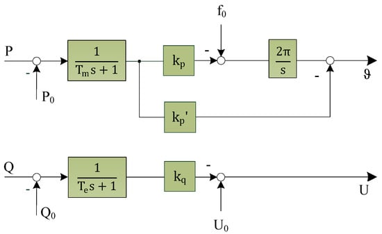
Figure 5.
Block diagram of the Selfsync control algorithm.
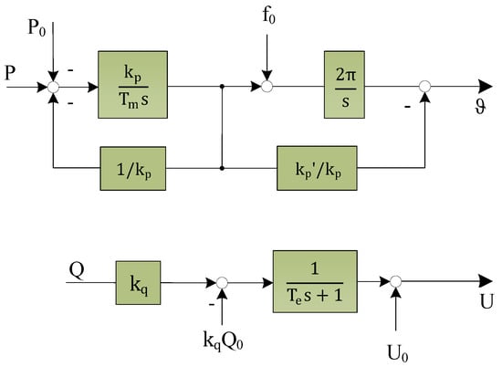
Figure 6.
Rearranged block diagram of Selfsync control algorithm.
Likewise, a reactive power value is fed back to adjust the internal voltage (electro-magnetic force), so that the droop parameter kq corresponds to (xd − xd′). Consequently, the reactive power droop can be interpreted as impedance evolution similar to that of the synchronous machine (see Figure 1): In the first moment only the filter impedance of the inverter is active and due to the imposed droop, the impedance in the reactive current path is adjusted to a higher stationary (synchronous) value. The time constant Te is in accordance to the open-circuit time constant Td0′ of the synchronous machine. It should be noted that the reactive power is used here. Strictly speaking, the relation between the reactive current and the voltage amplitude is not precisely linear here, due to voltage variations. Therefore, these conclusions are only valid around the nominal operating voltage. On the other hand, it is possible to normalize the droop parameter by the output voltage. By doing so, the reactive power droop changes to a reactive current droop.
Moreover, the active power loops also resemble each other, so that Tm/kp is equivalent to the inertia time constant and 1/kp is equal to the mechanical feedback damping parameter D. As an extension to the basic functionality, forward damping is achieved, due to the angle feedforward. This damping is much more effective against oscillation, as it bypasses the integrator. Consequently, a better stability and transient performance was observed when using such a technique. The damper windings have a similar effect, since they inherently produce a counter torque according to the slip (deviation from the synchronous rotation) of the machine.
It is noteworthy, that with synchronous machines, system parameters such as time constants and reactance are subject to the mechanical construction. At best, the feedback damping parameter D of the synchronous machine can be increased when the power system stabilizer (PSS) is designed properly [8] (pp. 766–767). In contrast, in the case of grid-forming inverters, the system parameters can be designed freely according to higher requirements.
Values typically chosen for the Selfsync control algorithm can be found in Table 1. Except for the time constants, the values are given per unit with respect to inverter nominal power and voltage. Thus, the control can easily be realized for different power ratings and voltage levels. The time constant Tm is chosen according to the acceleration time of the grid (~10 s). Hence, it is a measure for the inertia contribution in relation to the nominal power of the grid-forming unit. The time constant for the voltage amplitude is chosen lower. The droop parameters kp and kq mean that, at nominal power, the frequency or voltage drop is 5% and 10%, respectively. Additionally, an adequate feedforward damping is achieved with a value around 5 pu.

Table 1.
Exemplary parameterization of the Selfsync control algorithm.
Although only one specific droop-based method is analyzed here, other known droop-based approaches can be interpreted similarly, since the basic functional principle is the same. Nevertheless, the damping or superior control features may differ, due to some additional control loops.
In [22], an often-referenced approach concerning droop control is described. One basic element therein is the rotational matrix T. This was developed for operation in resistive grids in order to adapt the control action to the specific transfer function of the system. It means that not the measured output power values are applied to the droops but virtual values resulting from the rotations in the complex plane according to the R/X ratio of the power line. As a result, an increase in the effectiveness of the droops is achieved. However, this has a negative effect on the load sharing, since the droops control only the virtual values not the real power values. Moreover, the consistency with the conventional power system is lost, since the analogy to the synchronous machine is partially reversed. Therefore, it is not recommendable for practical applications in the main grid.
Other authors supplement the droops by differentiators for the purpose of improved transient response [23,24]
When looking at Equation (6), it becomes clear that the effect of kp,d is similar to the angle feedforward by kp′. The effect of kq,d is that the reactance of the reactive current path is virtually further increased in relation to the rate of current change during a transient process. The consequence is that the time development of the reactance is not so smooth and more dynamic.
Other approaches combine the droop control with virtual impedance loops to improve load sharing or droop operation [25,26]. Therefore, the underlying impedance parameters may differ, due to the fast-acting additional loops, but the essential control structure is retained.
4.2. Power Synchronization Loop
A further technique to realize a grid-forming control is the so-called power synchronization control depicted in Figure 7 [27]. Additional insights can be found in [28]. Other authors improved this approach by orienting closer towards the synchronization mechanism of the swing equation and include a further transfer function in order to match the dynamic order with an appropriate damping capability [29].
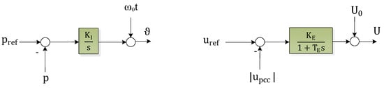
Figure 7.
Power synchronization control loop according to [27].
With regard to the angle regulation, a strong similarity to the droop-based approaches becomes obvious, because it also consists of a direct P/f-droop-characteristic. The power measurement filter and an angle feedforward are not mentioned, so that the appropriate parameters are assumed to be zero.
The voltage amplitude regulation consists of a cascade of a proportional voltage controller and optionally of a superior reactive power controller. Due to the proportional voltage controller there is also a “droop” characteristic [27], but in the opposite direction. The drooping action stems from the fact that the amplitude at the PCC is almost a linear function of the reactive current. For a better understanding, refer to the phasor diagram in Figure 8.
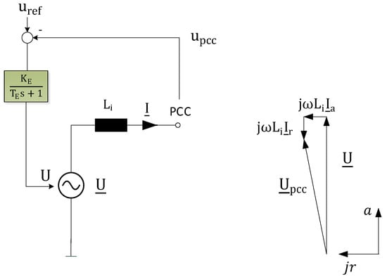
Figure 8.
Schematic voltage control in the power synchronization control loop.
It can be seen that the voltage component on the horizontal r-axis only has a negligible impact on the total amplitude. The main effect on the amplitude is brought about by the a-axis voltage drop, which results from the reactive current. Consequently, the feedback loop for regulating the amplitude corresponds to an impedance reduction, opposite to that of a Q/U-droop. The parameter KE defines the negative gain for the impedance Li, so that in a steady state, the new value is (ωLi/(1+KE)) and TE is responsible for the continuous time delay with which the impedance is adapted. This can be deduced from the transfer function from the resulting current flow to the provided voltage drop. The closed voltage amplitude loop can therefore be restated (Figure 9) under the assumption that Ia has only a very small influence on the voltage amplitude at the point of common coupling.
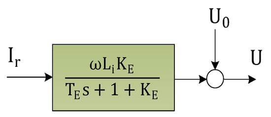
Figure 9.
Restated voltage–amplitude control loop.
4.3. Voltage Controlled Inverter (VCI)
This approach to control grid-forming inverters was published in [30]. The concept will be explained with the resulting dynamics of the voltage angle and amplitude. For the frequency control loop, the following control structure shown in Figure 10, was considered. The controller itself consists of a PI-controller and can be optionally extended by a primary control loop as it is realized by frequency droops. A transformation of the control algorithm can be found in Figure 11.
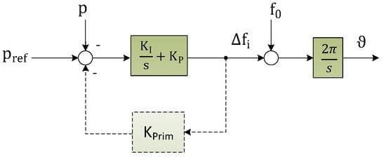
Figure 10.
Frequency controller of the voltage controlled inverter VCI according to [30].
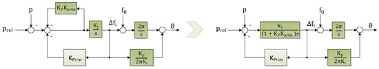
Figure 11.
Transformation of the VCI control structure.
This transformation yields the same structure for the frequency loop as in Figure 6. In addition to the swing equation, it also includes the feedforward damping (realized by Kp/2πKi) equally to that of the Selfsync approach. Here, KPrim equals the feedback damping factor D and (1+KPKPrim)/KI is the inertia time constant.
The voltage–amplitude regulation loop is shown below. With the voltage control mode, the dynamical regulation of the voltage amplitude again is deduced by following the procedure revealed in the power synchronization control (see Figure 8).
Based on the assumption that only the reactive current component has a considerable effect on the voltage amplitude, a transfer function from the reactive current to the voltage amplitude is set up (Figure 12). The effect of the PI controller results in an impedance reduction according to the principle in Figure 13. Due to the integrator, the effect of the internal reactance in the reactive current path is completely reduced to zero during the control action. In contrast to the synchronous machine (compare Figure 1), it means that the inner impedance is not increased during the transient time, but eliminated.
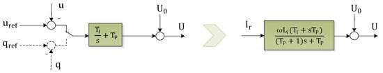
Figure 12.
Voltage control loop of the VCI.
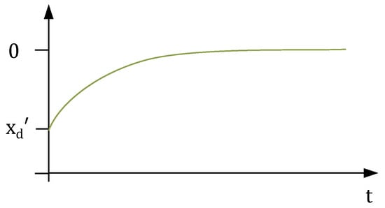
Figure 13.
Elimination of the impedance by the integrator action with the appropriate time constant.
Basically, it can be stated that a voltage controller of the terminal voltage eliminates the internal impedance within the time constant of the PI-controller, whereas a reactive power controller corresponds to an increase of the reactance value in the reactive current path.
4.4. Virtual Synchronous Machine (VSM)
Directly emulating the synchronous machine is a straightforward approach to impart grid-forming capabilities to inverters. Multiple control algorithms have been proposed [31,32,33], which carry this approach in their name. They differ in the depth of emulation and amount of additional current and voltage control, but they all include some form of the swing Equation (2). Reference [34] gives an overview of some of the published approaches and proves the equivalence of VSM and droop control with regards to small signal stability [35].
Starting with [36], the concept of a virtual synchronous machine called VISMA was applied. In this early implementation, the inverter control imposes an exact current response according to a synchronous machine model of seventh order. The output voltage is used to feed the machine model and calculate the current response in real time. By means of a hysteresis comparator, a fast adjustment of the current is achieved. In [37] the machine model was simplified for the purpose of robustness and stability and the suitability of island operation was shown.
Another well-known virtual synchronous machine concept is referenced as synchronverter [33]. The idea is again to implement the synchronous machine behavior in inverters. The control law implemented on the inverter is composed of the dynamic swing equation and algebraic equations for coupling the virtual rotor and stator side. In this, the damping of the virtual mass inertia is solely performed by feedback of the difference between VSM and reference frequency. Thus, it incorporates a frequency-power droop in terms of frequency containment reserve (previously referred to as “primary control reserve”) [38] and cannot be designed freely. In a further development [39], an additional loop is exploited from the virtual flux to the active power in order to improve the damping and a defined dynamic response.
Another detailed realization of a virtual synchronous machine can be found in [40]. Here, the swing equation is supplemented by a frequency droop. In addition, a more appropriate damping is performed by a feedback of the difference between the grid and the VSM frequency. Since the grid frequency is provided by a phase locked loop (PLL), it suffers from a minor delay. For interested readers, several subsidiary controls were added in that paper, e.g., current control or virtual impedance. However, they are more related to high-transient electromagnetic effects or internal impedance correction, both of which are not the focus of this paper.
Since all VSM concepts utilize the swing equation, the damping of the virtual mass inertia is an important criterion. A compilation of different damping strategies for virtual synchronous machines is given in [38].
As an illustrative example for VSM control methods, the VSM structure applied in [32] is derived in this paragraph. Firstly, the swing Equation (2) is expanded by damping power
which accounts for mechanical loss due to friction and windage (as in [9] (pp. 125–129)). This gives:
which is also shown in Figure 2. The damping coefficient D is a property of the physical construction of the synchronous machine and thus fixed. In VSM control, this parameter can be chosen freely. As it directly correlates active power P and frequency f, it is used to define the slope of the P(f)-characteristic of the VSM. It is renamed Kpf in order to reflect that change.
In the next step, J, ω0 and 2π are condensed into a single time constant Ta = 2H and a forward damping constant Kdf is introduced, which can be dimensioned to effectively dampen oscillations between generators.
In the Q-Branch, Ku is chosen as the slope of the Q(U)-characteristic and Tu as the excitation time constant. The resulting diagram of the control scheme is shown in Figure 14. It is quite similar to the rearranged Selfsync control shown in Figure 6.
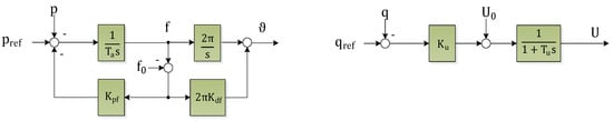
Figure 14.
Virtual synchronous machine control.
4.5. Virtual Oscillator Control (VOC)
The virtual oscillator control (VOC) differs from the previously mentioned approaches, as it is not based on phasor representation. It is a sinusoidal time domain implementation that is related to the synchronization principle of coupled oscillators in complex networks [41]. The method uses a Van der Pol oscillator with a nonlinear differential equation to generate the virtual oscillator [42]. The principle is illustrated in Figure 15.
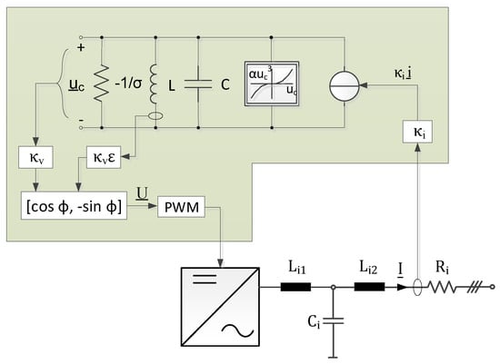
Figure 15.
Illustration of the virtual oscillator circuit according to [43].
As a feedback parameter, only the output current is applied, which is used to feed the virtual oscillator circuit. The parameters κi and κv serve as scaling factors for the interface between the real hardware and the virtual oscillator. The inductance and the capacitance of the oscillating circuit are chosen in such a way that the resonant frequency matches the nominal frequency ω0.
In [43] the dynamics of the VOC is transferred into phasor representation, which makes it comparable to phasor-based approaches. The averaged dynamics of the VCO is captured by the following equations:
with and . For this reason, a P/f- and Q/U-characteristic is achieved. Compared to the 3rd-order model of the synchronous machine (or Selfsync for example), the state variable, which is related to the mass inertia, does not exist.
For further analysis of the voltage amplitude loop, the model Formula (10) is linearized:
with the nominal voltage U0 and the nominal reactive power Q0. The block diagram of the VOC as the averaged model is shown in Figure 16. The linearized Q/U-loop reduces to a PT1 element similar to the electromagnetic behavior of the synchronous machine. In this way, 1/K corresponds to (xd − xd′) and Z/K corresponds to the time constant Td0′.
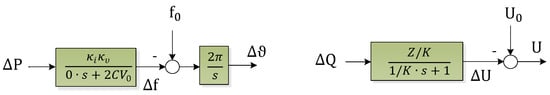
Figure 16.
Block diagram of the VOC in averaged representation.
As already mentioned above, the state variable that correlates with the frequency is not included in this method. Thus, the time constant is set to zero. The resulting P/f-control loop achieves a similar effect as it is done by the angle feedforward (feedforward damping), which is known from Selfsync or some virtual synchronous machine and voltage-controlled approaches.
However, it is important to note that the inertia time constant equals zero. As a result, an autonomous voltage phasor is formed, but it is not retarded, so it does not provide sufficient inertial support.
4.6. Matching Control
The core of matching control is the duality of the converter DC voltage and the generator angular velocity [44,45]. A good explanation of this concept is given in [46], which is taken as the basis in the following. A further, more analytical elaboration can be found in [47].
The idea of this concept is to treat the physical dc-link capacitor as storage in the same way as the moment of inertia does. For this purpose, the dc-capacitor voltage is used to adjust the frequency of the ac-converter bridge. The control law is given by [46]:
where ω is the output frequency, ωg is the nominal or grid frequency and UDC is the dc-link voltage. The control law incorporates both the dc-voltage regulation and the synchronization to the grid.
The overall functional principle is depicted in Figure 17. The control law in Equation (15) is supplemented by (U)Q-droop, in order to regulate the amplitude.
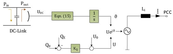
Figure 17.
Functional principle of matching control according to [46].
Together with the power equation of the dc-capacitor, a relationship between power and voltage phasor can be established (Figure 18). It describes the dynamics with which the voltage phasor is adjusted. The parameter KJ is the inertia emulation coefficient, KT is responsible for the DC-link voltage tracking and KD is the damping coefficient.

Figure 18.
Voltage phasor dynamics of matching control.
4.7. PLL-Based Modified Current-Controlled Methods
There is an ongoing discussion in the scientific community regarding the need for a phase locked loop (PLL) in grid-forming inverter types. Typically, grid-following inverters are associated with a phase locked loop [48], whereas grid-forming control methods are assumed not to apply a PLL [45], [49] or to apply it only for initial grid synchronization [27]. Another reference proposes an improved grid-forming control approach by using frequency and angle measurements through a PLL [50]. For parallel operation, all grid-forming units should incorporate some kind of synchronization mechanism. The use of a PLL is therefore not necessarily a criterion against the grid-forming capability. Even more, recent research showed that a power grid can be operated solely with an inverter using an enhanced current-controlled control scheme [51]. Thus, we cannot say generally that grid-forming units do not apply a PLL. This section will further analyze these aspects. It introduces the main concept of using a PLL in order to provide an inherent inertial response with current-controlled inverters and reports other approaches that make use of this concept.
The VSYNC project aimed to enable power system stability enhancement through inverters in combination with short-term energy storage, providing an inertial-like active power response [3,52,53]. There, a grid-following control algorithm was equipped with a suitably parameterized PLL in order to calculate an additional power set point for the inverter in analogy to a combination of the swing Equation (2) in normalized notation and the transmission Equation (16). With Pe being the electrical power between two voltage sources with amplitude U,E and angle ϑ1,2 over the inductive impedance Xi
the combination of both equations results in:
With the PLL structure shown in Figure 19, while neglecting Kp and assuming the mechanical power Pm in Equation (17) to be zero, the similarity of the PLL structure and Equation (17) becomes visible:
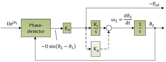
Figure 19.
Phase locked loop (PLL) structure for calculation of an additional active power setpoint for inertial response of inverters according to [53].
By choosing the PLL parameters Ki, Kd to
the PLL describes the same transient behavior as the mechanical part of a synchronous machine, which is connected to a transmission line. The derivative of the frequency as inherent output of the PLL without explicit differentiation is used as an additional active power setpoint in order to provide an inertial response [53].
The difference to other df/dt-based inertial response controllers is the calculation of the frequency derivative. Here, the frequency derivative is automatically determined within a PLL. Other approaches on the basis of current-controlled control algorithms [54,55], measure the frequency with a PLL, filter this measurement value with a low-pass, and formulate the derivative as, e.g., a multiplication with the Laplace operator s. The latter approach is therefore delayed, compared to the direct PLL-based method. Hence, the relationship between frequency derivative and power injection of df/dt-based inertial response controllers does not initially follow the swing equation.
In [56] a similar PLL-based method has been recently introduced. In contrast to [3,52,53], the loop filter has been equipped with a proportional gain Kp for additional damping and to improve the frequency detection speed, see Figure 19. However, the design of the PLL gain factors follows the same approach.
Therefore, assuming fast adjustment of the given active power setpoint, the inner angle of both introduced direct PLL-based methods corresponds to the swing equation, and they behave in the same way as synchronous machines in their frequency/active power relation. As a conclusion, an active power/frequency relation can be deduced (see Figure 20), similar to synchronous machines or grid-forming inverters.
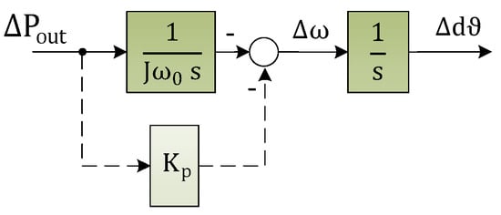
Figure 20.
Generalized transfer function between active power and voltage angle of PLL-based inertial response methods.
However, similar to the synchronization torque in synchronous machines, the synchronization principle of the PLL with its inherent relationship between power and angle can be used in a more suitable sense. Assuming the provided voltage phasor is generated using the information (especially the angle) from the PLL in the form of a voltage feedforward, by tuning the parameters of the PLL, the dynamics of the provided voltage phasor can be chosen. As a result, a retarded following voltage phasor can be created according to the slowness of the PLL. In inductive coupled grids, the way the PLL-parameters work, can be derived again from Figure 20.
This relationship is implicitly exploited in modified current-controlled approaches, e.g., [57,58,59,60]. There, the inner PI current control loop has been additionally reduced to a proportional control. Otherwise, the integrator will eliminate the retarded adjustment of the provided voltage phasor. In general, the remaining proportional current controller acts as an additional resistive impedance in series and is comparable to the concept of a virtual impedance. It introduces a further damping against electro-magnetic resonances.
Furthermore, the amplitude of the voltage feedforward is delayed in [60]. The quadrature-component of terminal voltage is omitted, because the provided voltage phasor is completely projected to the direct axis, which in turn is adjusted smoothly according to the PLL. Hence, a relationship between reactive current and voltage amplitude can be derived, which describes the impedance evolution in time as for example seen in the synchronous machine. The following considerations are in close correspondence to Figure 8.
Under consideration of a small angle difference ϑ, the circuit equation yields for the (reactive) current through the impedance Xi:
assuming UPCC being the measured terminal voltage amplitude and U being the inverters voltage amplitude.
According to the delayed (PT1) feedforward of the measured voltage, the provided voltage amplitude is a function of UPCC. In turn, the changes in the amplitude of UPCC are determined by the reactive current flow, as seen in Figure 8.
As a result, the amplitude of the internal provided voltage of the inverter can be formulated in relation to the reactive current flow:
In the Laplace domain, the initial state is not included, so that only the reaction after an impulse is described. In addition, the initial voltage is taken into account here by U0, which equals UPCC in idle mode or could be adjusted in terms of outer control loops. Consequently, the provided voltage amplitude is given as a function of the reactive current deviation ΔIr from the nominal or initial value:
The resulting block diagram (Figure 21) can be drawn from Equation (22). The interpretation is that the impedance grows in time after an evoked reactive current step. The increase of the provided voltage amplitude counteracts the cause for the current flow, so that in the closed loop, a negative feedback is achieved. As a result, the inverter is led back to the operating point before the incident.
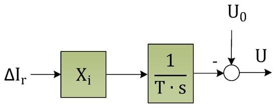
Figure 21.
Generalized transfer function between reactive power and voltage amplitude of inverters with modified grid current control.
In combination with a PLL, which might be used according to the aforementioned relationship (Figure 20), the modified current-controlled approaches in [57,58,59,60] can provide inertia and could also control a grid without the existence of other grid-forming units. For substantial inertia contribution, the PLL must be slowed down in order to cause a retarded response of the provided voltage phasor. The reduction of the classical PI-control structure to a proportional control is a plausible adjustment in order to soften the effect of the current control in favor of a slowly-following voltage feedforward. The remaining proportional controller can be regarded as an increase in the available resistive coupling impedance.
For further frequency support in [57,58,59] outer control loops have been implemented in order to adjust active power set-points dependent on frequency deviation and frequency derivative. In such case [51] demonstrates that even operating in stand-alone mode could be achieved. Therefore, inverters with enhanced current-controlled approaches with PLL for frequency and angle detection are capable of acting as grid-forming inverters. Further research on the performance is necessary.
4.8. Direct Power Control (DPC)
Another approach to be discussed is the so-called direct power control (DPC). It has in common with many other approaches the fact that the output power flow is measured to adjust the internal power-source voltage phasor. This idea of controlling the inverter’s output power directly, without a dedicated current controller and PLL reaches back to [61]. In this approach, the switching pattern of the three-phase bridge, producing the internal voltage phasor, is gained from the hysteresis comparators and the position of the estimated output voltage. The optimal switching table can be found in [61]. The hysteresis controller leads to a variable switching frequency, which may cause challenges in designing the output filter.
Although, a dedicated PLL is not used, the estimation of the output voltage gives the reference for the phase angle. As a result, the standard DPC can be categorized as a grid-following method [62].
Based on this concept, [63] uses a virtual flux similar to [18] by integrating the voltage in order to obtain the phase angle information. Due to the low-pass behavior of the integrator, a smooth and retarded reaction to voltage disturbances is achieved [64]. This effect is comparable to that of a slowly following PLL as described in Section 4.7. Moreover, in [64] this concept is developed further to DPC with a rotating-frame PI controller and space vector modulation. By doing this, the drawback caused by variable switching frequency is eliminated.
Recently, a grid-voltage modulated direct power control (GVM-DPC) was suggested [65,66]. In contrast to the approach in [64], the output voltage is directly used to apply a kind of inverse park transform and gain the vector position [67]. Consequently, the tracking performance is improved, since the delay of a PLL no longer prevails. However, the downside thereof is losing the beneficial behavior of a well-designed PLL, e.g., filtering of harmonic perturbation or inertia provision as discussed in Section 4.7. For weak grids, it was proposed to use a band-pass voltage filter for harmonic stability improvement, which in turn produces again a delay for the vector positioning [68]. Furthermore, reference [65] demonstrates the performance of the GVM-DPC after a sudden frequency variation. The result is that even transiently no power deviation occurred. Hence, the inverter perfectly follows the grid voltage angle to attain its operation point. In other words, without any retarded voltage vector positioning, this technique acts as a grid-following inverter.
Another approach that is referenced as direct power control can be found in [69]. The control scheme is given in Figure 22. There are two loops, i.e., the reactive power loop to control the voltage amplitude and the active power loop to control the angle. The voltage amplitude does not follow fast variations. After a sudden change on the grid-side, it retains its value. According to the time constant T of the integrator, the previous operating point is slowly adjusted.
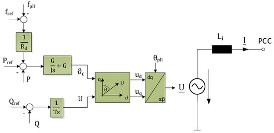
Figure 22.
Direct power control according to [69].
It should be noted that the angle ϑc is the phase angle shift related to the PLL angle θpll. Hence, a retarded adjustment of the controlled angle ϑc is undermined, when the PLL follows the grid voltage too quickly. Thus, for analyzing the overall control performance, the dynamics of the PLL is of great importance. A closer look into the PLL and its parameterization is not given in the Reference.
However, if the PLL is designed in the aforementioned manner (see Section 4.7), an inherent reaction with active power injection is given, because of the retarded following of the grid angle. With some time delay, the PI controller behind adjusts the former operating point, due to the integral part of the controller. The proportional part serves as a type of feedforward control. With a well-designed PLL for the purpose of a damped inertia contribution, the proportional part could be neglected. The authors would like to emphasize that this method does not generally have a grid-forming capability. However, with a well-designed PLL, damped inertia contribution and even a stand-alone operation could be realized.
5. Conclusions and Outlook
Both, synchronous machines and suitably controlled static converters with sufficient energy reserves can autonomously form the grid voltage and provide electrical inertia. Grid-forming inverters which incorporate electrical inertia can be realized with different control methods. Several approaches have been reviewed and the dynamic behavior of the provided voltage phasor was analyzed for both voltage amplitude and voltage angle. In most cases, the dynamic behavior was described in the form of a transfer block diagram from the active and reactive power (or current) to the provided voltage angle and amplitude, respectively. In that way, an illustrative representation in terms of the dynamic order or damping capability was given.
The retardedly following voltage angle is a key property of grid-forming inverters. In predominately inductive grids, such inverters inherently provide electrical inertia. The contribution to momentary reserve can be defined directly through the retarded reaction of the voltage phasor. All mentioned methods could form a retardedly following voltage angle, except for the virtual oscillator circuit and fast phase-locked-loops (PLL). Additionally, most of them leverage a feedforward damping in any case, which is equally as effective as the damper windings in synchronous machines, but with the notable difference that these parameters are not restricted to physical construction limits. Free from these physical restrictions, electrical power systems could be more freely designed concerning their time constants and damping performance.
The voltage amplitude branch is more difficult to deduce and analyze, since two opposite operational modes have to be considered: the reactive control and the voltage amplitude control at the point of common coupling. In case of the droop control, a reactive power value is used as feedback. Thus, the derivation of a dynamic transfer function from the reactive power to the amplitude of the voltage phasor is straightforward. In contrast, in approaches with a feedback of a voltage value, an analogy is not obvious. This was solved using the assumption that in inductive networks, the voltage amplitude deviation at the terminals is a function of the reactive current flow, so that again a relation between reactive current or power and the provided voltage amplitude is established. Voltage droop control has the aim of defining the reactance for the reactive current component in order to increase the reactive power sharing. In case of weak grids or in case of electrically distant power sources, the control of the voltage amplitude at the point of common coupling is reasonable, so that both modes have their application. Depending on the grid situation, either one or the other mode is preferable. In all cases, the control action can be interpreted as an impedance evolution in time after a reactive current step, either in a positive or in a negative direction. This was illustrated here in the form of a dynamic transfer function from reactive current to the amplitude of the internally provided voltage phasor.
Author Contributions
Conceptualization, P.U., M.N. and P.S.; methodology, P.U. and M.N.; formal analysis, P.U., M.N. and F.W.; writing—original draft preparation, P.U., M.N. and F.W.; writing—review and editing, P.S., M.N. and P.U.; visualization, P.U., M.U. and F.W.; supervision, P.S.; project administration, P.S.; funding acquisition, P.S. All authors agree to the published version of the manuscript.
Funding
We acknowledge the support of our work by the German Ministry for Economic Affairs and Energy and the Projekträger Jülich within the project “Control and Stability in Inverter Dominated Interconnected Systems-Grid Control 2.0” (FKZ 0350023A). Only the authors are responsible for the content of this publication. This paper does not necessarily reflect the consolidated opinion of the project consortium “Netzregelung 2.0”. The founding sponsor had no role in the design of the study; in the collection, analyses, or interpretation of data; in the writing of the manuscript, and in the decision to publish the results.
Conflicts of Interest
The employer (non-profit research institute) of the authors is patent holder of one of the listed grid-forming control approaches (Selfsync). The patent expires in August 2021.
References
- Engler, A.; Hardt, C.; Strauss, P.; Vandenbergh, M. Parallel Operation of Generators for Stand-Alone Single-Phase Hybrid Systems—First Implementation of a new control Technology. In Proceedings of the 17th European Photovoltaic Solar Energy Conference, München, Germany, 22–26 October 2001; WIP-Renewable Energies: Munich, Germany, 2001; pp. 2690–2693. [Google Scholar]
- Visscher, K.; de Haan, S.W.H. Virtual synchronous machines (VSG’s) for frequency stabilisation in future grids with a significant share of decentralized generation. In Proceedings of the CIRED Seminar 2008: SmartGrids for Distribution, Frankfurt, Germany, 23–24 June 2008; pp. 334–337. [Google Scholar]
- Engler, A.; Haas, O.; Kansteiner, B.; Raptis, F.; Sachau, J.; Zacharias, P. Control of Parallel Working Power Units in Expandable Grids. In Proceedings of the 14th European Photovoltaic Solar Energy Conference, Barcelona, Spain, 30 June–4 July 1997; Ossenbrink, H.A., Helm, P., Ehmann, H., Eds.; H.S. Stephens & Associates: Bedfort, UK, 1997; pp. 2029–2032. [Google Scholar]
- Anderson, P.M.; Fouad, A.-A.A. Power System Control and Stability, 2nd ed.; IEEE Press, Wiley-Interscience: Piscataway, NJ, USA, 2003; ISBN 9780471238621. [Google Scholar]
- Park, R.H. Two-reaction theory of synchronous machines generalized method of analysis-part I. Trans. Am. Inst. Electr. Eng. 1929, 48, 716–727. [Google Scholar] [CrossRef]
- Milano, F. Power System Modelling and Scripting; Springer: Heidelberg, Germany, 2010; ISBN 3642136680. [Google Scholar]
- Weckesser, T.; Johannsson, H.; Ostergaard, J. Impact of model detail of synchronous machines on real-time transient stability assessment. In Proceedings of the 2013 IREP Symposium Bulk Power System Dynamics and Control—IX Optimization, Security and Control of Emerging Power Grid (IREP), Rethymnon, Crete, Greece, 25–30 August 2013; Voumas, C., Ed.; IEEE: Piscataway, NJ, USA, 2013. [Google Scholar]
- Prabha, K. Power System Stability and Control, 1st ed.; McGraw-Hill: Hightstown, NJ, USA, 1994. [Google Scholar]
- Machowski, J.; Lubosny, Z.; Bialek, J.W.; Bumby, J.R. Power System Dynamics: Stability and Control, 3rd ed.; John Wiley: Hoboken, NJ, USA, 2020; ISBN 9781119526346. [Google Scholar]
- Van Cutsem, T.; Βουρνάς, Κ. Voltage Stability of Electric Power Systems, 1st ed.; Springer Science + Business Media: Dordrecht, The Netherlands, 1998; ISBN 9780792381396. [Google Scholar]
- Sauer, P.W.; Pai, M.A. Power System Dynamics and Stability, updated ed.; Stipes Publishing L.L.C: Champaign, IL, USA, 2006; ISBN 9781588746733. [Google Scholar]
- Crastan, V.; Westermann, D. Elektrische Energieversorgung 3. Dynamik, Regelung und Stabilität, Versorgungsqualität, Netzplanung, Betriebsplanung und -Führung, Leit- und Informationstechnik, FACTS, HGÜ, 3rd ed.; Springer: Berlin/Heidelberg, Germany, 2012; ISBN 3642201008. [Google Scholar]
- Crastan, V. Elektrische Energieversorgung 1. Netzelemente, Modellierung, Stationäres Verhalten, Bemessung, Schalt- und Schutztechnik, 3rd ed.; Springer: Berlin/Heidelberg, Germany, 2015; ISBN 366245985X. [Google Scholar]
- Oeding, D.; Oswald, B.R. Elektrische Kraftwerke und Netze, 7th ed.; Springer: Heidelberg, Germany, 2011; ISBN 3642192459. [Google Scholar]
- Alberto, A. Arrangement of Parallel Static AC Power Sources Proportions. U.S. Patent 3864620A, 11 September 1973. [Google Scholar]
- Torres, L.A.B.; Hespanha, J.P.; Moehlis, J. Power supply synchronization without communication. In Proceedings of the 2012 IEEE Power & Energy Society General Meeting, San Diego, CA, USA, 22–26 July 2012. [Google Scholar]
- Kawabata, T.; Higashino, S. Parallel operation of voltage source inverters. IEEE Trans. Ind. Appl. 1988, 24, 281–287. [Google Scholar] [CrossRef]
- Chandorkar, M.C.; Divan, D.M.; Adapa, R. Control of parallel connected inverters in standalone AC supply systems. IEEE Trans. Ind. Appl. 1993, 29, 136–143. [Google Scholar] [CrossRef]
- Tayab, U.B.; Roslan, M.A.B.; Hwai, L.J.; Kashif, M. A review of droop control techniques for microgrid. Renew. Sustain. Energy Rev. 2017, 76, 717–727. [Google Scholar] [CrossRef]
- Engler, A. Device for Parallel Operation of Equal Range Single-Phase or Three-Phase Voltage Sources. EP1286444B1, 21 August 2001. [Google Scholar]
- Engler, A. Regelung von Batteriestromrichtern in Modularen und Erweiterbaren Inselnetzen. Ph.D. Thesis, Universität Kassel, Kassel, Germany, 2002. [Google Scholar]
- De Brabandere, K.; Bolsens, B.; van den Keybus, J.; Woyte, A.; Driesen, J.; Belmans, R. A voltage and frequency droop control method for parallel inverters. IEEE Trans. Power Electron. 2007, 22, 1107–1115. [Google Scholar] [CrossRef]
- Yajuan, G.; Weiyang, W.; Xiaoqiang, G.; Herong, G. An improved droop controller for grid-connected voltage source inverter in microgrid. In Proceedings of the 2nd IEEE International Symposium on Power Electronics for Distributed Generation Systems (PEDG), Hefei, China, 16–18 June 2010; IEEE: Piscataway, NJ, USA, 2010; pp. 823–828. [Google Scholar]
- Guerrero, J.M.; GarciadeVicuna, L.; Matas, J.; Castilla, M.; Miret, J. A wireless controller to enhance dynamic performance of parallel inverters in distributed generation systems. IEEE Trans. Power Electron. 2004, 19, 1205–1213. [Google Scholar] [CrossRef]
- Yao, W.; Chen, M.; Matas, J.; Guerrero, J.M.; Qian, Z.-M. Design and analysis of the droop control method for parallel inverters considering the impact of the complex impedance on the power sharing. IEEE Trans. Ind. Electron. 2011, 58, 576–588. [Google Scholar] [CrossRef]
- Wang, X.; Blaabjerg, F.; Chen, Z. An improved design of virtual output impedance loop for droop-controlled parallel three-phase voltage source inverters. In Proceedings of the IEEE Energy Conversion Congress and Exposition (ECCE), Raleigh, NC, USA, 15–20 September 2012; IEEE: Piscataway, NJ, USA, 2012; pp. 2466–2473. [Google Scholar]
- Zhang, L.; Harnefors, L.; Nee, H.-P. Power-synchronization control of grid-connected voltage-source converters. IEEE Trans. Power Syst. 2010, 25, 809–820. [Google Scholar] [CrossRef]
- Zhang, L. Modeling and Control of VSC-HVDC Links Connected to Weak AC Systems. Ph.D. Thesis, KTH Royal Institute of Technology, Stockholm, Sweden, 2010. [Google Scholar]
- Remon, D.; Cantarellas, A.M.; Rakhshani, E.; Candela, I.; Rodriguez, P. An active power synchronization control loop for grid-connected converters. In Proceedings of the IEEE Power & Energy Society General Meeting, National Harbor, MD, USA, 27–31 July 2014; IEEE: Piscataway, NJ, USA, 2014. [Google Scholar]
- Laudahn, S.; Seidel, J.; Engel, B.; Bulo, T.; Premm, D. Substitution of synchronous generator based instantaneous frequency control utilizing inverter-coupled DER. In Proceedings of the 7th International Symposium on Power Electronics for Distributed Generation Systems (PEDG), Vancouver, BC, Canada, 27–30 June 2016; IEEE: Piscataway, NJ, USA, 2016. [Google Scholar]
- Hesse, R.; Turschner, D.; Beck, H.-P. Micro grid stabilization using the Virtual Synchronous Machine (VISMA). In Proceedings of the International Conference on Renewable Energies and Power, Valencia, Spain, 15–17 April 2009. [Google Scholar]
- Glockler, C.; Duckwitz, D.; Welck, F. Virtual synchronous machine control with virtual resistor for enhanced short circuit capability. In Proceedings of the 2017 IEEE PES Innovative Smart Grid Technologies Conference Europe (ISGT-Europe), Torino, Italy, 26–29 September 2017; IEEE: Piscataway, NJ, USA, 2017. [Google Scholar]
- Zhong, Q.-C.; Weiss, G. Synchronverters: Inverters That Mimic Synchronous Generators. IEEE Trans. Ind. Electron. 2011, 58, 1259–1267. [Google Scholar] [CrossRef]
- D’Arco, S.; Suul, J.A. Virtual synchronous machines—Classification of implementations and analysis of equivalence to droop controllers for microgrids. In Proceedings of the IEEE Grenoble PowerTech, Grenoble, France, 16–20 June 2013; IEEE: Piscataway, NJ, USA, 2013. [Google Scholar]
- D’Arco, S.; Suul, J.A. Equivalence of Virtual Synchronous Machines and Frequency-Droops for Converter-Based MicroGrids. IEEE Trans. Smart Grid 2014, 5, 394–395. [Google Scholar] [CrossRef]
- Beck, H.-P.; Hesse, R. Virtual synchronous machine. In Proceedings of the 2007 9th International Conference on Electrical Power Quality and Utilisation, Barcelona, Spain, 9–11 October 2007; IEEE: Piscataway, NJ, USA, 2007; pp. 1–6. [Google Scholar]
- Chen, Y.; Hesse, R.; Turschner, D.; Beck, H.-P. Investigation of the Virtual Synchronous Machine in the island mode. In Proceedings of the 2012 3rd IEEE PES Innovative Smart Grid Technologies Europe (ISGT Europe), Berlin, Germany, 14–17 October 2012; IEEE, Ed.; IEEE: Piscataway, NJ, USA, 2012; pp. 1–6. [Google Scholar]
- Ebrahimi, M.; Khajehoddin, S.A.; Karimi-Ghartemani, M. An Improved Damping Method for Virtual Synchronous Machines. IEEE Trans. Sustain. Energy 2019, 10, 1491–1500. [Google Scholar] [CrossRef]
- Dong, S.; Chen, Y.C. Adjusting Synchronverter Dynamic Response Speed via Damping Correction Loop. IEEE Trans. Energy Convers. 2017, 32, 608–619. [Google Scholar] [CrossRef]
- D’Arco, S.; Suul, J.A.; Fosso, O.B. A Virtual Synchronous Machine implementation for distributed control of power converters in SmartGrids. Electr. Power Syst. Res. 2015, 122, 180–197. [Google Scholar] [CrossRef]
- Sinha, M.; Dorfler, F.; Johnson, B.B.; Dhople, S.V. Uncovering droop control laws embedded within the nonlinear dynamics of Van der Pol oscillators. IEEE Trans. Control Netw. Syst. 2017, 4, 347–358. [Google Scholar] [CrossRef]
- Johnson, B.B.; Sinha, M.; Ainsworth, N.G.; Dorfler, F.; Dhople, S.V. Synthesizing virtual oscillators to control islanded inverters. IEEE Trans. Power Electron. 2016, 31, 6002–6015. [Google Scholar] [CrossRef]
- Johnson, B.; Rodriguez, M.; Sinha, M.; Dhople, S. Comparison of virtual oscillator and droop control. In Proceedings of the IEEE 18th Workshop on Control and Modeling for Power Electronics (COMPEL), Stanford, CA, USA, 9–14 July 2017; IEEE: Piscataway, NJ, USA, 2017. [Google Scholar]
- Cvetkovic, I.; Boroyevich, D.; Burgos, R.; Li, C.; Mattavelli, P. Modeling and control of grid-connected voltage-source converters emulating isotropic and anisotropic synchronous machines. In Proceedings of the IEEE 16th Workshop on Control and Modeling for Power Electronics (COMPEL), Vancouver, BC, Canada, 12–15 July 2015; IEEE: Piscataway, NJ, USA, 2015. [Google Scholar]
- Milano, F.; Dorfler, F.; Hug, G.; Hill, D.J.; Verbic, G. Foundations and challenges of low-inertia systems (Invited Paper). In Proceedings of the 2018 Power Systems Computation Conference (PSCC), Dublin, Ireland, 11–15 June 2018; IEEE: Piscataway, NJ, USA, 2018. [Google Scholar]
- Huang, L.; Xin, H.; Wang, Z.; Wu, K.; Wang, H.; Hu, J.; Lu, C. A virtual synchronous control for voltage-source converters utilizing dynamics of DC-Link capacitor to realize self-synchronization. IEEE J. Emerg. Sel. Top. Power Electron. 2017, 5, 1565–1577. [Google Scholar] [CrossRef]
- Jouini, T.; Arghir, C.; Dörfler, F. Grid-friendly matching of synchronous machines by tapping into the DC storage. IFAC-PapersOnLine 2016, 49, 192–197. [Google Scholar] [CrossRef]
- Lasseter, R.; Chen, Z.; Pattabiraman, D. Grid-Forming Inverters: A Critical Asset for the Power Grid. IEEE J. Emerg. Sel. Top. Power Electron. 2020, 8, 925–935. [Google Scholar] [CrossRef]
- Mo, O.; D’Arco, S.; Suul, J.A. Evaluation of Virtual Synchronous Machines with Dynamic or Quasi-Stationary Machine Models. IEEE Trans. Ind. Electron. 2017, 64, 5952–5962. [Google Scholar] [CrossRef]
- Rokrok, E.; Qoria, T.; Bruyere, A.; Francois, B.; Guillaud, X. Effect of Using PLL-Based Grid-Forming Control on Active Power Dynamics Under Various SCR. In Proceedings of the IECON 2019—45th Annual Conference of the IEEE Industrial Electronics Society, Lisbon, Portugal, 14–17 October 2019; IEEE: Piscataway, NJ, USA, 2019; pp. 4799–4804. [Google Scholar]
- Duckwitz, D. Power System Inertia. Ph.D. Thesis, Universität Kassel, Kassel, Germany, 2019. [Google Scholar]
- Karapanos, V.; de Haan, S.; Zwetsloot, K. Real time simulation of a power system with VSG hardware in the loop. In Proceedings of the IECON 2011—37th Annual Conference of IEEE Industrial Electronics Society, Melbourne, Vic, Australia, 7–10 November 2011; IEEE: Piscataway, NJ, USA, 2011; pp. 3748–3754. [Google Scholar]
- Van Wesenbeeck, M.P.N.; de Haan, S.W.H.; Varela, P.; Visscher, K. Grid tied converter with virtual kinetic storage. In Proceedings of the IEEE Bucharest PowerTech (POWERTECH) 2009, Bucharest, Romania, 28 June–2 July 2009; IEEE: Piscataway, NJ, USA, 2009. [Google Scholar]
- Duckwitz, D. Performance of df/dt-based inertia control during emergency islanding. In Proceedings of the 15th Wind Integration Workshop, Vienna, Austria, 15–17 November 2016; Betancourt, U., Ackermann, T., Eds.; Energynautics GmbH: Darmstadt, Germany, 2016. [Google Scholar]
- Duckwitz, D.; Fischer, B. Modeling and design of df/dt -based inertia control for power converters. IEEE J. Emerg. Sel. Top. Power Electron. 2017, 5, 1553–1564. [Google Scholar] [CrossRef]
- Laudahn, S. Dynamisches Verhalten von Wechselrichterbasierten Erzeugungsanlagen im Kontext Eines Sicheren und Stabilen Netzbetriebs. Ph.D. Thesis, TU Braunschweig, Braunschweig, Germany, 2017. [Google Scholar]
- Erlich, I.; Korai, A. Study on the minimum share of conventional generation units required for stable operation of future converter-dominated grids. In Proceedings of the 2018 IEEE Power & Energy Society General Meeting (PESGM), Portland, OR, USA, 5–10 August 2018; IEEE: Piscataway, NJ, USA, 2018. [Google Scholar]
- Erlich, I.; Korai, A.; Neumann, T.; Koochack Zadeh, M.; Vogt, S.; Buchhagen, C.; Rauscher, C.; Menze, A.; Jung, J. New control of wind turbines ensuring stable and secure operation following islanding of wind farms. IEEE Trans. Energy Convers. 2017, 32, 1263–1271. [Google Scholar] [CrossRef]
- Korai, A.W.; Erlich, I. Frequency dependent voltage control by DER units to improve power system frequency stability. In Proceedings of the 2015 IEEE Eindhoven PowerTech, Eindhoven, The Netherlands, 29 June–2 July 2015; pp. 1–6. [Google Scholar]
- Winter, P.; Wrede, H. Impact of power converter control on transient stability of power systems. In Proceedings of the Conference on Sustainable Energy Supply and Energy Storage Systems, Hamburg, Germany, 20–21 September 2018; Schulz, D., Ed.; VDE Verlag GmbH: Berlin, Germany, 2018. [Google Scholar]
- Noguchi, T.; Tomiki, H.; Kondo, S.; Takahashi, I. Direct power control of PWM converter without power-source voltage sensors. IEEE Trans. Ind. Appl. 1998, 34, 473–479. [Google Scholar] [CrossRef]
- Wang, X.; Guerrero, J.M.; Blaabjerg, F.; Chen, Z. A Review of Power Electronics Based Microgrids. J. Power Electron. 2012, 12, 181–192. [Google Scholar] [CrossRef]
- Malinowski, M.; Kazmierkowski, M.P.; Hansen, S.; Blaabjerg, F.; Marques, G.D. Virtual-flux-based direct power control of three-phase PWM rectifiers. IEEE Trans. Ind. Appl. 2001, 37, 1019–1027. [Google Scholar] [CrossRef]
- Malinowski, M.; Jasinski, M.; Kazmierkowski, M.P. Simple Direct Power Control of Three-Phase PWM Rectifier Using Space-Vector Modulation (DPC-SVM). IEEE Trans. Ind. Electron. 2004, 51, 447–454. [Google Scholar] [CrossRef]
- Gui, Y.; Kim, C.; Chung, C.C.; Guerrero, J.M.; Guan, Y.; Vasquez, J.C. Improved Direct Power Control for Grid-Connected Voltage Source Converters. IEEE Trans. Ind. Electron. 2018, 65, 8041–8051. [Google Scholar] [CrossRef]
- Gui, Y.; Wang, X.; Wu, H.; Blaabjerg, F. Voltage-Modulated Direct Power Control for a Weak Grid-Connected Voltage Source Inverters. IEEE Trans. Power Electron. 2019, 34, 11383–11395. [Google Scholar] [CrossRef]
- Gui, Y.; Wang, X.; Blaabjerg, F.; Pan, D. Control of Grid-Connected Voltage-Source Converters: The Relationship Between Direct-Power Control and Vector-Current Control. IEEE Ind. Electron. Mag. 2019, 13, 31–40. [Google Scholar] [CrossRef]
- Gui, Y.; Wang, X.; Blaabjerg, F. Vector Current Control Derived from Direct Power Control for Grid-Connected Inverters. IEEE Trans. Power Electron. 2019, 34, 9224–9235. [Google Scholar] [CrossRef]
- Ndreko, M.; Rüberg, S.; Winter, W. Grid forming control for stable power systems with up to 100% inverter based generation: A paradigm scenario using the IEEE 118-Bus system. In Proceedings of the 17th Wind Integration Workshop, Stockholm, Sweden, 17–19 October 2018; Betancourt, U., Ackermann, T., Eds.; Energynautics GmbH: Darmstadt, Germany, 2018. [Google Scholar]
© 2020 by the authors. Licensee MDPI, Basel, Switzerland. This article is an open access article distributed under the terms and conditions of the Creative Commons Attribution (CC BY) license (http://creativecommons.org/licenses/by/4.0/).