1. Introduction
The security-constrained optimal power flow (SCOPF) is an essential tool for making a day-ahead and real-time generation plan [
1]. From the perspective of control measures, the SCOPF model can be divided into the preventive SCOPF (PSCOPF) model and the corrective SCOPF (CSCOPF) model. The former model is widely used in current operations of large-scale [
2] and island power systems [
3]. The operating point obtained by this model can guarantee the safe operation of systems under all credible contingencies. How to filter the contingency set determines to a great extent the performance of PSCOPF model [
4]. For given contingencies, results of the PSCOPF model are conservative with the high generation cost. The risk conception has been introduced in [
5] to enhance its economics. In [
6], an identification method of superfluous constraints has been proposed and the model of PSCOPF can be simplified and efficiently solved. With the large-scale access of sustainable energy and frequent occurrences of natural disasters, the operation environment of power systems becomes more complex and the feasible region of PSCOPF model may not exist in some difficult operating conditions.
For seeking the lower operating cost and more flexible dispatch plans, the CSCOPF model has been put forward. In this model, corrective measures such as the unit rescheduling and load shedding are utilized after the contingency occurrence to maintain the transmission security of systems [
7]. There have been some trails about using the CSCOPF model in energy management systems to help operators make timely and reasonable dispatch decisions [
8]. However, two main problems hinder its wide application. The first problem is the heavy computational burden caused by the huge number of contingencies especially for large-scale systems and coupling constraints between the preventive control and corrective control. Many efforts have been devoted to shortening the solving time. In [
9], Benders decomposition has been applied to solve the CSCOPF model, and the computational complexity has been analyzed. Results showed that the computation speed was significantly improved without sacrificing the accuracy, whether in the serial or parallel computing environment. In [
10], an iterative approach that comprises four modules has been proposed, and its performance was better than the direct approach and Benders decomposition. A hybrid method has been used to solve the CSCOPF model in [
11] where the maximum feasible region was randomly searched through evolutionary algorithms and then deterministic solutions were provided by the interior-point method. A similar solving strategy has also been adopted in [
12], and the optimal coordination of the preventive control and the corrective control was obtained.
A more significant problem of the CSCOPF model is the insecurity of power systems during the post-contingency stage. After the contingency such as line failures or generator outages, conventional corrective measures like the unit rescheduling cannot be immediately implemented due to the limit of ramping rates. The system still operates under the preventive control while violations of line power flow and bus voltages may happen. Once cascading failures are triggered, the effectiveness of pre-made corrective plan is influenced, and the scope of the original accident could be extended. Some previous work has been done to improve the security of the CSCOPF model. An optimal locating method for support generator units has been proposed in [
13] to improve ramping abilities and enhance the robustness of systems. In [
14], quick-start units have been utilized in corrective actions for reducing the duration of post-contingency stage. References [
15,
16] have discussed that the fast-response distributed battery energy storage can be used to alleviate post-contingency overloads and reduce the power flow below the short-term emergency rating. In [
17], the state of charge has been considered in the distributed energy storage model and results showed that the generation cost increased as the initial charging state declined. The post-contingency demand response has been used to relieve overflows incurred by the renewable generation fluctuation and “N−1” contingencies in [
18]. References [
19,
20] have analyzed the risk of cascading failures caused by post-contingency overloads in the alternating current (AC) and direct current (DC) power transmission network, while the thyristor controlled series capacitor and the multi-terminal direct current have been applied to minimize the load shedding and generation rescheduling, respectively. In addition, the model predictive control (MPC) provides a higher perspective beyond static and open-loop approaches. It is a class of strategies that utilize a process model to establish a control sequence for controlling the future behavior of systems over a horizon [
21]. Under this framework, the generation redispatch, load shedding, and regulating transformers have been applied to alleviate emergency thermal loads in [
22,
23]. Moreover, the energy storage and curtailment of renewables have also been identified as corrective actions in [
24].
In this paper, the DC power flow is utilized while post-contingency line overloads are the insecurity problem discussed and solved. The essence of this problem can be described as the lack of short-term transfer capacities of power grids. Compared with approaches such as using quick-start generators, distributed battery energy storage, demand response, and other power flow controllers, the method of improving line capacities could be more direct and effective. The line thermal rating provides a novel perspective instead of conventional power flow limits. The static power flow rating obtained under the worst environment condition is usually conservative. Reference [
25] has provided a report of two pioneering schemes in the U.S. and the U.K. where the real-time thermal rating was applied. A new power flow formulation considered the line electro-thermal coupling effect has been introduced in [
26], and the error in power transfer evaluation decreased by about 20% by using this method. In [
27,
28,
29], the thermal rating of transmission lines has been utilized to increase the threshold value of wind power integration and avoid the unnecessary tripping of pre-selected generation assets. Besides the static rating difference, transmission lines have the thermal inertia and corresponding time constants range between several mins and ten mins [
30]. This means that dynamic variations of conductor temperatures cannot be ignored especially for the short-term post-contingency stage discussed in this paper. Reference [
31] has demonstrated that the neglect of transient thermal behaviors of lines caused the underestimation of power transfer capabilities and led to misoperations. In [
32,
33], the concept of electrothermal coordination has been proposed and the numerical analysis through a number of case studies validated its benefits in augmenting power transfer capability, emergency control, congestion management, and improving the system loadability. A temperature dependent power flow model has been established in [
34] where the dependence of line resistances on conductor temperature was taken into account. In [
35], the dynamic electrothermal effect has been brought into safety constraints of the post-contingency power flow control to excavate the overload endurance capability of lines.
When the dynamic thermal process of lines is considered in optimal power flow models, the heat balance equation (HBE) which describes variations of conductor temperatures must be integrated. Because the radiated heat loss rate is proportional to the fourth power of the conductor temperature, the HBE is a nonlinear differential equation. How to solve those electrothermal coupling optimization problems becomes a challenge. In [
32,
33], a modified Euler method has been used to discretize the HBE and then the problem was broken down into several linearized subproblems whose solutions were iteratively refined and linked. An approximate quadratic relationship between the temperature and the square of current has been derived by some reasonable approximations in [
34], and the analytical solution of HBE was obtained for a step change in currents. Reference [
35] has proposed that, through transforming the HBE into algebraic difference equations by a numerical integration method, the optimal solution can be realized by combining those transformed equations with other algebraic equations.
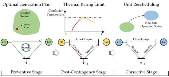
This paper proposes that the thermal inertia of transmission lines can be used to cope with post-contingency overflows in the conventional CSCOPF model. According to the system behavior, the post-contingency stage is divided into a response substage and a ramping substage in time sequence. In the previous substage, corrective measures have not been implemented while the power flow shows a step change. In the latter substage, the power flow variation is approximately described by a linear function with the adjustment of unit active power outputs. Based on the assumption of constant resistances and the linearization of the radiated heat loss function, analytical solutions about real-time temperatures in both substages are obtained from the HBE. An enhanced security-constrained OPF (ESCOPF) model is established on the basis of CSCOPF model where thermal rating constraints are integrated in the post-contingency stage. The objective of the established model is to minimize the generation cost. In order to effectively deal with this multi-stage optimization problem containing the quadratic objective function and nonlinear constraints, a solving strategy based on Benders decomposition is proposed. The original problem is decomposed into a master problem of the preventive control and two subproblems of the corrective feasibility check and the thermal rating check. Due to the independence between each contingency, the parallel algorithm can be implemented in solving those two subproblems. An equivalent time method is presented to build an explicit relationship between the highest conductor temperature and unit power outputs. In each iteration, corresponding Benders cuts are generated for infeasible contingencies and returned into the master problem. The final generation plan is obtained until those two checks are satisfied for all contingency scenarios. Numerical simulation results validate that the system security is markedly improved by considering the line thermal inertia in the post-contingency stage and the generation cost is just slightly higher than the result of CSCOPF model.
The main contributions of this paper are summarized as follows:
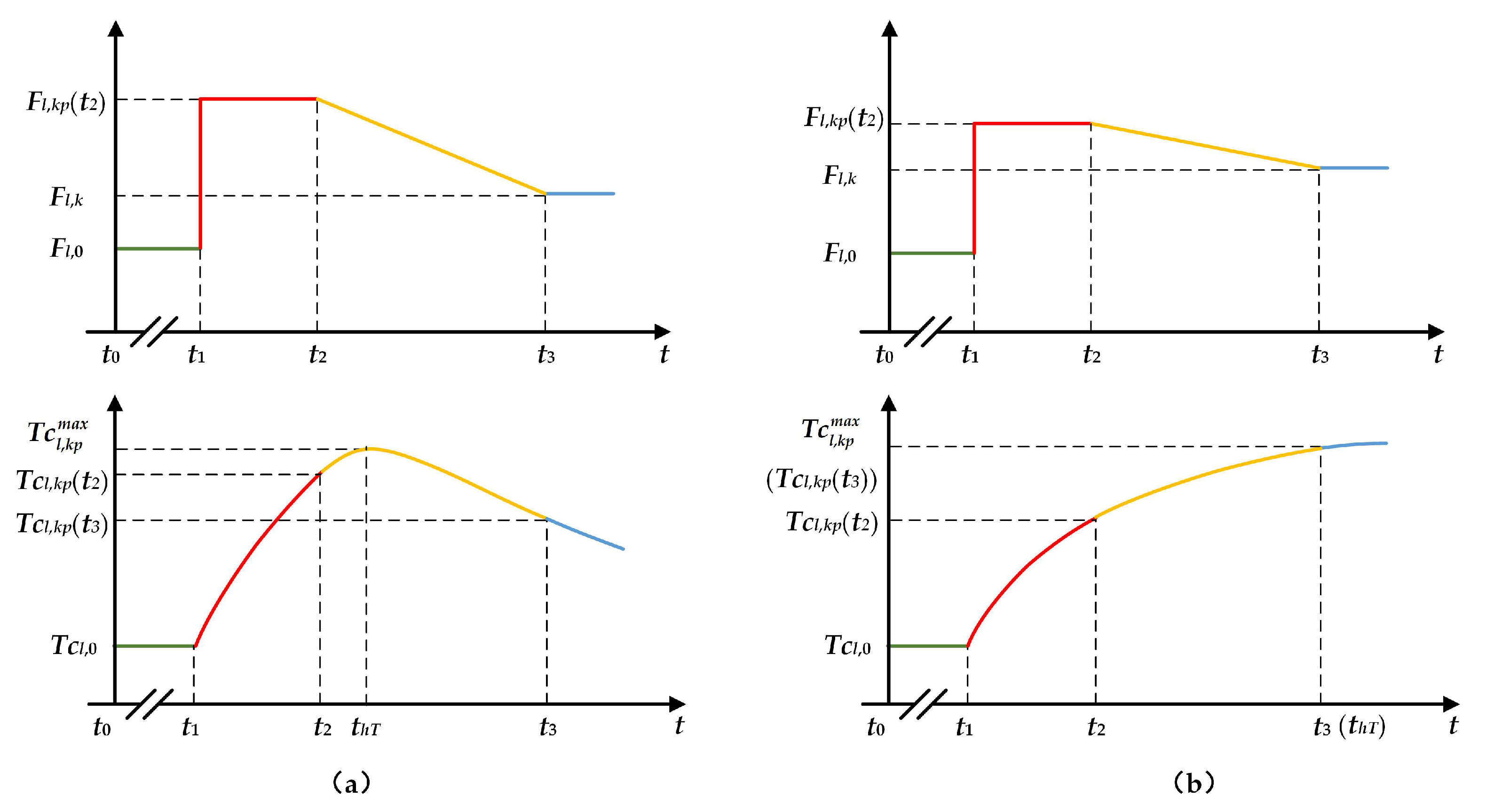
(a) Two typical temperature variations of post-contingency overload lines are analyzed and their analytical solutions are obtained. If the post-contingency power flow is significantly higher than the value in the corrective stage, the stationary point of the conductor temperature exists. Otherwise, its variation is monotonous.
(b) An ESCOPF model is established to minimize the system generation cost. Thermal rating constraints for line conductors are integrated in the post-contingency stage to avoid cascading failures. In addition, then, the unit rescheduling is implemented as the corrective measure to remove long-term overloads on transmission lines.
(c) A Benders decomposition based solving strategy is proposed to solve the ESCOPF model, which is divided into a master problem and two subproblems. In order to derive the partial derivative of the highest conductor temperature with respect to the unit active power output, an equivalent time method is presented.
The remainder of this paper is organized as follows.
Section 2 analyzes temperature variations of post-contingency overload lines and solutions of HBE in different stages are deduced. In
Section 3, the detailed formulation of ESCOPF model, which consists of the preventive stage, post-contingency stage and corrective stage, is presented. In
Section 4, a solving strategy based on Benders decomposition is proposed and the ESCOPF model is effectively solved by an iterative and parallel algorithm. Validities of the proposed model the solving strategy are verified on a 6-bus test system, a modified IEEE RTS-96 system, and a case 2383wp system in
Section 5. The main conclusions of this paper are drawn in
Section 6.
3. Enhanced Security-Constrained OPF
The enhanced security-constrained OPF model is established on the basis of the PSCOPF model. Thermal rating constraints are integrated in the post-contingency stage to improve the system security and the objective is to minimize the generation cost. Detailed formulations are presented as follows:
In the objective function (20), and denote the second order and the first order cost coefficients of unit i, respectively. indicates the fixed cost. is the active power output of the unit i determined by the preventive control. is the number of units. Because probabilities of contingencies are quite low and the rescheduling amount of power output is limited by unit ramping capacities, the cost of corrective control can be neglected.
Constraints (21)–(23) are utilized to guarantee the system operation security in the preventive stage. Equation (21) implies the active power balance where
is the load demand at the bus
j and
represents the number of load buses. Constraints (22) are power output limits where
and
denote the minimum and maximum power output of the unit
i, respectively. In power flow constraints (23),
and
are the preventive power output vector and the load demand vector, respectively.
and
indicate the rated power flow vector and the preventive power flow vector, respectively.
is the shift matrix in the base case without any failures. In the post-contingency stage, due to the change of grid topology caused by device outages, the power flow distribution is needed to be recalculated for each contingency. Constraint (24) indicates the power flow equation where
and
are post-contingency power flow vector and the shift matrix in the contingency
k, respectively. Conductor temperatures are limited by the constraint (25). According to the analysis of temperature variation in
Section 2, the highest temperature
in the post-contingency stage
k depends on
,
,
,
and
, and their functional relationships are determined by Equations (5)–(17).
Corrective control constraints consist of inequations (26)–(28). Constraints (26) and (27) indicate unit output limits in the corrective stage, where is the rescheduled power output of the unit i in the contingency k and is the adjustable power output determined by its reserve capacity. In the power flow constraint (28), denotes the corrective power flow vector and indicates the rescheduled power output vector in the contingency k. Line overloads must be completely eliminated by corrective measures and the power system enters a new safe operation status.
The established ESCOPF model is a multi-stage dispatch problem with the quadratic objective function (20) and nonlinear constraints (25). Due to the complex form of the temperature variation function in Equation (16), is presented as an implicit function about , , , and . This implies that conventional optimization methods could not be directly utilized to solve the established model, and some pretreatment measures need to be made. Moreover, different unit rescheduling plans are made for each contingency scenario. Therefore, the computational burden increases as the number of contingencies grows. It is necessary to control the solving time when applying the proposed model in large-scale power systems
4. Solving Strategy Based on Benders Decomposition
Benders decomposition is one of the commonly used decomposition techniques in power systems. J. F. Benders first introduced this decomposition algorithm for solving large-scale mixed-integer programming (MIP) problems [
37]. At present, it has been successfully applied to handle various optimization problems including the unit commitment [
38], economic dispatch [
39], and transmission planning [
40]. In applying Benders decomposition, the optimal solution may require iterations between the master problem and several subproblems. The lower bound and upper bound solution are provided by the master problem and feasible subproblems, respectively. If any of the subproblems is infeasible, a Benders cut will be introduced to the master problem. When the upper bound and the lower bound are sufficiently close, the iteration stops. In this section, a solving strategy based on Benders decomposition is presented to solve the established model with nonlinear thermal rating constraints.
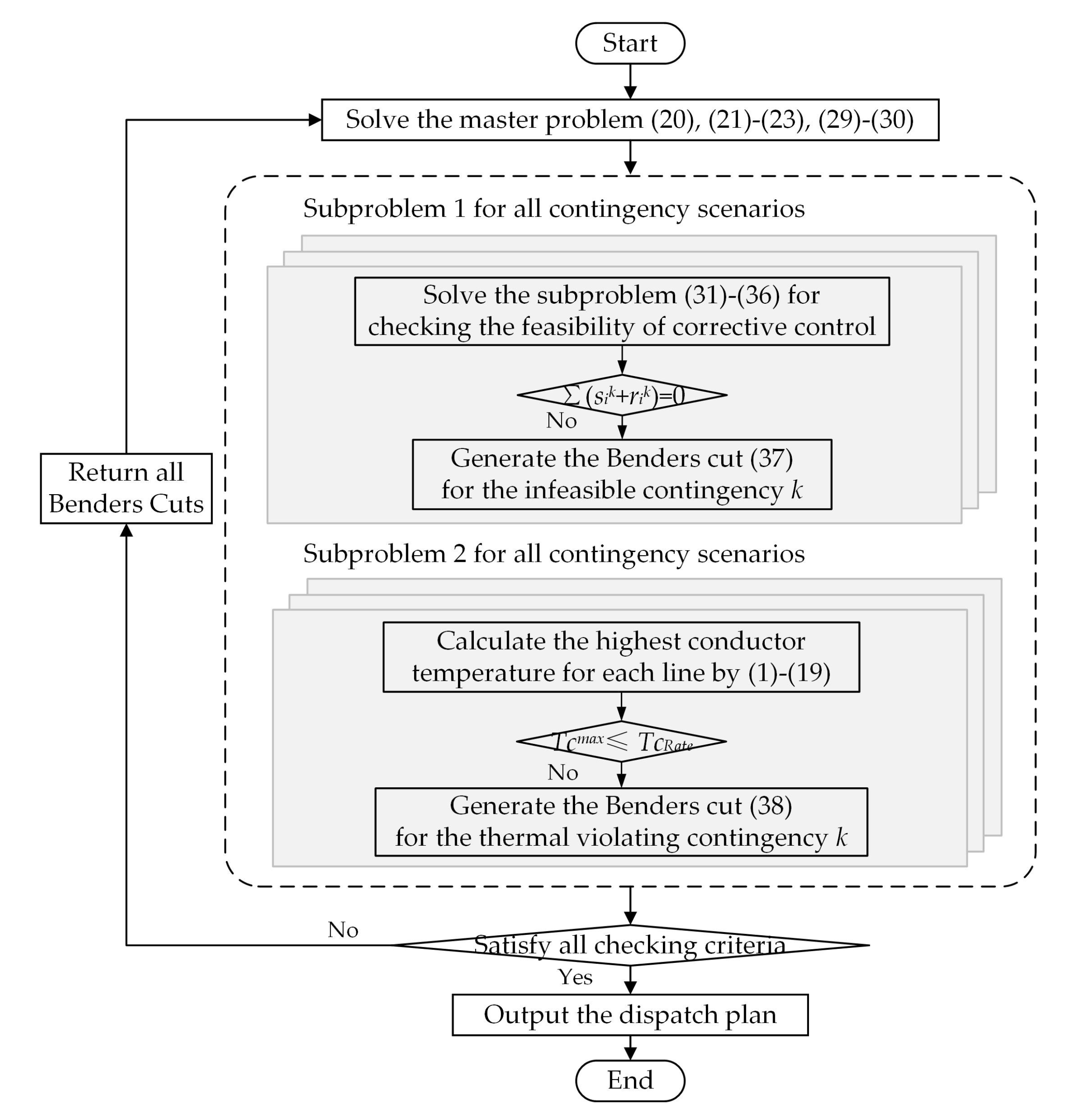
The ESCOPF model is first decomposed into a master problem optimizing the preventive control and two subproblems for the corrective control feasibility check and the line thermal rating check, respectively. In the second subproblem, conductor temperatures are calculated based on the determined power flow distribution in the preventive, post-contingency and corrective stage. Meanwhile, the independence between each contingency is taken into account and both subproblems can be processed in parallel. For those contingencies which cannot pass the corrective feasibility check or the line thermal rating check, corresponding Benders cuts are generated and returned into the master problem. The master problem and subproblems are sequentially solved until both checks are satisfied for all contingency scenarios. The specific solving flow is shown in
Figure 2 and detailed formulations for the master problem and two subproblems are presented as follows.
4.1. Master Problem (Preventive Control Optimization)
The preventive control problem is optimized separately in the master problem which consists of the objective function (20), constraints (21)–(23). The preventive power flow is obtained and the power flow redistribution in each contingency during the response stage can be calculated by Equation (24). Corresponding temperature variations from
to
are quantified by Equations (1) and (10). In each iteration, Benders cuts (29) and (30) are generated for those check violating contingencies and added into the master problem as constraints:
The feasible region of the master problem is continuously shrunk by returned Benders cuts and the most economical operating point is searched again in the new feasible region. According to following generating approaches for Benders cuts, above constraints (29) and (30) are linear. Therefore, the master problem in each iteration is a linearly constrained quadratic optimization problem which can be directly solved by current optimizers such as Cplex, Gurobi and so on.
4.2. Subproblem 1 (Corrective Control Feasibility Check)
Due to the existence of correlated constraints (27) between the preventive control and corrective control, the feasibility of corrective control needs to be checked for the operating point determined by the master problem in each iteration. In the credible contingency
k, slack variables
and
are introduced for power output rescheduling constraints. Detailed formulations of the corrective control feasibility check subproblem are presented as follows:
In the constraints (33) and (34), the determined preventive power output is a constant provided by results of the master problem in the current iteration. After solving the subproblems (31)–(36), the corrective power flow distribution is obtained and temperature variations after can be quantified by Equations (16) and (19).
Once the optimized result of the objective function (31) equals 0, overflows in the contingency
k can be eliminated by a feasible unit rescheduling. Otherwise, corresponding Benders cuts are needed to be generated and returned to the master problem. The Benders cut of the contingency
k which cannot be corrected is deduced as:
where
and
are the Lagrange multipliers of the constraint (33) and (34), respectively. The Benders cut (37) is a linear constraint about
where
,
,
,
and
are constants. Only if the optimized result of this subproblem equals 0 for all contingencies, the operating point set by the master problem can pass the feasibility check for the corrective control.
4.3. Subproblem 2 (Line Thermal Rating Check)
Temperature variations for four sequential stages are calculated based on the power flow variation determined by the master problem and the corrective control feasibility check subproblem. In each contingency, only if the highest temperature of each line conductor is below its rated value, the thermal rating check can be satisfied. Otherwise, the Benders cut is needed to be derived and added into the master problem:
where
denotes the set of transmission lines which violate thermal rating constraints. The key point of obtaining the thermal rating Benders cut is calculating the partial derivative of
with respect to
. In this paper, an equivalent time method is proposed to build an explicit relationship between the highest conductor temperature and the preventive power output.
The basic idea is using an extended response process to simulate the original two-stage process of the post-contingency temperature variation. The equivalent principle is that those two processes have the same highest temperature and the equivalent time
of the line
l in the contingency
k can be calculated from the following equation:
Due to the monotonous variation of the conductor temperature in the extended response process, the partial derivative of
with respect to
can be derived by the chain rule:
where
indicates the load current of the line
l at
in the contingency
k which can be obtained from results of the master problem. The partial derivative of
with respect to
can be calculated from the power flow Equation (24):
Similarly, based on the power flow equation in the preventive stage (23), the partial derivative of
with respect to
can be deduced as:
Using a quadratic function to fit the SHBE, the above partial derivation can be further derived as:
In Equation (44), denotes the determined preventive load current of the line l. It can be seen from the Equations (41)–(44) that the partial derivative of with respect to is a constant for the determined operating point and the unit rescheduling plan. This means the return Benders cut (38) is also a linear constraint.
The pseudocode of the solving strategy based on Benders decomposition is shown in Algorithm 1. It may help to reproduce and implement the approach proposed in this paper. The
and
indicate the number of contingenies which cannot pass the corrective control feasibility check and the line thermal rating check.
| Algorithm 1 The solving strategy based on Benders decomposition |
- Input:
Power system parameters and environment parameters. Durations of the response time and ramping time. The rated conductor temperature. The contingency set. - 1:
while and do - 2:
solve the master problem consisting of Equations (20), (21)–(23) and (29), (30); - 3:
obtain unit active output and power flow distribution ; - 4:
; - 5:
for each do - 6:
solve the subproblem 1 consisting of Equations (31)–(36); - 7:
if then - 8:
generate the Benders cut by Equation (37) and return it into th master problem; - 9:
obtain the power flow distribution ; ; - 10:
end if - 11:
end for - 12:
; - 13:
for each do - 14:
for each line l operating in the contingency k do - 15:
calculate the and by Equations (1)–(19) and (39), repsectively; - 16:
if then - 17:
add line l into the set - 18:
end if - 19:
end for - 20:
if then - 21:
; ; - 22:
for each do - 23:
; - 24:
end for - 25:
for each do - 26:
; - 27:
for each do - 28:
calculate the partial derivative by Equations (40)–(44); - 29:
; - 30:
end for - 31:
end for - 32:
return into the master problem; - 33:
end if - 34:
end for - 35:
end while - Output:
The active power output of each unit in the preventive stage and its adjusted amount in the corrective stage. The power flow distribution and variations of line conductors.
|
5. Case Studies
The model and solving strategy proposed in this paper are validated on a 6-bus test system, a modified IEEE RTS-96 system, and a case 2383wp test system. It assumed that all transmission lines in those three test systems use the 400 mm
Drake 26/7 ACSR conductor (Nexans S.A., Paris, France) whose parameters (resistance
R, diameter
D, heat capacity
and emissivity
) are given by Reference [
30] and shown in
Table 1.
Another assumption is that lines operate in the same environment condition, although it is difficult to be satisfied for large-scale power systems. The related environment parameters can be divided into two kinds. The air density
, dynamic viscosity
and the thermal conductivity of air
may not have obvious variations and could be regarded as constants. The other parameters including the ambient air temperature
, speed of air steam
, wind direction factor
and the power gain rate from the sun
can be provided by online micro-meteorology monitoring systems. With the development of smart grids, those systems have a wide range of applications [
41]. The more accurate measured parameters are obtained, the more effective control for the line thermal rating can be achieved. The data collected by distributed monitoring systems are transmitted through the high-speed optical networks or wireless networks like ZigBee, GPRS and 4G to energy management systems (EMS). Through data preprocessing, those data can be used to solve the electro-thermal coupling OPF model. Values of two kinds of parameters are presented in
Table 2.
In addition, for protection systems, the highest threshold value of line load current should be appropriately raised and the time-delay of triggering for overload lines needs to be increased. It will let protections not take action immediately and allow transmission lines to operate under the overload condition for a short period of time. In addition, then the ESCOPF model proposed in this paper can work in practical applications.
Under the condition of given parameters, the time constant of line thermal process is about 14 min which has been verified in Reference [
30]. Meanwhile, the rated load current of lines is set at 992 A while the corresponding steady-state temperature is 100.0
. The widely used “N−1” criterion is adopted for the former two test systems to filter line contingencies. This means, in each contingency, there is just a single transmission line outages. All simulations are performed on a personal computer with 4 Intel (R) Core (TM) i5-6200U CPU (2.3 GHz) (Lenovo, Beijing, China) and 8 GB memory. The programs are implemented using a Matlab (R2016a, The MathWorks, Natick, MA, USA) environment and underlying optimization problems are solved by Cplex.
5.1. 6-Bus Test System
The 6-bus test system consists of three units, three load bus, and 11 transmission lines. Its wiring diagram is presented in
Figure 3. Detailed parameters of units, load buses and lines are given by
Table A1,
Table A2 and
Table A3 (
Appendix A), respectively. There are 11 “N−1” contingencies where the line
k failures in the contingency
k. The response time and the ramping time of this system are 5 min and 7 min, respectively, and the rated conductor temperature is conservatively set at 100.00
. The mean program executing time of 10 tests with the consistent convergence solution is 10.07 s. Simulation results in each iteration are shown in
Table 3.
In the initial iteration, the preventive control is optimized separately with the lowest generation cost
$861.92. Four contingencies have post-contingency overflows which cannot be eliminated by the feasible corrective control. The thermal rating check is violated in three contingencies, and the highest temperature reaches 136.64
. Unit active power outputs are adjusted by returned Benders cuts as the iteration number grows. Combining with generation cost coefficients in
Table A1, it can be found that the output of the most expensive unit G2 increases, which results in the growth of
. It is worth noting that, after iteration 3,
increases from 0 to 1, while
decreases from 2 to 1. This implies that the corrective control feasibility check and the thermal rating check may be conflicting in some situations, and this conflict is solved by further shrinking the feasibility region of the operating point. After five iterations, both
and
drop to 0 and the highest conductor temperature is strictly controlled within the permissible scale 100.00
. This means that both short-term and long-term safe operation of this 6-bus system can be guaranteed. The final generation cost rises to
$917.51, which is 6.5% higher than its initial results.
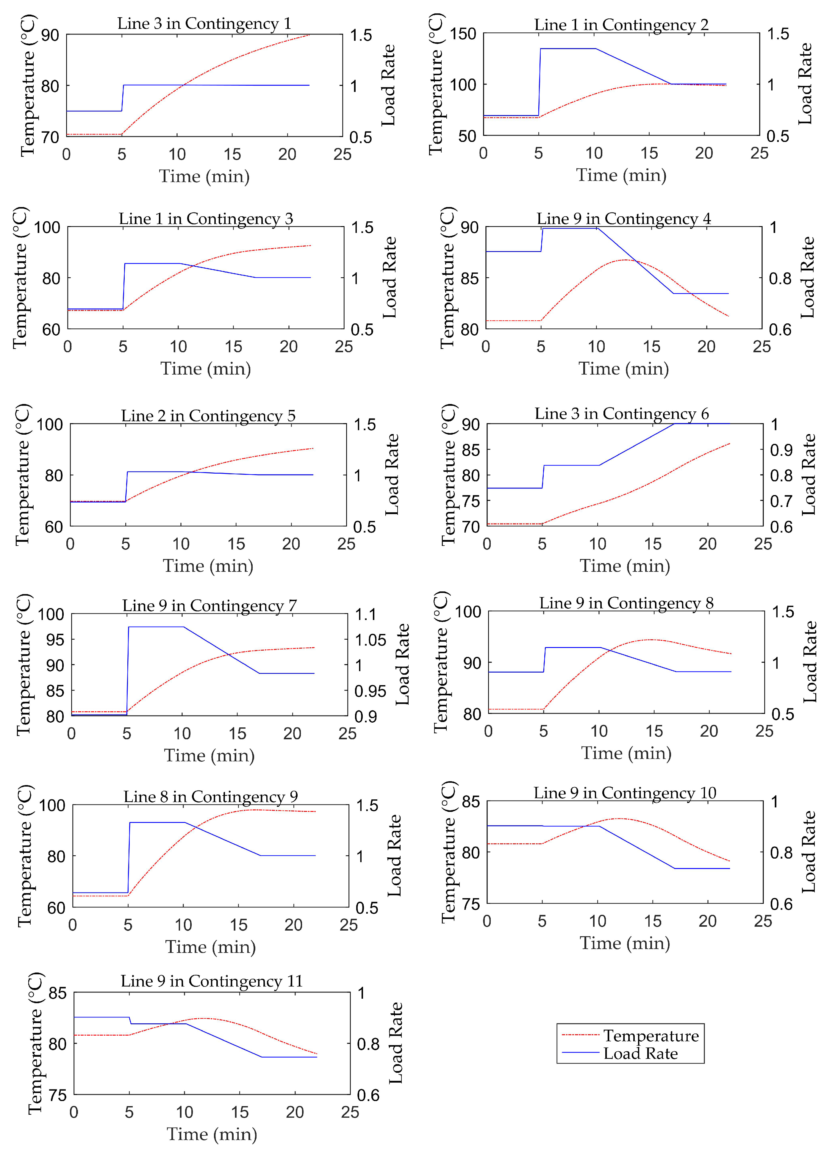
In addition, temperature variations of lines that have the highest conductor temperature in each contingency are shown in
Figure 4. Displayed durations of the preventive stage and the corrective stage are both 5 min. The post-contingency stage starts at the 5th min and ends at the 17th min. It is further confirmed that conductor temperatures in all contingencies are below the allowable value 100.00
. The highest temperature occurs on line 1, which connects two units G1 and G2 in the “N−1” contingency with the failure of line 2. The post-contingency load rate of line 1 reaches 1.35 at the 5th min and drops to 1.00 from the 10th min to the 17th min. The temperature rapidly rises to the peak 100.00
at around the 15th min and then slowly declines. This result verifies that the power flow constraint and the thermal rating constraint are not equivalent, and the former constraint is over conservative from the short-term perspective.
The conductor temperature varies monotonously under the condition that the corrective power flow is higher or slightly lower than it in the post-contingency stage. This corresponds to cases of the highest temperature line in the contingencies 1, 3, 5, 6, and 7. For those lines with highest temperature in the contingencies 2, 4, 8, 9, 10, and 11, the post-contingency power flow is significantly higher than the corrective value while concave temperature curves are presented. In those cases, the maximum absolute difference between load rates in the post-contingency and the corrective stage reaches 0.35, which is obviously higher than the value 0.14 in former cases. This result validates the analysis about two typical temperature variations in
Section 2.
It can be found from
Figure 4 that the highest temperature occurs five times on line 9 in 11 credible contingencies. Line 9 directly connects the unit G3 and the load bus L3 while the load rate in the preventive stage is 0.90. It is markedly higher than the second highest load rate 0.75 of line 3, which becomes the highest temperature line for the remaining two contingencies. From this perspective, line 9 can be regarded as the key transmission line in the 6-bus system while the security and economy of the system could be improved by appropriately raising its transmission capacity.
5.2. IEEE RTS-96 System
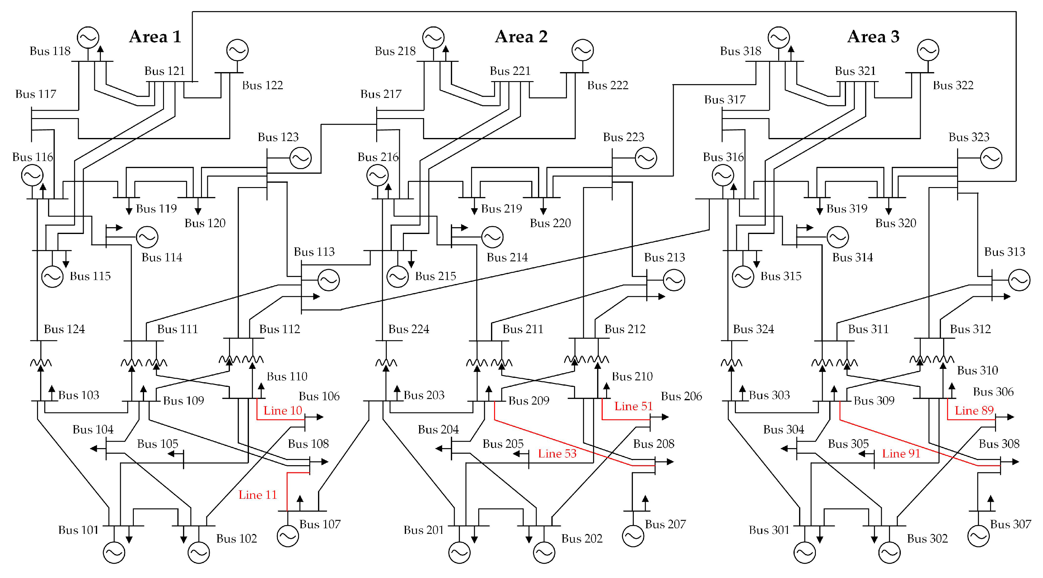
The modified RTS-96 system consists of three interconnected RTS-79 systems and has 96 units, 73 buses, and 120 branches in total. Its topology is presented in
Figure 5. The unit data and load data can be found in Reference [
42] while the modified line data are provided by Reference [
15]. Because line 52 in area 2 and line 90 in the area 3 are single-circuit lines connecting to the bus 207 and bus 307, respectively, their outages will cause a power imbalance in the post-contingency stage. Other measures such as more frequent inspections and maintenance could be used to improve their secure operations. Therefore, the final number of “N−1” line contingencies is 118.
In the base case, the response time and ramping time of this system are also set at 5 min and 7 min, respectively, while the rated conductor temperature is 100.00
. The mean value of the program executing time for 10 simulations with the same convergence solution equals 53.87 s and detailed simulation results in each iteration are shown in
Table 4.
There are 10 contingencies which cannot satisfy the corrective control feasibility check in the initial solution. Post-contingency overflows occur in all contingencies, and the highest load rate reaches 1.78. From the perspective of thermal rating, 19 contingencies are not secure. The highest temperature is 136.04
, and the lowest total generation cost is
$5058.8. After the first iteration,
,
, and
decrease significantly to 2, 53, and 8, respectively. In results after iteration 3,
approaches its final optimized value. This is because the same type of units have the same generation cost coefficients. Actually, the generation plan is still adjusted, which can be observed from variations of
,
,
, and
. After seven iterations, long-term overflows can be totally removed by the feasible corrective control while the highest temperature equals the rated value 100
, which confirm that the algorithm has converged. It is worth noting that there are still 51 contingencies having post-contingency overload lines. However, according to the analysis in
Section 2, those short-term power flow violations will not affect the operation security of transmission lines.
In order to further verify the effective control for conductor temperatures through the ESCOPF model, the highest conductor temperature of each transmission line in all credible contingencies is presented in
Figure 6.
It can be seen that most of temperatures are in the interval between 50 and 90 . The highest post-contingency temperature 100 occurs on line 10 and line 11, while temperatures of line 51, line 53, line 89, and line 91 are also very close to this limit. Based on the system diagram, it can be found that those lines are at similar topological locations in corresponding areas. For instance, line 10, line 51, and line 89 connect the bus 106 and bus 110, bus 206 and bus 210, bus 306 and bus 310, respectively. When focusing on the area 1, the 136 MW load demand is located at the bus 106. Once line 5 connecting bus 102 and bus 106 fails, 136 MW of power is needed to be transferred by line 10 alone. Meanwhile, the load rate of line 10 in the preventive stage 0.82 is relatively higher. The system operation security can be improved by controlling conductor temperatures of those key transmission lines in the post-contingency stage.
The performance of the proposed ESCOPF model is further compared with the conventional PSCOPF model and CSCOPF model from the perspective of security and economy, while detailed results are listed in
Table 5.
It can be seen that the PSCOPF is the most conservative model with the highest generation cost $5145.4. For the operating point obtained through this model, power flow constraints are satisfied for all contingencies. Since there is no post-contingency stage, the values of and do not exist. The CSCOPF model tries to eliminate overflows by the corrective control while effects of the time delay are ignored. Both power flow constraints and thermal rating constraints are violated in the post-contingency stage. The highest load rate and conductor temperature are 1.49 and 115.21 , respectively. Total generation cost $5063.6 is the lowest. In results of the proposed ESCOPF model, declines from 88 to 51 and is limited to 1.34. All credible contingencies can pass the thermal rating check. From the viewpoint of line dynamic thermal behavior, the ESCOPF model and the PSCOPF model have the equivalent security. However, the former total generation cost $5072.5 is just slightly higher than the result of CSCOPF model.
In addition, influences of the rated conductor temperature on the highest line load rate in all contingency scenarios and the total generation cost of the system are studied and results are shown in
Figure 7.
The highest load rate in the post-contingency stage increases while the total generation cost decreases as the rated conductor temperature grows. It can be observed that both rates of change decline. When the rated temperature is set at 88.53 , there is no contingency having overload lines, and the total generation cost equals the result of the PSCOPF model. Actually, the corrective control is no more needed while the ESCOPF model degenerates into a PSCOPF model. When the preset rated temperature is higher than 115.21 which is over the highest temperature occurring in results of the CSCOPF model, thermal rating constraints in the post-contingency stage become redundant. This means that the established ESCOPF model is converted into a CSCOPF model and their final optimized generation costs $5063.6 are consistent.
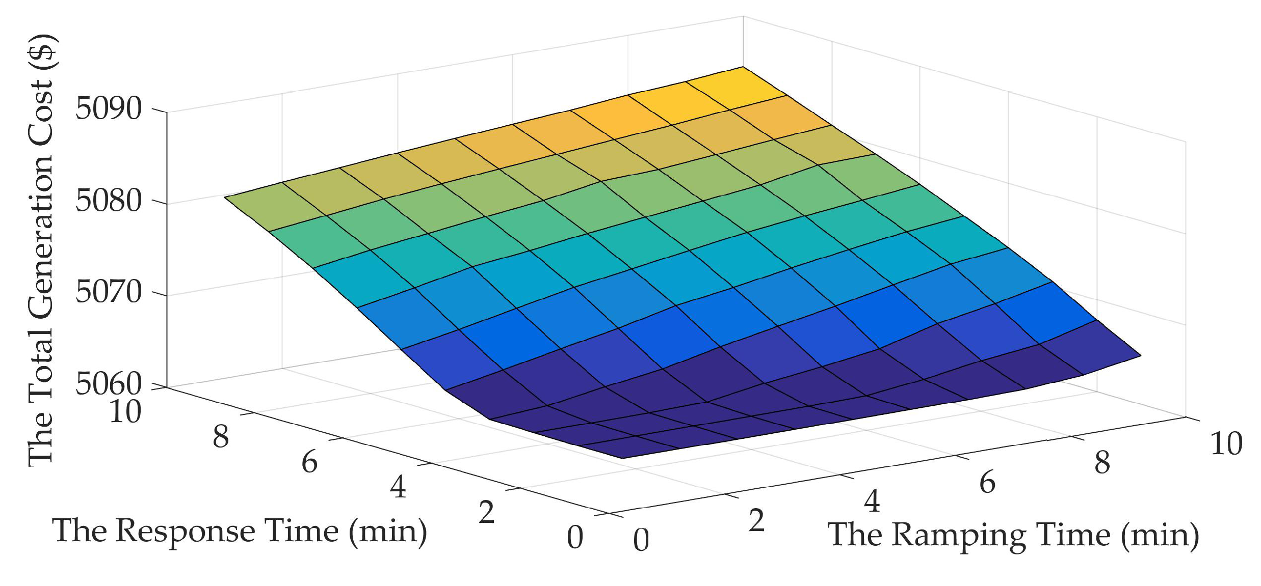
Moreover,
Figure 8 presents the surface of total generation costs under various combinations of the response time and the ramping time. The generation cost remains unchanged while the response time is below 3 min and the ramping time is within 5 min. Due to the thermal inertia, lines can operate under extremely high load rates and do not violate thermal rating limits for a short duration. The operating point of the system is not affected by post-contingency thermal rating constraints. As both growths of the response time and the ramping time, the generation cost continues increasing. It can be observed that the variation of the response time has a greater influence. This is because the post-contingency power flow keeps up a high level in this duration. While the response time is in the interval of 5–8 min and the ramping time is within the interval of 6–9 min, the increase of the total generation cost is the most significant. Beyond this time interval, the growth becomes slow. The above analysis implies that shortening the system response time and implementing units with the quick ramping capacities can improve the security of power systems and decline its operating cost.
5.3. Case 2383wp Test System
In order to verify the validities of the proposed ESCOPF model and solving strategy on large-scale power systems, the case 2383wp test system that consists of 2383 buses, 2896 branches, and 327 units is adopted. Its detailed system parameters can be found in the file provided by Matpower (6.0, Cornell University, Ithaca, NY, USA). In addition, the ”N−5” contingencies are randomly generated for simulations. It means that there are five failure transmission lines in each contingency. The rated conductor temperature is set at 100.00
for all lines. Simulations are conducted for 10, 20, 50 and 100 “N−5” contingencies and the executing time is 367.83 s, 547.76 s, 1817.73 s, and 4540.95 s, respectively. The detailed results are shown in
Table 6,
Table 7,
Table 8 and
Table 9.
It can be found that the algorithm can converge quickly and steadily for the four simulations above within 8 iterations. The executing time increases with the growth of the number of contingencies. Those results are obtained on a person computer with series computation. According to the analysis in
Section 4, both subproblems can be processed in parallel due to the independence between each contingency. Therefore, when the model and algorithm are applied on more large-scale contingency sets, the parallel computing architecture can be used to effectively decline the executing time.
In initial solutions, maximum load rates reach around 8.00 and corresponding highest conductor temperatures are over 1200 . Both indicators are gradually controlled and decrease significantly as the iterations progress. In final convergence solutions, maximum load rates decline to around 1.6 while the highest temperatures are below the rated value 100.0 . For optimized operating points, all contingencies can pass the corrective control feasibility check and line thermal rating check. It also needs to be noted that the total generation cost increases from $27,027 to $33,593 with the growth of the number of “N−5” contingencies. This is because the feasible region of the power system is shrunk by adding more credible contingencies.
6. Conclusions
In this paper, an ESCOPF model where thermal rating constraints are integrated to limit post-contingency conductor temperatures is established. After the contingency occurrence, the system first experiences a response stage and a ramping stage in time sequence. Due to the thermal inertia, lines can transfer the power flow that is much higher than the rated value while conductor temperatures are still within the safe scale. The corrective control is implemented with a time delay and long-term overflows are eliminated.
A solving strategy based on Benders decomposition is proposed to deal with the ESCOPF model. The original dispatch problem is divided into a master problem and two subproblems. The system operating point is determined in the master problem while the corrective control feasibility check and the line thermal rating check are separately conducted in two subproblems. The partial derivative of the highest temperature with respect to unit power output in the thermal rating Benders cut is calculated by a presented equivalent time method.
Simulation results on a 6-bus test system, a modified IEEE RTS-96 system, and a case 2383wp test system demonstrate that proposed approaches can offer the following advantages:
(a) The solving strategy based on Benders decomposition steadily converges within eight iterations for three test systems. The finally obtained operating point can pass the feasibility check and thermal rating check and has the lowest generation cost.
(b) The explicit relationship between the highest temperature and unit power output can be built by the proposed equivalent time method. Post-contingency temperatures of line conductors are strictly controlled below the prescribed limit.
(c) The proposed ESCOPF model can find a better balance between the security and economy compared with the conventional SCOPF model. As rated temperatures decline, the model gradually degenerates into the PSCOPF model. Conversely, the obtained operating point approaches the result of the CSCOPF model.
(d) The generation cost increases rapidly as the duration of the response stage rises. Shortening the system duration in the response stage can significantly extend the safe operation region of systems and decrease the total generation cost.
The proposed ESCOPF model is based on the DC power flow which will cause the underestimation of actual conductor temperatures of transmission lines and a more accurate model is needed to be established. In addition, just like the conventional PSCOPF model and CSCOPF model, the ESCOPF model proposed in this paper is a tool that can be used to make the day-ahead, real-time generation plan, and so on. Therefore, a lot of work such as applying this model into the electricity market operation and power systems with the larger-scale renewable energy integration need to be done in future research.


