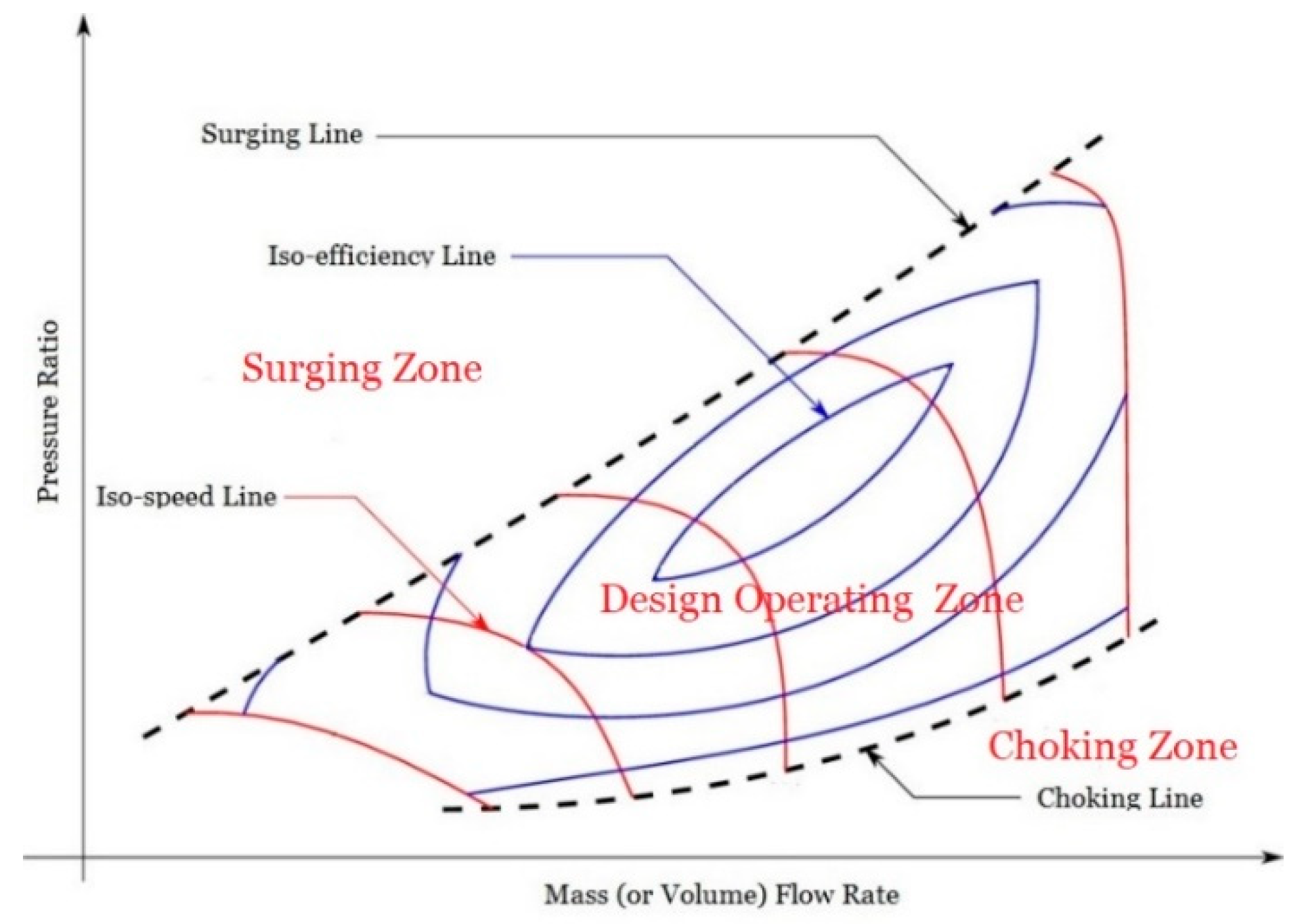
Figure 1.
Compressor performance map.
Figure 1.
Compressor performance map.
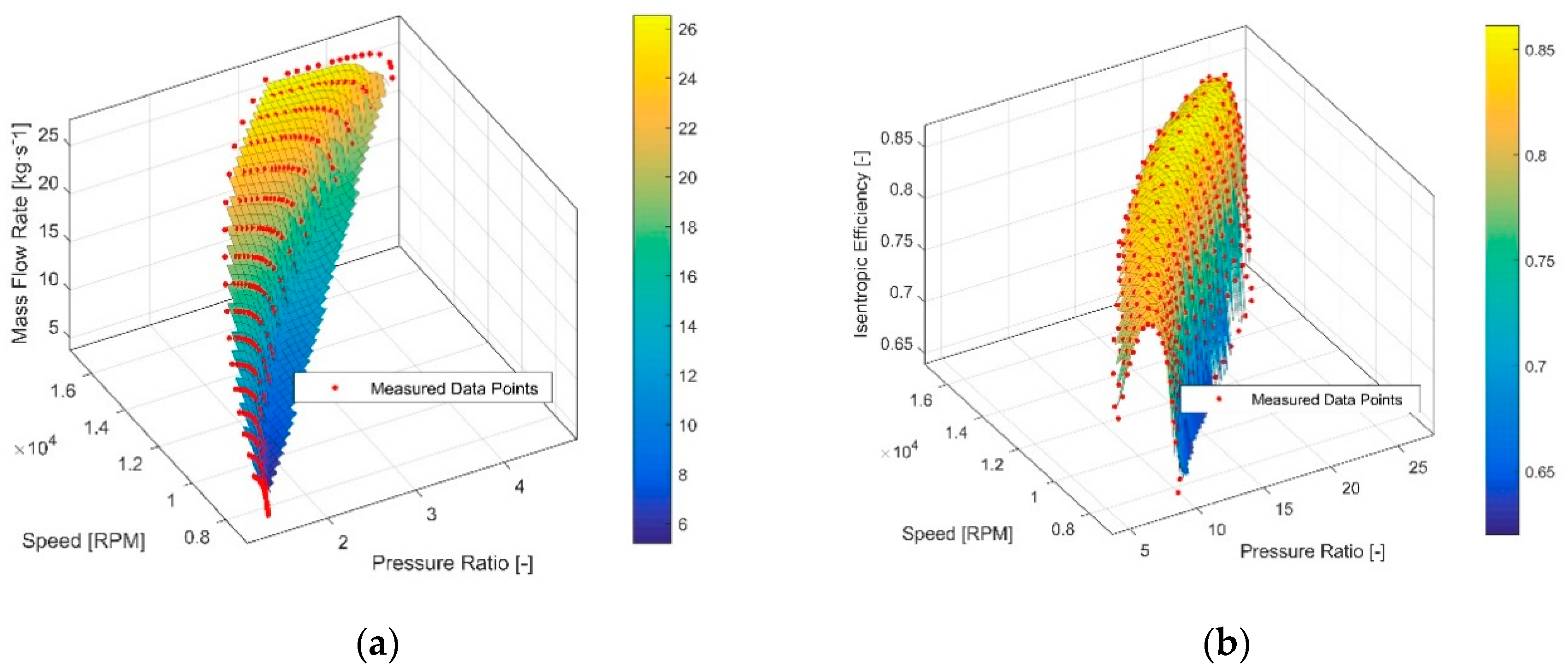
Figure 2.
Two-dimensional interpolation meshes constructed by look-up table method: (a) mass flow rate model; (b) isentropic efficiency model.
Figure 2.
Two-dimensional interpolation meshes constructed by look-up table method: (a) mass flow rate model; (b) isentropic efficiency model.
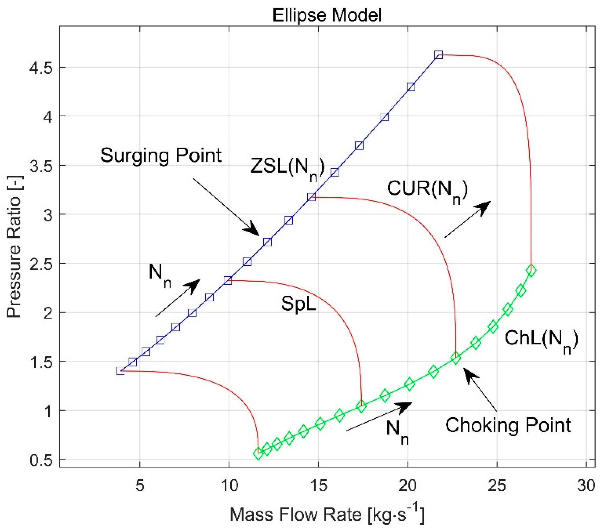
Figure 3.
Sketch of the main characteristics of the Leufvén and Llamas ellipse model.
Figure 3.
Sketch of the main characteristics of the Leufvén and Llamas ellipse model.
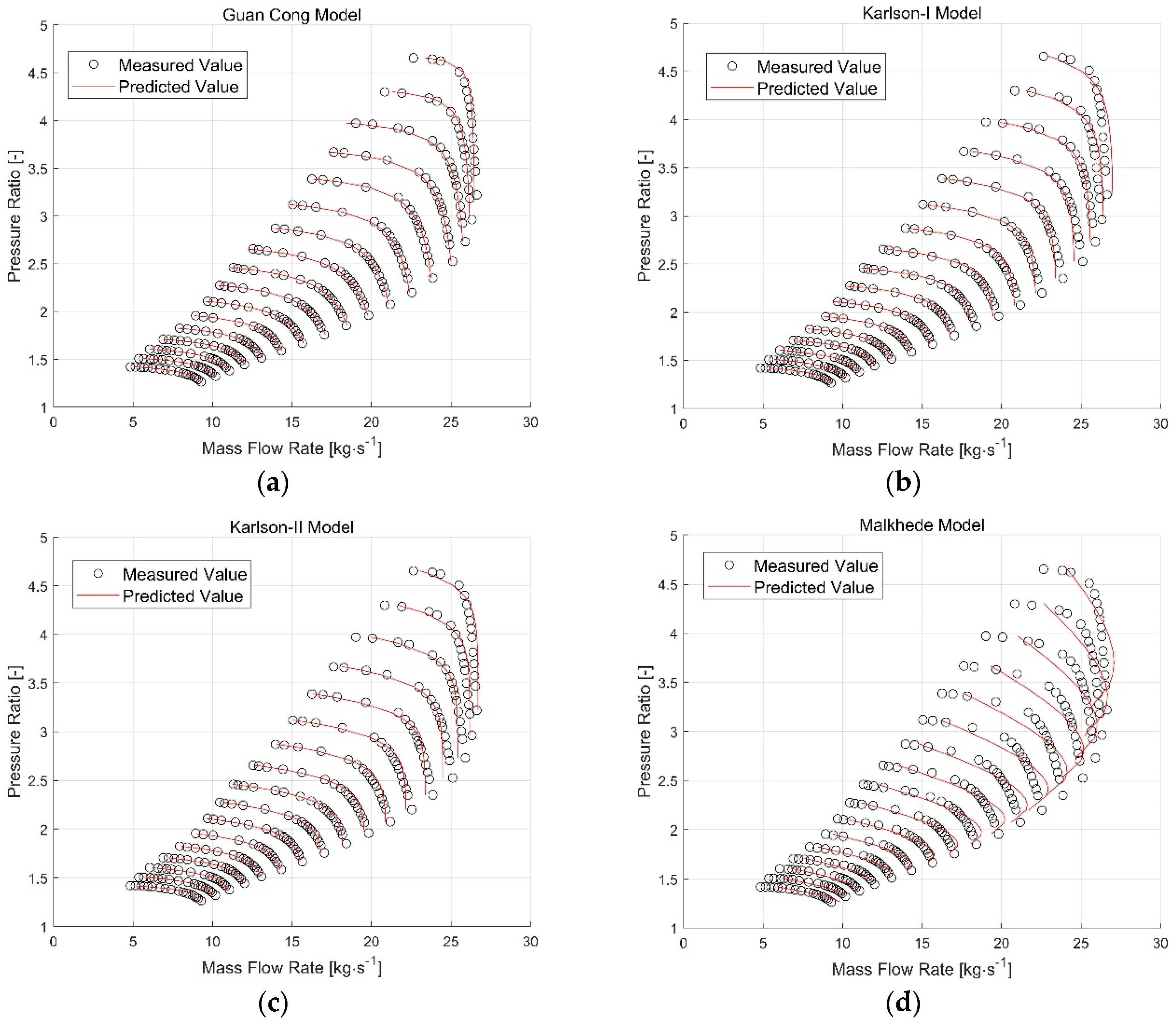
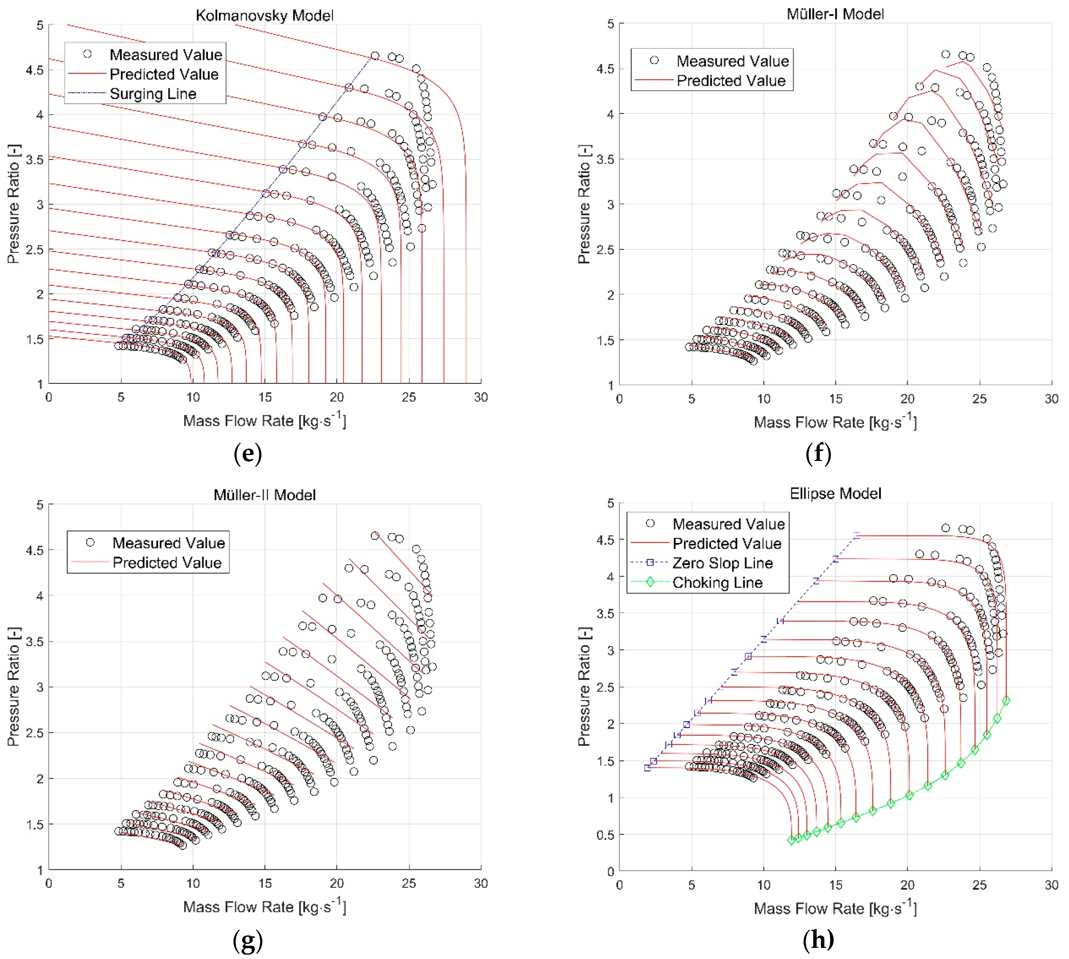
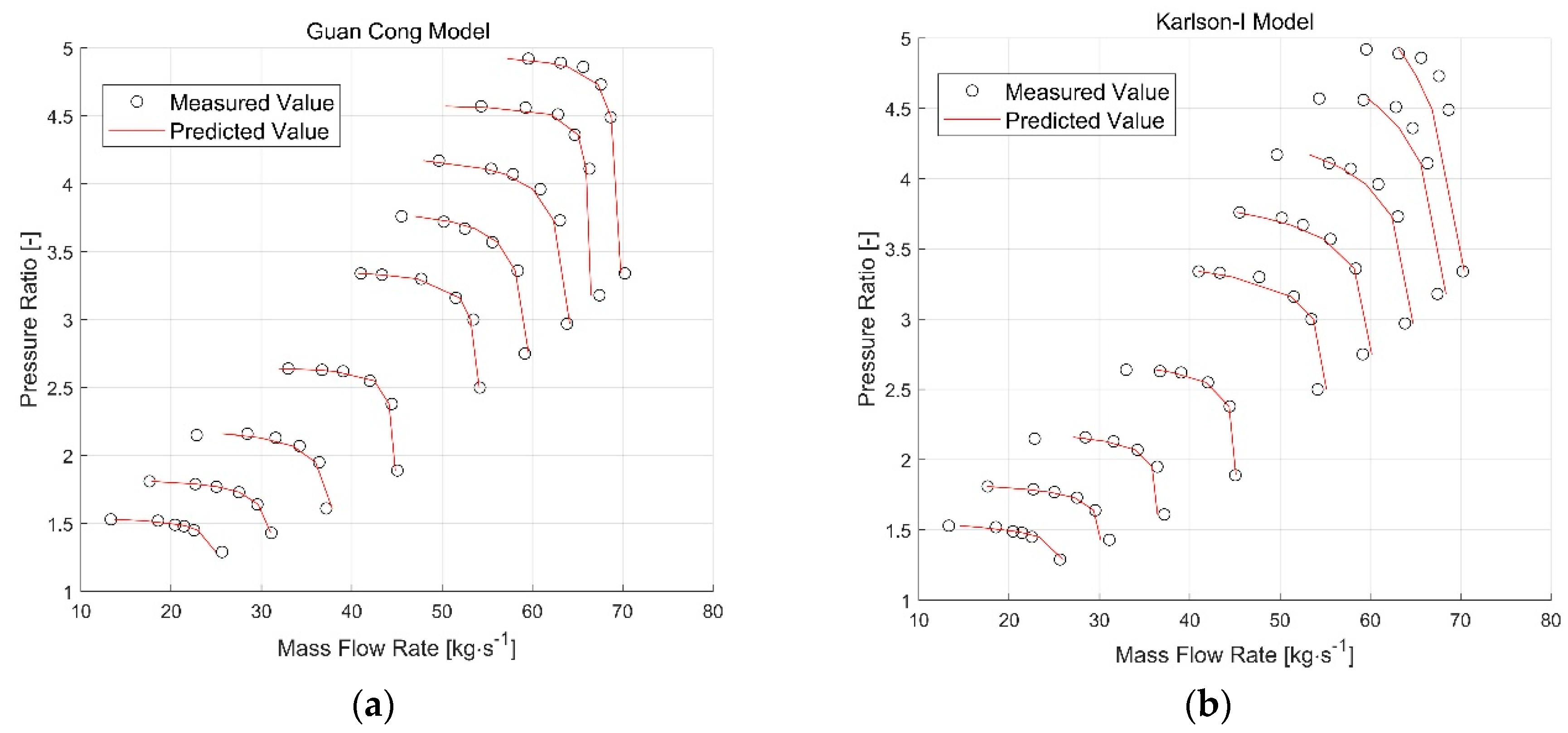
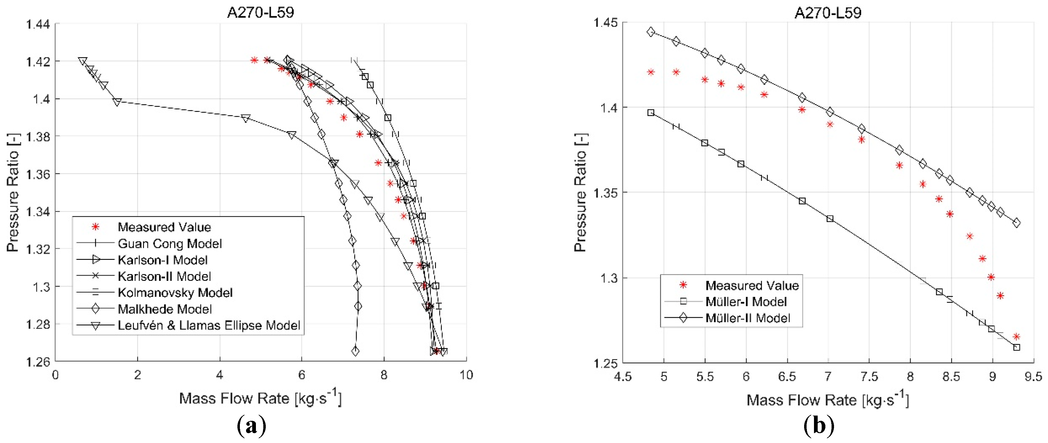
Figure 4.
Prediction results of each compressor mass flow rate model in design operating area for the A270-L59 compressor: (a) the Guan Cong model; (b) the Karlson-I model; (c) the Karlson-II model; (d) the Malkhede model; (e) the Kolmanovsky model; (f) the Müller-I model; (g) the Müller-II model; and (h) the Leufvén and Llamas ellipse model.
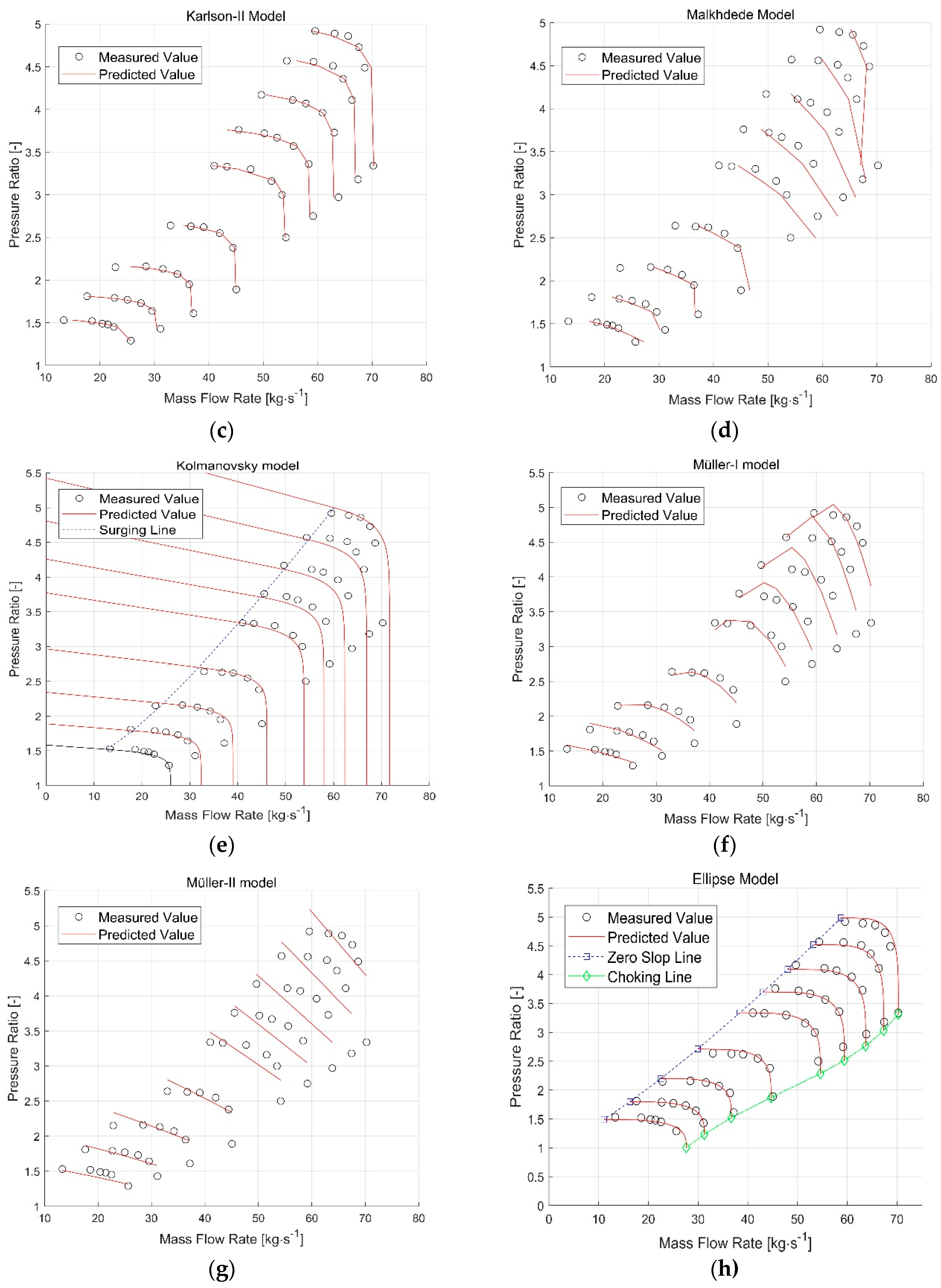
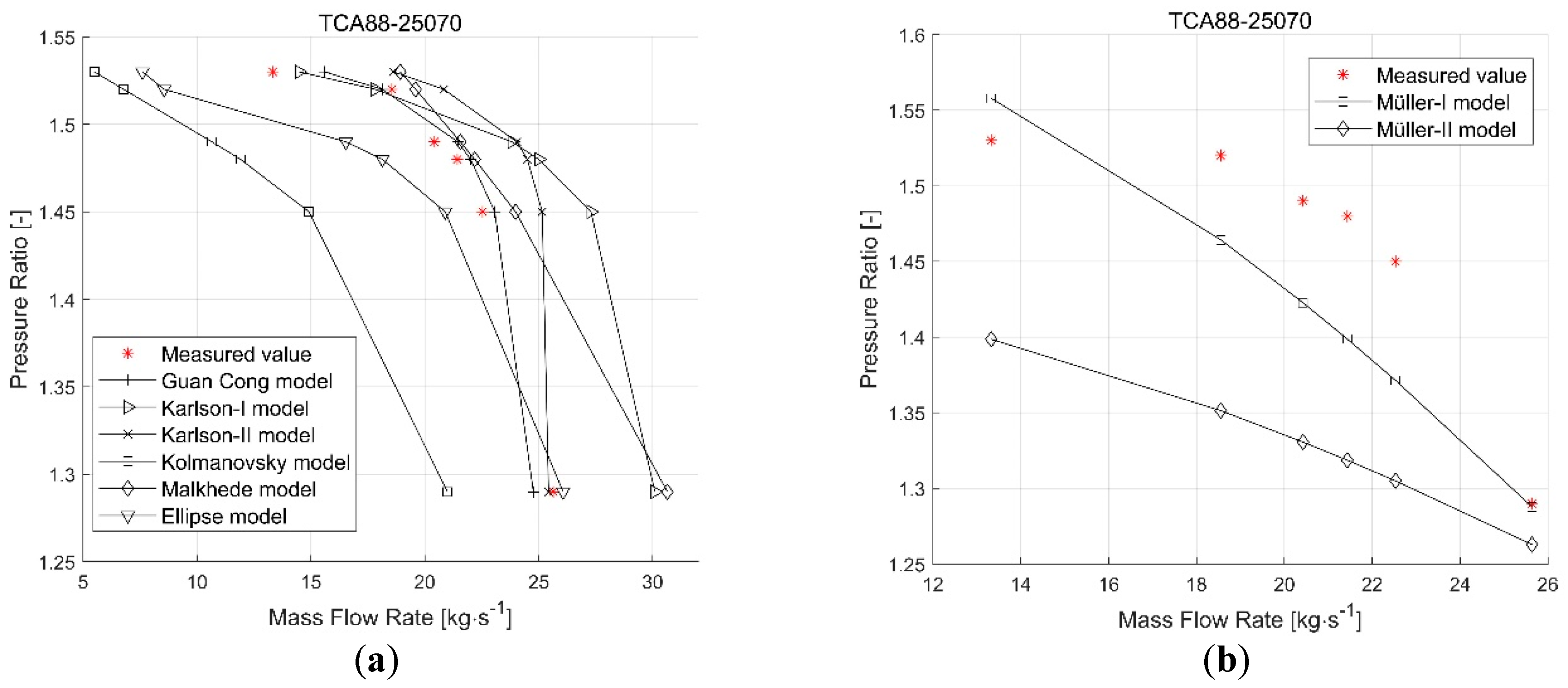
Figure 5.
Prediction results of each compressor mass flow rate model in design operating area for the TCA88-25070 compressor: (a) the Guan Cong model; (b) the Karlson-I model; (c) the Karlson-II model; (d) the Malkhede model; (e) the Kolmanovsky model; (f) the Müller-I model; (g) the Müller-II model; and (h) the Leufvén and Llamas ellipse model.
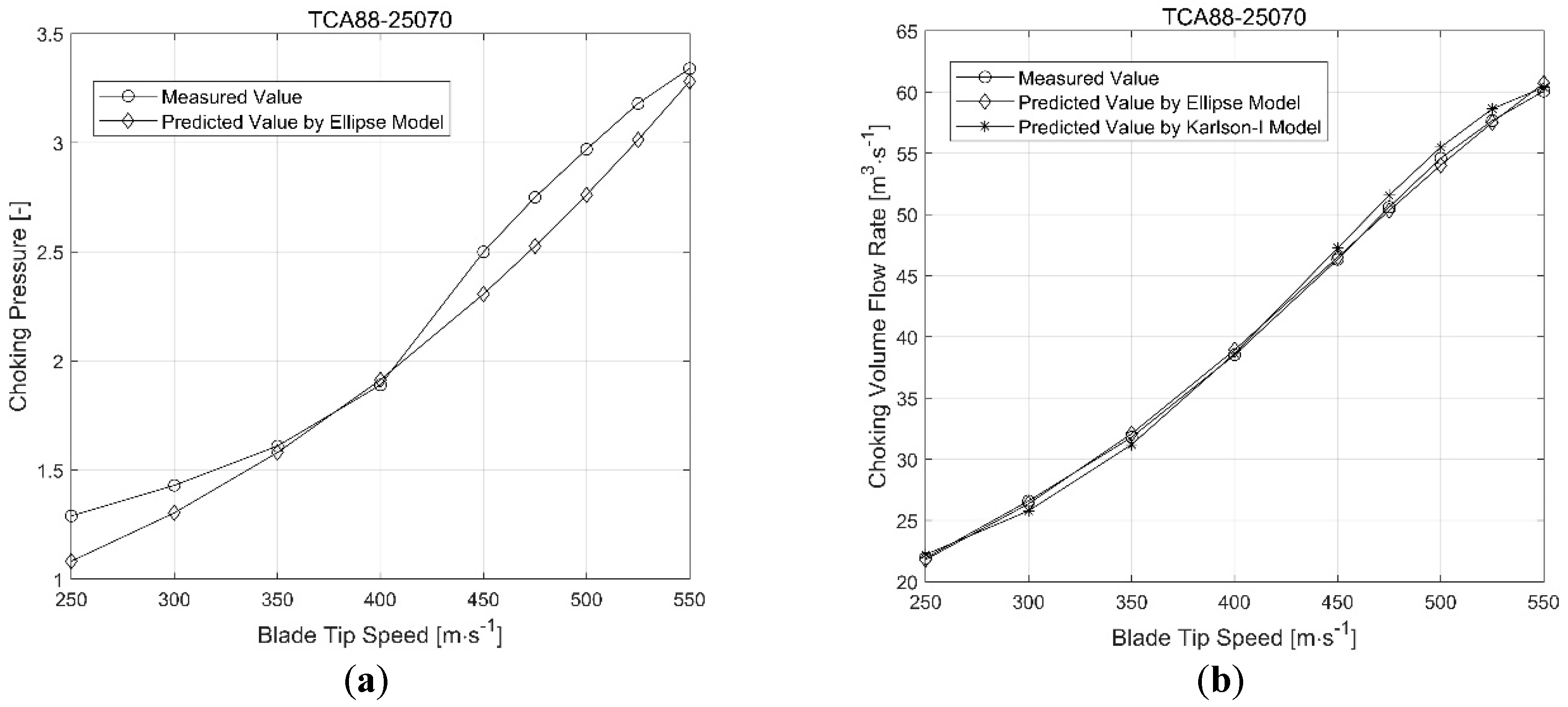
Figure 6.
Measured and predicted choking pressure and volume flow rate: (a) choking pressure; (b) choking volume flow rate.
Figure 6.
Measured and predicted choking pressure and volume flow rate: (a) choking pressure; (b) choking volume flow rate.
Figure 7.
LS area extrapolation results for each compressor mass flow rate model for the A270-L59 compressor: (a) model structure of ; (b) model structure of .
Figure 7.
LS area extrapolation results for each compressor mass flow rate model for the A270-L59 compressor: (a) model structure of ; (b) model structure of .
Figure 8.
LS area extrapolation results for each compressor mass flow rate model for the TCA88-25070 compressor: (a) model structure of ; (b) model structure of .
Figure 8.
LS area extrapolation results for each compressor mass flow rate model for the TCA88-25070 compressor: (a) model structure of ; (b) model structure of .
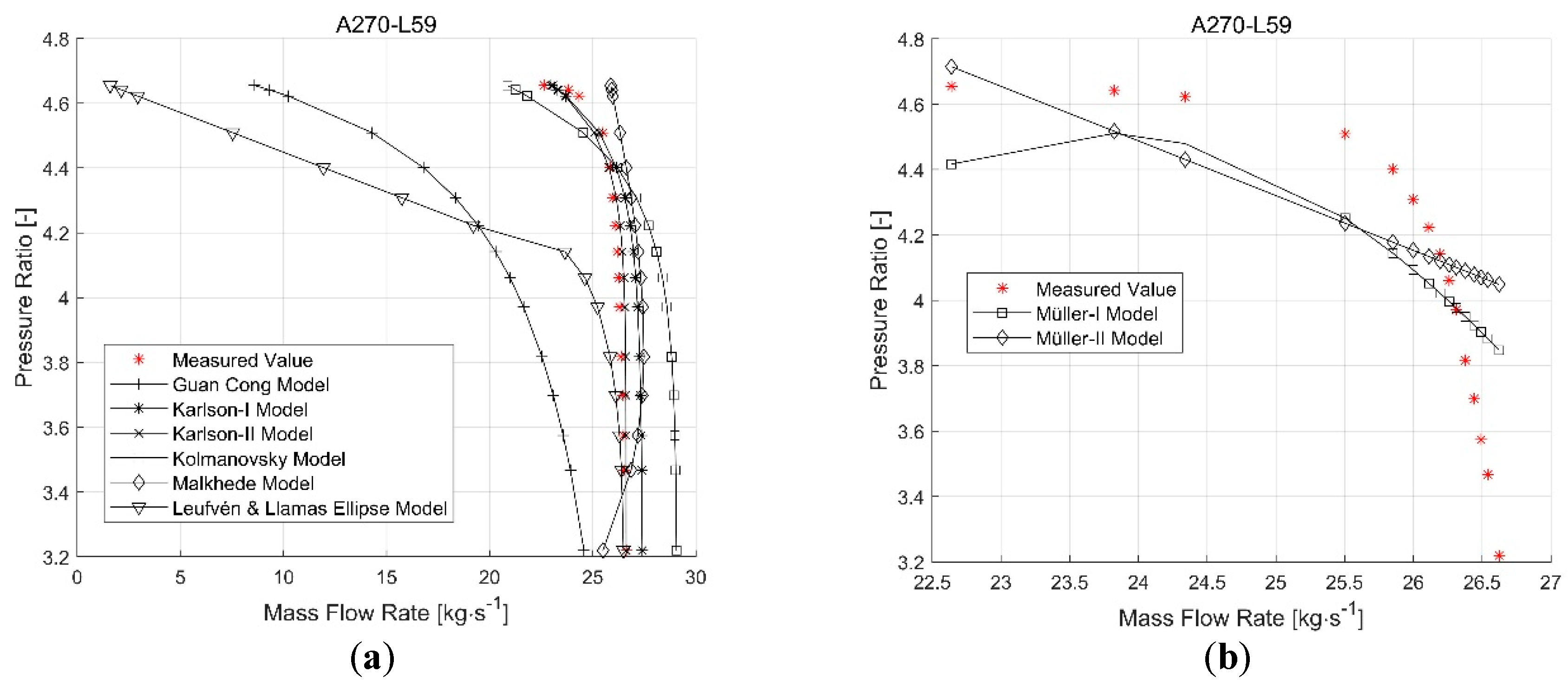
Figure 9.
HS extrapolation results for each compressor mass flow rate model for the A270-L59 compressor: (a) model structure of ; (b) model structure of .
Figure 9.
HS extrapolation results for each compressor mass flow rate model for the A270-L59 compressor: (a) model structure of ; (b) model structure of .
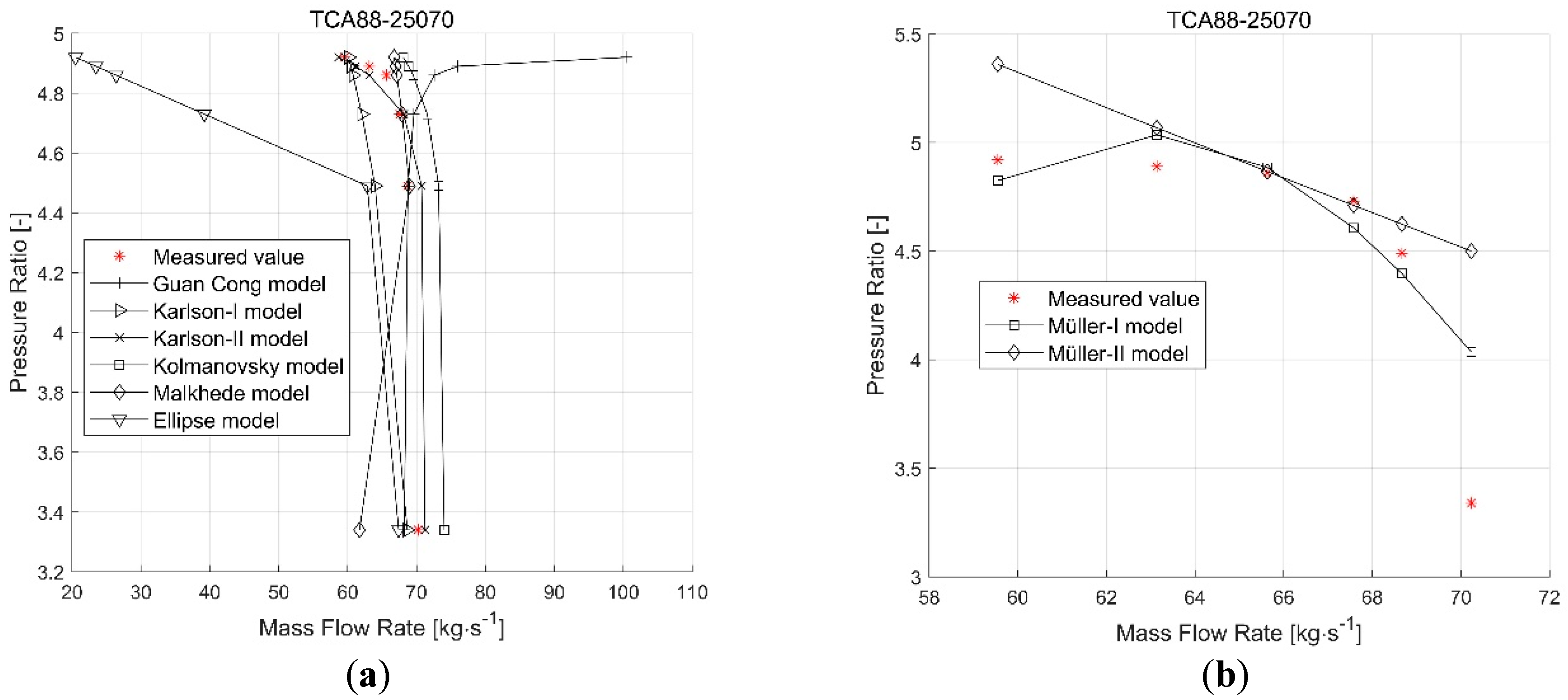
Figure 10.
HS area extrapolation results for each compressor mass flow rate model for TCA88-25070 compressor: (a) model structure of ; (b) model structure of .
Figure 10.
HS area extrapolation results for each compressor mass flow rate model for TCA88-25070 compressor: (a) model structure of ; (b) model structure of .
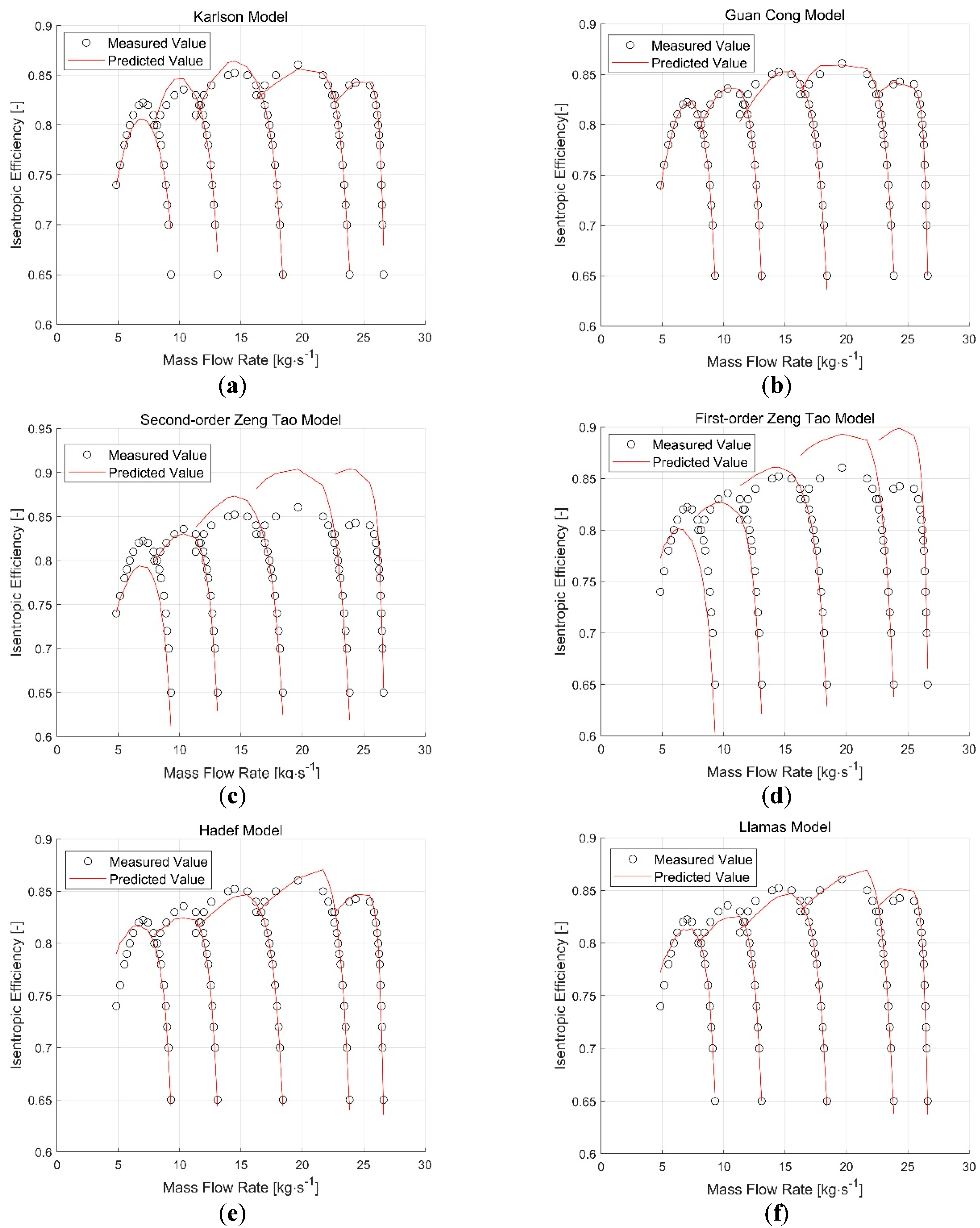
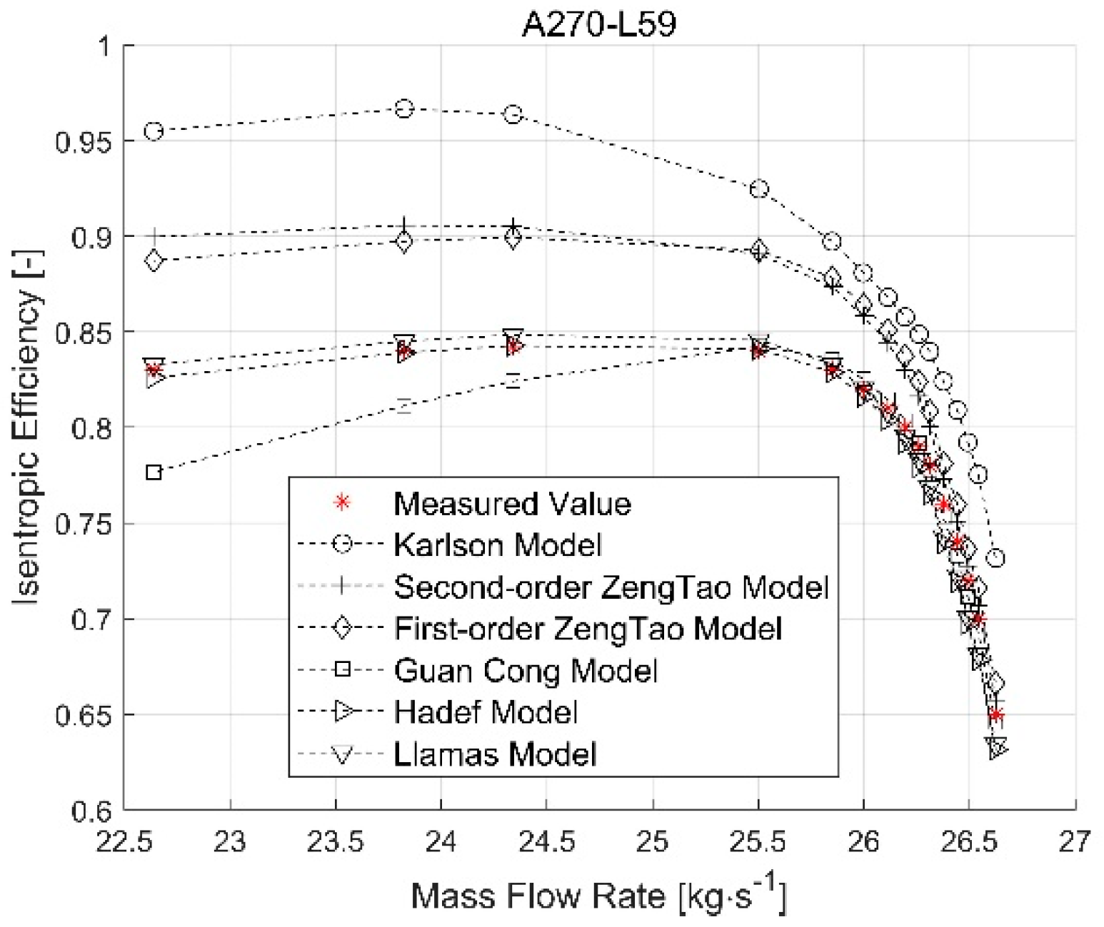
Figure 11.
Prediction results of each compressor isentropic efficiency model in design operating area for the A270-L59 compressor: (a) the Karlson model; (b) the Guan Cong model; (c) the Second-order Zeng Tao model; (d) the First-order Zeng Tao model; (e) the Hadef model; (f) and the Llamas model.
Figure 11.
Prediction results of each compressor isentropic efficiency model in design operating area for the A270-L59 compressor: (a) the Karlson model; (b) the Guan Cong model; (c) the Second-order Zeng Tao model; (d) the First-order Zeng Tao model; (e) the Hadef model; (f) and the Llamas model.
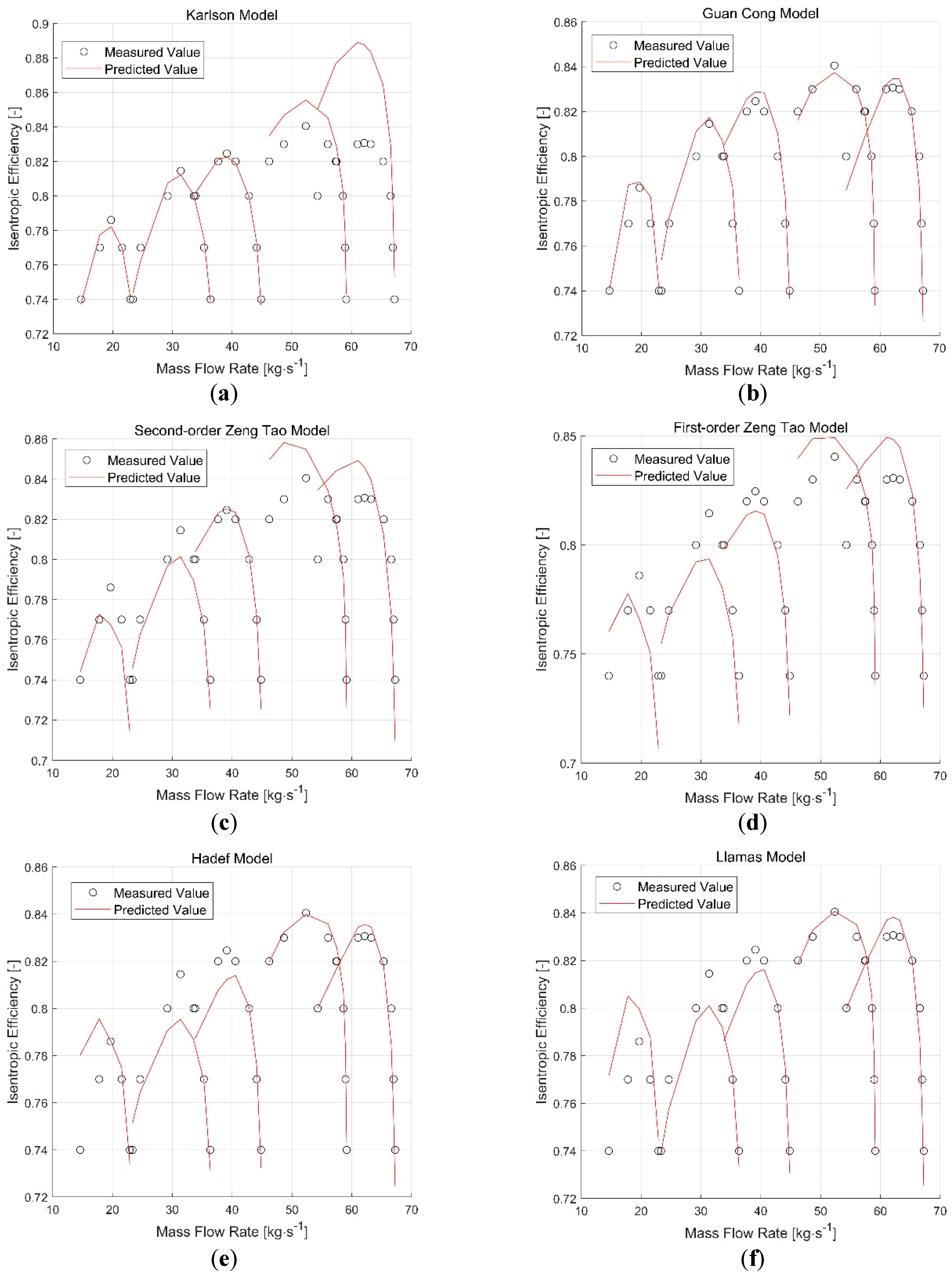
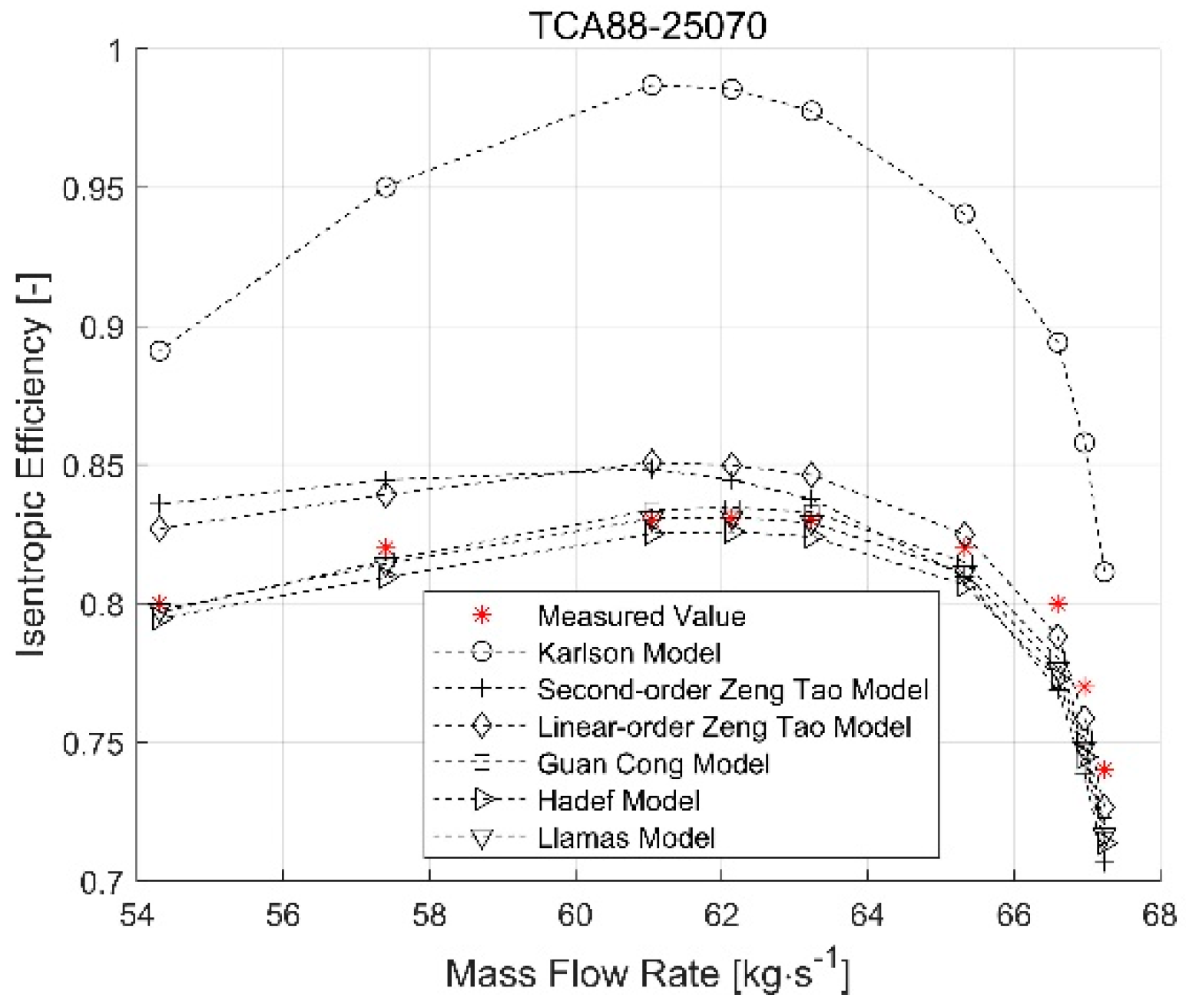
Figure 12.
Prediction results of each compressor isentropic efficiency model in the design operating area for the TCA88-25070 compressor: (a) the Karlson model; (b) the Guan Cong model; (c) the Second-order Zeng Tao model; (d) the First-order Zeng Tao model; (e) the Hadef model; (f) and the Llamas model.
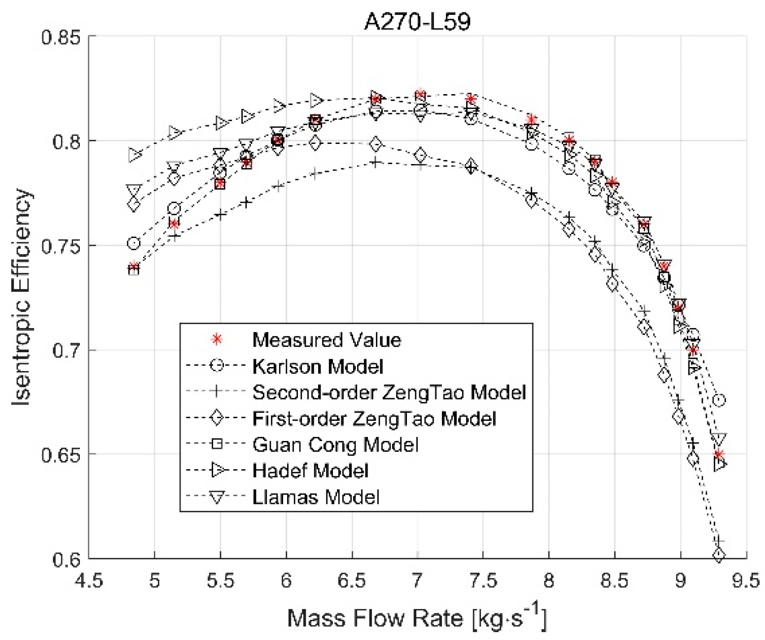
Figure 13.
LS area extrapolation results for each compressor isentropic efficiency model for the A270-L59 marine compressor.
Figure 13.
LS area extrapolation results for each compressor isentropic efficiency model for the A270-L59 marine compressor.
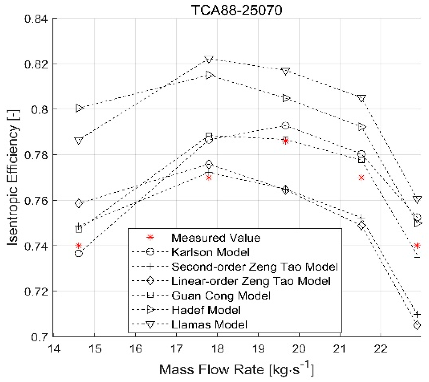
Figure 14.
LS area extrapolation results for each compressor isentropic efficiency model for the TCA88-25070 marine compressor.
Figure 14.
LS area extrapolation results for each compressor isentropic efficiency model for the TCA88-25070 marine compressor.
Figure 15.
HS area extrapolation results for each compressor isentropic efficiency model for the A270-L59 marine compressor.
Figure 15.
HS area extrapolation results for each compressor isentropic efficiency model for the A270-L59 marine compressor.
Figure 16.
HS area extrapolation results for each compressor isentropic efficiency model for the TCA88-25070 marine compressor.
Figure 16.
HS area extrapolation results for each compressor isentropic efficiency model for the TCA88-25070 marine compressor.
Table 1.
Main technical parameters of the A270-L59 and the TCA88-25070 marine compressors.
Table 1.
Main technical parameters of the A270-L59 and the TCA88-25070 marine compressors.
| Type | A270-L59 | TCA88-25070 |
|---|
| Impeller Diameter (m) | 0.59 | 0.893 |
| Maximum Flow in the Map (m3/s) | 23 | 60 |
| Maximum Speed in the Map (RPM) | 16,800 | 11,763 |
Table 2.
Error evaluation results of each compressor mass flow rate model in the design operating area for the A270-L59 compressor.
Table 2.
Error evaluation results of each compressor mass flow rate model in the design operating area for the A270-L59 compressor.
| Mathematical Model | (-) | MAPE (%) | (%) | (%) |
|---|
| Guan Cong model | 0.9996 | 0.5565 | 100 | 100 |
| Karlson-I model | 0.9989 | 1.0055 | 98.9619 | 99.6540 |
| Karlson-II model | 0.9989 | 0.9106 | 99.3080 | 100 |
| Malkhede model | 0.9905 | 3.2034 | 82.0069 | 97.9239 |
| Kolmanovsky model | 0.9890 | 3.3850 | 82.0069 | 92.7336 |
| Müller-I model | 0.9864 | 2.1315 | 89.2734 | 98.9619 |
| Müller-II model | 0.9714 | 3.5198 | 77.5087 | 95.8478 |
| Ellipse model | 0.9133 | 6.8087 | 77.8547 | 84.7751 |
Table 3.
Error evaluation results of each compressor mass flow rate model in the design operating area for the TCA88-25070 compressor.
Table 3.
Error evaluation results of each compressor mass flow rate model in the design operating area for the TCA88-25070 compressor.
| Mathematical Model | (-) | MAPE (%) | (%) | (%) |
|---|
| Guan Cong model | 0.9926 | 2.2779 | 88.8889 | 98.1481 |
| Karlson-I model | 0.9870 | 2.9648 | 85.1852 | 96.2963 |
| Karlson-II model | 0.9916 | 2.5279 | 90.7407 | 94.4444 |
| Malkhede model | 0.9703 | 5.3878 | 66.6667 | 90.7407 |
| Kolmanovsky model | 0.9618 | 6.7642 | 57.4074 | 75.9259 |
| Müller-I model | 0.9722 | 4.3696 | 66.6667 | 90.7407 |
| Müller-II model | 0.9456 | 6.2761 | 51.8519 | 83.3333 |
| Ellipse model | 0.9191 | 7.6050 | 64.8148 | 70.3704 |
Table 4.
Measured and predicted choking volume flow rates and prediction errors at each rotational speed condition for the TCA88-25070 compressor.
Table 4.
Measured and predicted choking volume flow rates and prediction errors at each rotational speed condition for the TCA88-25070 compressor.
| U (m/s) | (m3/s) | (m3/s) | (%) | (m3/s) | (%) |
|---|
| 550 | 60.07 | 60.72 | 1.0806 | 60.39 | 0.5290 |
| 525 | 57.67 | 57.50 | −0.2945 | 58.63 | 1.6624 |
| 500 | 54.60 | 54.02 | −1.0713 | 55.49 | 1.6391 |
| 475 | 50.60 | 50.32 | −0.5494 | 51.56 | 1.9006 |
| 450 | 46.33 | 46.51 | 0.3834 | 47.26 | 2.0006 |
| 400 | 38.53 | 38.94 | 1.0654 | 38.65 | 0.3122 |
| 350 | 31.80 | 32.09 | 0.9161 | 31.20 | −1.8805 |
| 300 | 26.60 | 26.37 | −0.8529 | 25.79 | −3.0360 |
| 250 | 21.93 | 21.81 | −0.5696 | 22.21 | 1.2951 |
| MAPE (%) | | | 0.7537 | | 1.5839 |
Table 5.
Error evaluation results of the LS area extrapolation results of each compressor mass flow rate model for the A270-L59 compressor.
Table 5.
Error evaluation results of the LS area extrapolation results of each compressor mass flow rate model for the A270-L59 compressor.
| | Guan Cong Model | Karlson-I Model | Karlson-II Model | Kolmanovsky Model |
|---|
| MAPE (%) | 2.5277 | 5.5278 | 2.9697 | 16.3360 |
| | Malkhede model | Ellipse model | Müller-I model | Müller-II model |
| MAPE (%) | 12.4857 | 38.5255 | 1.5994 | 3.0689 |
Table 6.
Error evaluation results of LS area extrapolation results of each compressor mass flow rate model for the TCA88-25070 compressor.
Table 6.
Error evaluation results of LS area extrapolation results of each compressor mass flow rate model for the TCA88-25070 compressor.
| | Guan Cong Model | Karlson-I Model | Karlson-II Model | Kolmanovsky Model |
|---|
| MAPE (%) | 5.4494 | 14.0635 | 16.0772 | 44.4080 |
| | Malkhede model | Ellipse model | Müller-I model | Müller-II model |
| MAPE (%) | 13.7704 | 23.3626 | 3.5147 | 8.8979 |
Table 7.
Error evaluation results of HS area extrapolation results of each compressor mass flow rate model for the A270-L59 compressor.
Table 7.
Error evaluation results of HS area extrapolation results of each compressor mass flow rate model for the A270-L59 compressor.
| | Guan Cong Model | Karlson-I Model | Karlson-II Model | Kolmanovsky Model |
|---|
| MAPE (%) | 28.7346 | 2.5749 | 1.0053 | 7.6798 |
| | Malkhede model | Ellipse model | Müller-I model | Müller-II model |
| MAPE (%) | 4.7322 | 32.4678 | 5.7626 | 6.9382 |
Table 8.
Error evaluation results of HS area extrapolation results of each compressor mass flow rate model for the TCA88-25070 compressor.
Table 8.
Error evaluation results of HS area extrapolation results of each compressor mass flow rate model for the TCA88-25070 compressor.
| | Guan Cong Model | Karlson-I Model | Karlson-II Model | Kolmanovsky Model |
|---|
| MAPE (%) | 17.5797 | 4.9733 | 2.2754 | 7.8512 |
| | Malkhede model | Ellipse model | Müller-I model | Müller-II model |
| MAPE (%) | 5.5847 | 40.4313 | 5.1565 | 8.4711 |
Table 9.
Error evaluation results of each compressor isentropic efficiency model in the design operating area for the A270-L59 compressor.
Table 9.
Error evaluation results of each compressor isentropic efficiency model in the design operating area for the A270-L59 compressor.
| Mathematical Model | (-) | MAPE (%) | (%) | (%) |
|---|
| Karlson model | 0.9677 | 0.9670 | 98.9619 | 100 |
| Guan Cong model | 0.9927 | 0.4525 | 100 | 100 |
| Second-order Zeng Tao model | 0.8123 | 2.3583 | 90.6574 | 100 |
| First-order Zeng Tao model | 0.7821 | 2.7456 | 89.2734 | 100 |
| Hadef model | 0.9641 | 0.9561 | 98.2699 | 100 |
| Llamas model | 0.9777 | 0.7602 | 99.6540 | 100 |
Table 10.
Error evaluation results of each compressor isentropic efficiency model in the design operating area for the TCA88-25070 compressor.
Table 10.
Error evaluation results of each compressor isentropic efficiency model in the design operating area for the TCA88-25070 compressor.
| Mathematical Model | (-) | MAPE (%) | (%) | (%) |
|---|
| Karlson model | 0.3938 | 1.6497 | 89.6552 | 100 |
| Guan Cong model | 0.9496 | 0.7067 | 100 | 100 |
| Second-order Zeng Tao model | 0.7408 | 1.6784 | 98.2759 | 100 |
| First-order Zeng Tao model | 0.8007 | 1.5128 | 100 | 100 |
| Hadef model | 0.8964 | 0.9805 | 98.2759 | 100 |
| Llamas model | 0.9102 | 0.8678 | 100 | 100 |
Table 11.
Predicted isentropic efficiency value from the Karlson model when pressure ratio equals to 1 for the A270-L59 compressor.
Table 11.
Predicted isentropic efficiency value from the Karlson model when pressure ratio equals to 1 for the A270-L59 compressor.
| N (rpm) | 6800 | 7200 | 8400 | 9000 | 9600 | 10,200 | 10,800 | 11,400 | 12,000 |
| (-) | 0.3280 | 0.2774 | 0.2391 | 0.2040 | 0.1750 | 0.1576 | 0.1616 | 0.2015 | 0.2957 |
| N (rpm) | 12,600 | 13,200 | 13,800 | 14,400 | 15,000 | 15,600 | 16,200 | 16,800 | |
| (-) | 0.4618 | 0.7099 | 1.0371 | 1.4278 | 1.8592 | 2.3085 | 2.7572 | 3.1921 | |
Table 12.
Predicted isentropic efficiency value from the Karlson model when pressure ratio equals to 1 for TCA55-25070 compressor.
Table 12.
Predicted isentropic efficiency value from the Karlson model when pressure ratio equals to 1 for TCA55-25070 compressor.
| U (m/s) | 250 | 300 | 350 | 400 | 450 | 475 | 500 | 525 | 550 |
| (-) | 0.1813 | 0.0018 | −0.012 | 0.8108 | 4.2292 | 7.9894 | 13.27 | 18.74 | 23.88 |
Table 13.
Error evaluation results of LS area extrapolation results of each compressor isentropic efficiency model for the A270-L59 marine compressor.
Table 13.
Error evaluation results of LS area extrapolation results of each compressor isentropic efficiency model for the A270-L59 marine compressor.
| | Karlson Model | Guan Cong Model | First-Order Zeng Tao Model | Second-Order Zeng Tao Model | Hadef Model | Llamas Model |
|---|
| MAPE (%) | 1.1266 | 0.3020 | 4.3071 | 4.0164 | 1.8218 | 1.0281 |
Table 14.
Error evaluation results of LS area extrapolation results of each compressor isentropic efficiency model for the TCA88-25070 marine compressor.
Table 14.
Error evaluation results of LS area extrapolation results of each compressor isentropic efficiency model for the TCA88-25070 marine compressor.
| | Karlson Model | Guan Cong Model | First-Order Zeng Tao Model | Second-Order Zeng Tao Model | Hadef Model | Llamas Model |
|---|
| MAPE (%) | 1.2996 | 0.9929 | 2.6941 | 2.1021 | 4.1314 | 4.8751 |
Table 15.
Error evaluation results of HS area extrapolation results of each compressor isentropic efficiency model for the A270-L59 compressor.
Table 15.
Error evaluation results of HS area extrapolation results of each compressor isentropic efficiency model for the A270-L59 compressor.
| | Karlson Model | Guan Cong Model | First-Order Zeng Tao Model | Second-Order Zeng Tao Model | Hadef Model | Llamas Model |
|---|
| MAPE (%) | 10.0404 | 1.3300 | 4.5335 | 3.9874 | 1.3989 | 1.2175 |
Table 16.
Error evaluation results of HS area extrapolation results of each compressor isentropic efficiency model for the TCA88-25070 compressor.
Table 16.
Error evaluation results of HS area extrapolation results of each compressor isentropic efficiency model for the TCA88-25070 compressor.
| | Karlson Model | Guan Cong Model | First-Order Zeng Tao Model | Second-Order Zeng Tao Model | Hadef Model | Llamas Model |
|---|
| MAPE (%) | 14.4526 | 1.1521 | 1.9858 | 2.8896 | 1.7439 | 1.2565 |


