Prediction of the Energy Consumption Variation Trend in South Africa based on ARIMA, NGM and NGM-ARIMA Models

Abstract

South Africa’s energy consumption takes up about one-third of that in the whole African continent, ranking the first place in Africa. However, there are few researches on the prediction of energy consumption in South Africa. In this study, based on the data of South Africa’s energy consumption during 1998–2016, Autoregressive Integrated Moving Average (ARIMA) model, nonlinear grey model (NGM) and nonlinear grey model–autoregressive integrated moving average (NGM-ARIMA) model are adopted to predict South Africa’s energy consumption during 2017–2030. After using these NGM, ARIMA and NGM-ARIMA, the mean absolute percent errors (MAPE) are 2.827%, 2.655% and 1.772%, respectively, which indicates that the predicted result has very high reliability. The prediction results show that the energy consumption in South Africa will keep increasing with the growth rate of about 7.49% in the next 14 years. This research result will provide scientific basis for the policy adjustment of energy supply and demand in South Africa and the prediction techniques used in the research will have reference function for the energy consumption study in other African countries.

1. Introduction

South Africa’s energy consumption ranks the first place in Africa, accounting for one-third of that in the whole African continent [1]. South Africa’s energy development level not only can reflect its energy supply–demand status, but also will have an important influence on the overall energy development level in Africa. The prediction of South Africa’s future energy consumption will be beneficial to understand South Africa’s future energy supply–demand level from another aspect. Further, the mastering of future supply–demand development conditions will be good for the South African government in adjusting the balance between supply and demand so as to enhance the South Africa’s economic development level and people’s living standards. Furthermore, it will be of reference significance for the energy policy-makers and market participants in other African countries.

Energy, as one of the key driving forces for economic growth, has always been considered by experts and scholars [2]. In recent years, the economy in Africa has enjoyed rapid development, and scholars have paid more attention to the energy demand and consumption in Africa [3]. However, among the present researches in the energy field, few people have focused on research in South Africa. From the territory and energy types that scholars have considered, Oyedepo et al. [4] predicted the energy demand in Nigeria; their results show that the energy demand in Nigeria will increase rapidly with geometric progression and the demand will be huge. According to the result, the authors suggested that the Government of Nigeria to vigorously exploit renewable energy. Adom et al. [5] used two econometric methods (autoregressive distributed lag (ARDL) model and partial adjustment model (PAM)) to forecast the total electricity demand of Ghana. The results show that positive output, urbanization and income effects far offset the negative efficiency effects that lead to short-term and long-term electricity consumption growth. From 2012 to 2020, the level of domestic power consumption will increase infinitely in the future. Bazilian et al. [6] applied long-term prediction to the electric power demand in sub-Saharan African areas, and the results show that the installed electricity capacity in 2030 will be increased by 3 times in 2020 and that the electric power demand will be increased continuously. Mentis et al. [7] made an evaluation of the wind energy potential in Africa and discovered that the wind energy potential in South Africa, Sultan, Egypt and Nigeria is large and the annual wind energy output is high; while that in Equatorial Guinea and Gabon is low. In addition, there are also relevant researches about the energy in South Africa. Sigauke et al. [8] have used regression-seasonal autoregressive integrated moving average- generalized autoregressive conditional heteroskedastic (Reg-SARIMA–GARCH ) model to predict the daily peak electricity demand in South Africa, and the results show that the prediction error is 1.42%. Thopil et al. [9] have predicted the water consumption of coal-fired power generation, and the results show that it will be decreased by 14% till 2021. Tsikata et al. [10] analyzed the challenge that the electric power supply in South Africa will face and advocated more diversified energy environment. Ayodele et al. [11] analyzed the wind conditions in 10 coastal regions in South Africa and researched the potential of wind power generation. Walwyn et al. [12] also analyzed and researched the new energy plan in South Africa.

In addition, to enhance the accuracy of energy prediction, scholars have also used different research methods [13]. For example: Ayodele et al. [14] used an artificial neural network (ANN) to predict the wind speed in Western Cape Province in South Africa, and the mean absolute percent error (MAPE) was 6.64%. Sotomane [15] has applied short-term prediction to the electric power condition in Maputo City, Mozambique, and the results show that higher degree of accuracy can be achieved by using multiple models. Inglesi [16] used the Engle–Granger method to create cointegration and error correction models to forecast South Africa’s electricity demand. On this basis, variables that have influence on electricity demand were analyzed. The results show that, in the long term, electricity demand is affected by price as well as economic growth/income. In the short term, electricity consumption is affected by population growth. Ahjum et al. [17] used the South African TIMES (or SATIM) model to study the hydraulic energy in various areas of South Africa based on economic and commodity price. Fadare [18] used ANN to predict the solar power generation in Nigeria and discovered that the relevance between the prediction results and solar radiation intensity is as high as 90%. Bessa et al. [19] proposed a new space–time prediction method based on the vector autoregressive framework, which can predict the level of residential solar photovoltaic and medium- and low-voltage (MV/LV) substation six hours in advance. Ceci et al. [20] presented a new method of artificial neural network. This method performs on-line adaptive training and enriches the entropy measure with the spatial information of data to consider the spatial autocorrelation. Adbel-Nasser et al. [21] used long short-term memory recurrent neural network (LSTM-RNN) to accurately predict the output power of a photovoltaic system.

Through sorting the above literature, it can be seen that the present studies on African energy mainly focus on electric power and clean energy; there are few studies about the total energy consumption. In addition, existing studies mostly choose neutral network and other models as the research method. However, few studies concurrently adopt multi-time-sequence prediction model to make a comparative prediction of the energy in Africa. Based on this condition, there are two innovation points in this research: (1) With the energy consumption in South Africa as research object, models have been used to predict the future energy data in 2017–2030. Based on the result, it has provided reliable data support for the optimization and adjustment of energy policy in South Africa so that the policy made by energy managers will be truly beneficial to the long and sustainable development of South Africa’s energy market. (2) Several linear- and nonlinear-combined time sequence models have been simultaneously used to predict the energy consumption in Africa: autoregressive integrated moving average model (ARIMA), nonlinear grey model (NGM) and nonlinear grey model–autoregressive integrated moving average (NGM-ARIMA). First, ARIMA model is used to predict the research object from the perspective of linear prediction [22]. NGM model is to carry out prediction from the perspective of nonlinear prediction. NGM-ARIMA model is applied to research by using the combined linear and modified nonlinear model. The prediction by simultaneously using these three methods will comprehensively reflect the energy consumption tendency in South Africa so that the prediction will be more accurate. Second, NGM-ARIMA is a combined model based on the NGM and ARIMA models; this new combined model will comprehensively reflect the advantages of these two single models and will further enhance the accuracy during the application process [23].

The framework of the remaining sections of the article is as follows: Section 2 is the introduction of linear model (ARIMA model), nonlinear model (NGM model) and combined model (NGM-ARIMA model); Section 3 is the presentation and discussion of the research results; Section 4 is the summary of the article.

2. Research Method and Data Source

In this research, NGM-ARIMA model, ARIMA model and NGM model have been used simultaneously to predict the energy consumption in South Africa. In this section, the three research methods have been mainly sorted and summarized.

2.1. Research Method

2.1.1. ARIMA Prediction Model

The ARIMA model is to regard the prediction value as the function determined by time sequence [24]. Once the model is recognized, the future data can be predicted by the past data and present time sequence data [25]. Considering the aspect of prediction characteristics, on one hand, the ARIMA model can model according to the characteristics of the time sequence; on the other hand, this prediction model has already considered the unstable factors of data during modeling process. Therefore, the ARIMA model has the advantages of simple structure, fast modeling speed and high prediction accuracy [26,27,28]. Considering the categories contained by model, the ARIMA (p, d, q) model can be decomposed into three parts: (1) autoregressive (AR) model; (2) moving average (MA) model; (3) autoregressive integrated moving average (ARIMA) model [29]. Usually the researchers will use different types of ARIMA model according to the different characteristics of data sequence.

The building of an ARIMA model usually needs the following three steps:

Step 1: Take stationary processing to nonstationary sequence. If the data sequence is nonstationary and has certain increase or decrease tendency, difference computing shall be taken to data. Define the raw data sequence as: $\left\{y_1^0,y_2^0,\cdots y_m^0\right\}$; the first-order accumulated sequence (1-AGO) will be $Y_t=\left\{y_1^1,y_2^1,\cdots y_m^1\right\}$, in which:

$$y^{\left(1\right)}\left(k\right)={\displaystyle \sum }_{i=1}^k{y}^{\left(0\right)}\left(i\right), k=1,2,\dots \mathrm{n}$$

(1)

The specific difference formula is as follows: $Y_t^{*}={\left(1-\mathrm{B}\right)}^d{Y}_t$, where $Y_t^{*}$ represents the sequence after stationary and d represents the order of difference; Y_t represents the nonstationary sequence before difference. In addition, B is the following matrix:

$$B=\left(\begin{array}{cc}-\left(y_1^1+y_2^1\right)/2& 1\\ ⋮& ⋮\\ -\left(y_{m-1}^1+y_m^1\right)/2& 1\end{array}\right)$$

(2)

Step 2: Draw autocorrelation function (ACF) and partial autocorrelation function (PACF) to the stationary time sequence and judge the p and q values according to the truncation and trailing nature of the function, in which truncation refers to the nature that the ACF or PACF of a time sequence is 0 after some order; trailing is the nature that the ACF or PACF slowly shrinks to 0. The specific judgment rule is that if the PACF of stationary sequence exhibits truncation and the ACF is trailing, then p equals the truncation order, q equals 0 and it can be judged that the sequence fits for AR model; if the PACF of stationary sequence is trailing and the ACF exhibits truncation, then q equals the truncation order, p equals 0 and it can be judged that the sequence fits for the MA model; if both the ACF and PACF of stationary sequence are trailing, then p equals the PACF truncation order, q equals the ACF truncation order and the model fits for ARMA model.

ACF measures the correlation between y_t and y_t−k, but this correlation is not a pure one. As we know, y_t is affected by y_t−1, y_t−2,…, y_t−k+1, and the k−1 variables are correlated with y_t−k at the same time, so the effects of other variables on y_t and y_t−k are brought into the autocorrelation coefficient [30]. In order to measure the effect of y_t−k on y_t, the concept of PACF is introduced, which measures the correlation between y_t and y_t−k after removing the effects of y_t−1, y_t−2, y_t−3.

Step 3: Obtain the prediction equation. If the model is an AR process, then the interpreted variable can be taken as function of pre-stage data and current-stage data or can be called their regression. Then, the prediction formula can be represented as:

$$X_t^{*}={\alpha }_0+{\alpha }_1{X}_{t-1}+{\alpha }_2{X}_{t-2}+\dots +{\alpha }_K{X}_{t-K}+{\mathsf{\epsilon }}_1$$

(3)

where α_I is the coefficient, $X_t^{*}$ is the interpreted variable, X_t−k is the pre-stage data and ${\mathsf{\epsilon }}_1$ is the error term.

If the model is an MA process, then the interpreted variable can be taken as the function of current-stage error and previous stages’ error terms, and it can be represented by a mathematical model as:

$$X_t^{*}={\mathrm{u}}_t+{\beta }_1{u}_{t-1}+{\beta }_2{u}_{t-2}+\dots +{\beta }_q{u}_{t-q}$$

(4)

where ${\beta }_1$ is the coefficient, $u_{t-q}$ is the error term and $X_t^{*}$ is the interpreted variable.

2.1.2. NGM Prediction Model

The nonlinear grey model is an improved model, based on the traditional grey model [31]. In a realistic prediction process, many data sequences are not mere increasing or decreasing processes. The interference of random factors will often happen in the data and it will cause the final time sequence to present local nonlinear characteristics [32]. The proposal of a nonlinear grey model may make traditional linear model more adaptive, and the continuous adjustment of nonlinear coefficients will also enhance the prediction accuracy [33].

The biggest difference between nonlinear grey model and linear grey model is the core differential equation. The addition of power coefficient has made the traditional model become a nonlinear model. In recent years, high accuracy has enabled it to be widely applied in numerous fields for prediction [34,35].

The calculation steps of the model are as follows:

Step 1: Preprocess the data. We give the first five values of raw data and name the sequence as $X^{(0)}$:

$$X^{\left(0\right)}=\left(x^{\left(0\right)}\left(i+1\right),x^{\left(0\right)}\left(i+2\right),x^{\left(0\right)}\left(i+3\right),x^{\left(0\right)}\left(i+4\right),x^{\left(0\right)}\left(i+5\right)\right)\left(i=0,1,\dots n-6\right)$$

(5)

Later, according to cumulative principle, we take once cumulative processing to the sequence and name the obtained sequence as:

$${\mathrm{X}}^1=\left\{{\mathrm{x}}^{\left(1\right)}\left(1\right),{\mathrm{x}}^{\left(1\right)}\left(2\right),\dots {\mathrm{x}}^{\left(1\right)}\left(n\right)\right\}$$

(6)

where $x^{\left(1\right)}\left(k\right)={\displaystyle {\displaystyle \sum }_{i=1}^k}{x}^{\left(0\right)}\left(i\right),k=1,2,\dots ,n$.

For the convenient operation, we have introduced an auxiliary sequence, defined as:

$$Z^{\left(1\right)}\left(\mathrm{k}\right)=0.5{\mathrm{x}}^{\left(1\right)}\left(\mathrm{k}\right)+0.5{\mathrm{x}}^{\left(1\right)}\left(\mathrm{k}-1\right)$$

(7)

Step 2: Obtain the core differential equation of nonlinear grey model based on the three sequences in preprocessing:

$$\frac{{\mathrm{dx}}^{\left(1\right)}\left(\mathrm{t}\right)}{\mathrm{dt}}+\mathrm{a}{\left({\mathrm{x}}^{\left(1\right)}\left(\mathrm{t}\right)\right)}^{\mathrm{a}}=\mathrm{b}$$

(8)

where a and b are the coefficients of the differential equation.

Step 3: Calculate the coefficient value of the differential equation. In above equation, the unknown coefficients a and b can be obtained through least square method. We give the following matrix:

$${\left[\mathrm{a},\mathrm{b}\right]}^{\mathrm{T}}={\left({\mathrm{B}}^{\mathrm{T}}\mathrm{B}\right)}^{-1}{\mathrm{B}}^{\mathrm{T}}{\mathrm{Y}}_{\mathrm{N}}$$

(9)

where:

$$\begin{array}{c}{\mathrm{Y}}_{\mathrm{N}}={\left[{\mathrm{x}}^{\left(0\right)}\left(2\right),\dots ,{\mathrm{x}}^{\left(0\right)}\left(\mathrm{n}\right)\right]}^{\mathrm{T}}\\ \mathrm{B}=\left[\begin{array}{c}\begin{array}{cc}-Z^{\left(1\right)}{\left(2\right)}^{\mathsf{\alpha }}& 1\\ -Z^{\left(1\right)}{\left(3\right)}^{\mathsf{\alpha }}& 1\end{array}\\ \begin{array}{cc}⋮& ⋮\\ -Z^{\left(1\right)}{\left(n\right)}^{\mathsf{\alpha }}& 1\end{array}\end{array}\right]\end{array}$$

(10)

The power coefficient α can be obtained through the formula for solution of four-order-Lingo:

$$\frac{dX}{dt}=F\left(t,X\right)=-a{\left(X\right)}^a+b$$

(11)

$$\{\begin{array}{c}\begin{array}{c}{\mathrm{K}}_1=\mathrm{F}\left({\mathrm{t}}_{\mathrm{n}},{\mathrm{X}}_{\mathrm{n}}\right)\\ {\mathrm{K}}_2=\mathrm{F}\left({\mathrm{t}}_{\mathrm{n}}+\frac{\mathrm{h}}{2},{\mathrm{X}}_{\mathrm{n}}+\frac{\mathrm{h}}{2}{\mathrm{K}}_1\right)\end{array}\\ \begin{array}{c}{\mathrm{K}}_3=\mathrm{F}\left({\mathrm{t}}_{\mathrm{n}}+\frac{\mathrm{h}}{2},{\mathrm{X}}_{\mathrm{n}}+\frac{\mathrm{h}}{2}{\mathrm{K}}_2\right)\\ {\mathrm{K}}_4=\mathrm{F}\left({\mathrm{t}}_{\mathrm{n}}+\mathrm{h},{\mathrm{X}}_{\mathrm{n}}+\mathrm{h}{\mathrm{K}}_3\right)\\ {\mathrm{X}}_{\mathrm{n}+1}={\mathrm{X}}_{\mathrm{n}}+\frac{\mathrm{h}}{6}\left[{\mathrm{K}}_1+2{\mathrm{K}}_2+2{\mathrm{K}}_3+{\mathrm{K}}_4\right]\end{array}\end{array}$$

(12)

Step 4: Calculate the final prediction value. Through above calculation, the final order prediction cumulative sequence ${\hat{x}}^{\left(1\right)}\left(k\right)$ can be solved. Through cumulative subtraction, the final prediction value ${\hat{x}}^{\left(0\right)}\left(k\right)$ can be solved:

$${\hat{x}}^{\left(0\right)}\left(k+1\right)={\hat{x}}^{\left(1\right)}\left(k+1\right)-{\hat{x}}^{\left(1\right)}\left(k\right)$$

(13)

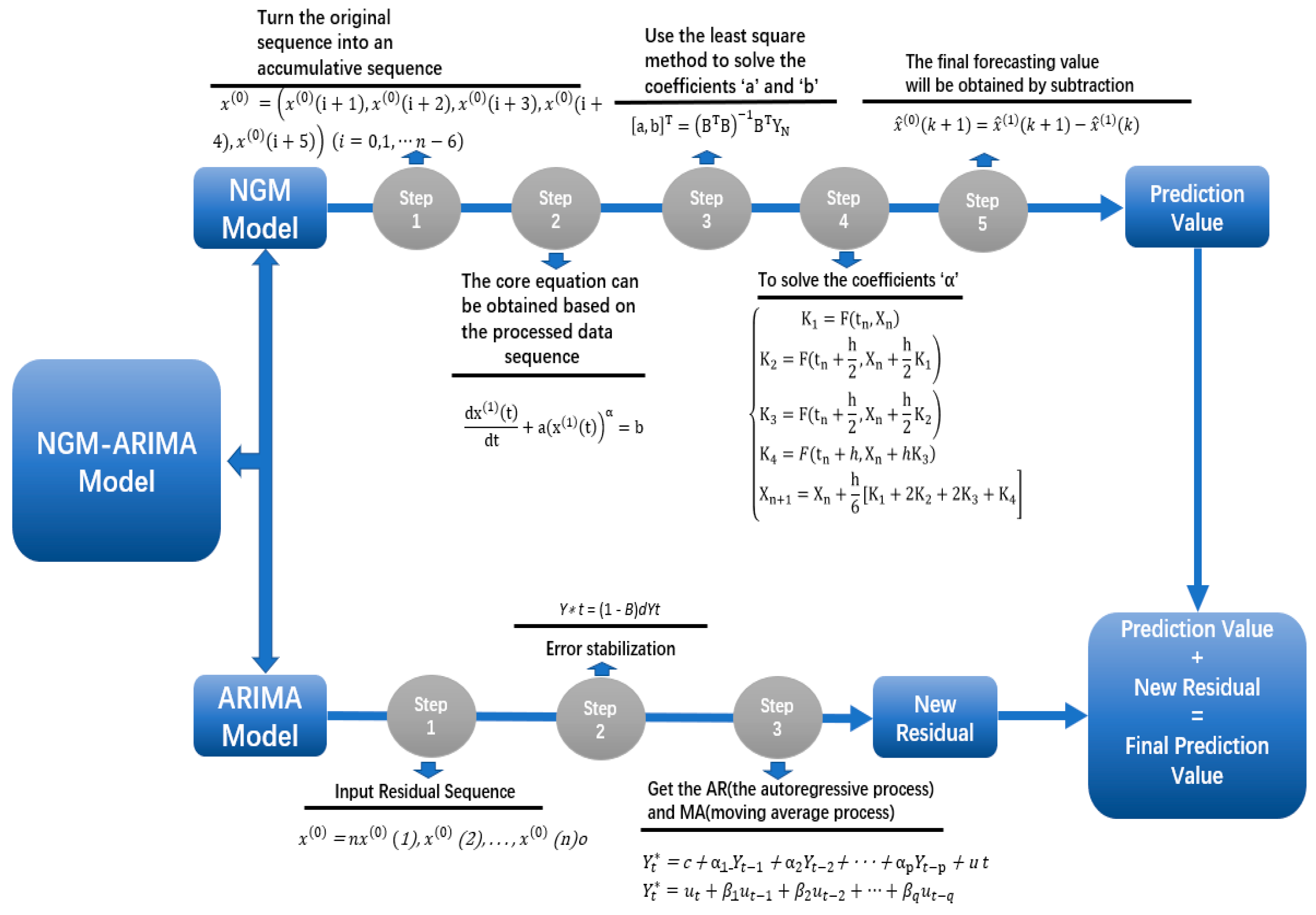
2.1.3. NGM-ARIMA Prediction Model

NGM-ARIMA model combines the NGM and ARIMA models. It has the combined advantages of linear and nonlinear models without the disadvantages of linear and nonlinear models. The ARIMA model has the advantage of simple modeling and high prediction accuracy, but it has high data stability requirements and it cannot capture the nonlinear relation of data, while NGM model can capture the nonlinear relation and has better adaptability in data processing. So, the predicted data still have high accuracy when there is a large variation in raw data.

In terms of model innovation, the NGM-ARIMA model proposed in this study is based on the new principle of “error correction + secondary modeling”. First of all, under the guidance of the error correction principle, the NGM-ARIMA model puts the initial error predicted by NGM into the input variables of the ARIMA model. This is expected to stabilize the error processing and make the final fitting curve closer to the reality. Second, guided by the principle of secondary modeling, NGM-ARIMA model chooses two kinds of time series models, and combines them in the link. The connection between the models has a certain replicable value in the combination model. Moreover, this combination can bring the advantages of the two models into play and avoid the corresponding defects. The principle of quadratic modeling is expected to make the best of the prediction process through two models.

The operation steps of the NGM-ARIMA model can be roughly divided into three steps: step 1 is to combine the raw data with the results predicted by the NGM model and obtain the residual; step 2 is to use the ARIMA model to analyze the residual and obtain the new residual through calculation; step 3 is to add the prediction value obtained from the NGM model with the new residual obtained from the ARIMA model to get the final prediction value of the NGM-ARIMA model. The specific steps are shown in Figure 1.

2.1.4. Characteristics and Limitations of Each Model

On the basis of NGM and ARIMA single models, a new combined NGM-ARIMA model is constructed according to the principle of “secondary modeling + error correction”. Among them, the NGM model is to predict the initial data sequence, while the ARIMA model is to correct the error again. This modeling idea and process of the composite model brings the following characteristics. First of all, the model only forecasts according to the historical change track of the data sequence itself. In other words, the application object of the model is only single factor time series data. Secondly, the model constructed in this study is a combination of prediction steps after superposition. Compared with the traditional improvement of the internal coefficient, this improvement between the models has a wide range of application value. As long as the latter model has the effect of stable error, the two models can be combined.

Everything has its pros and cons. The above two features not only provide the core of model construction, but also bring corresponding limitations. Since the two basic models of the composite model are all time series models, the composite model constructed in this study cannot consider the influence of other external multiple factors on the predicted data. This defect leads to the following limitations: the model constructed in this paper can only predict the data with its own historical trend but cannot measure the impact of other external factors on the data itself. Although the multifactor prediction model can fully consider the influence of all aspects, there is also the problem of error accumulation of all factors [36]. In general, the limitation of the model proposed in this study is that it cannot accurately measure the data affected by multiple factors. However, it has a good accuracy in predicting the data that are obviously affected by the historical laws.

2.2. Data Source

Considering the reliability and acquirability of research data, the data used for the research are from BP energy statistical yearbook [1], and 1998–2016 South Africa’s energy consumption has been selected as raw data to predict the South Africa’s energy consumption in 2017–2030.

3. Empirical Results and Discussion

3.1. Operation Process of the Three Models

In this part, the operation process of the ARIMA, NGM and NGM-ARIMA models will be divided into fitting and forecasting. The fitting part is to predict the South Africa’s energy consumption in 1998–2016 and compare with the raw data from the same period, and the purpose is to inspect the accuracy of these three prediction models. The MAPE formula used during the operation process is to compare the tools of raw data and fitting data accuracy so as to discover whether these three models are suitable for the research. The forecasting part is to predict the South Africa’s energy consumption in 2017–2030, and the results will be South Africa’s energy consumption in the next 14 years.

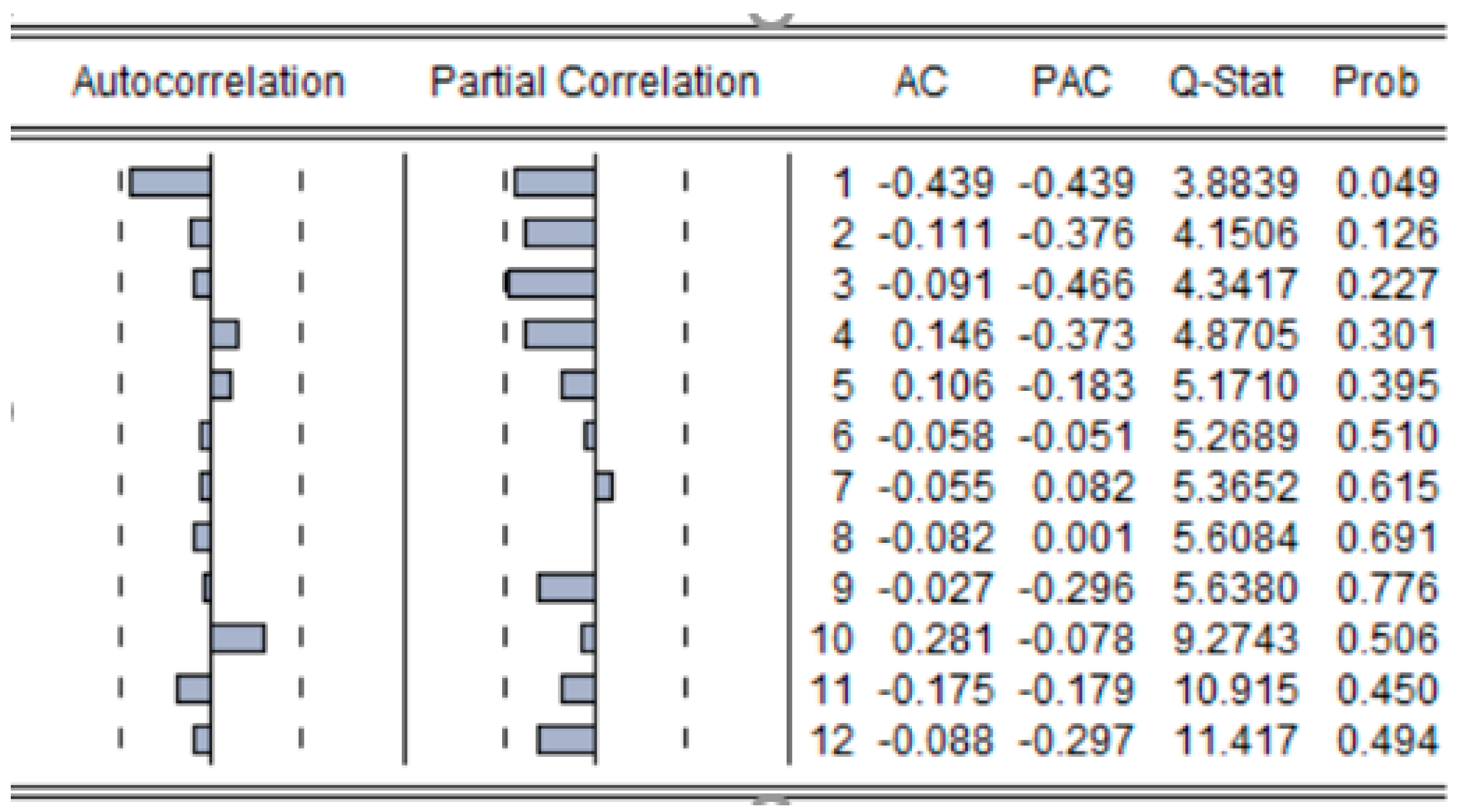
3.1.1. ARIMA Model Fitting Process

The prediction of the ARIMA model is classified into following several steps:

Step 1: Apply unit root test to raw data. The unit root test is used to make the prediction data stationary through a differential tool, and the differential order is the d value in ARIMA (p, d, q) equation.

Table 1. The resulting unit root test values after second-order difference.

Augmented Dickey–Fuller	Confidence Level	t-Statistic	Probability *
Test statistic		3.639257	0.0665
Test critical values	1% level	4.886426
	5% level	3.828975
	10% level	3.362984

shows the result after second-order difference. As shown in the table, the t-value is between 5% and 10%, and the p-value is 0.0665 (<0.1), which means that the sequence tends to stationary under 90% confidence, therefore, d = 2.

Step 2: After determining that d = 2, the p and q values can be obtained through autocorrelation coefficient. Figure 2 is the correlation coefficient chart obtained after second-order difference. It can be seen from the chart that the partial correlation coefficient chart tends to stationary after fifth-order difference and the autocorrelation coefficient chart tends to stationary after first-order difference, therefore, it can be obtained that p = 5, q = 1.

After determining that ARIMA (p, d, q) is after ARIMA (5, 2, 1), we used SPSS software to apply the next operation to the model; the parameter values obtained are shown in

Table 2. Model Statistics.

Model	Number of Predictors	Model Fit Statistics	Number of Outliers
		Stationary R2
ARIMA (5,2,1)	1	0.523	0

. It can be seen from Table 2 that the stationary R²-value is 0.523, which conforms to the goodness test standard.

The final fitting results of 1998–2016 obtained through using ARIMA (5, 2, 1) are shown in Figure 3, and the difference between fitting value and actual value can be clearly seen in this figure.

As shown in Figure 3, it can be seen from the variation trend of raw data and ARIMA prediction data that though there is slight difference between the raw data and prediction value in 2003 and 2004, the overall variation trend is basically consistent. In addition, the fitting data show that, except for the accuracy in 2003 and 2004 being 92%, the accuracies of other years are all higher than 95%, which also means that ARIMA (5, 2, 1) is applicable to the study.

3.1.2. NGM Model Fitting Process

First, we substituted the power coefficient into the operation formula of NGM in Section 2, which was then calculated using MATLAB software; the obtained power coefficient of nonlinear grey model is shown in

Table 3. The power coefficients of the NGM model.

Year	2002	2003	2004	2005	2006	2007	2008	2009
Power coefficient	1	1	1	1	0.001	0.001	0.571	1
Year	2010	2011	2012	2013	2014	2015	2016
Power coefficient	1	1	1	1	0.001	0.934	1

.

Based on the power coefficients in Table 3, and using MATLAB software(version 9.3, MathWorks, Natick, Massachusetts, USA), the final South African energy consumption predicted by NGM model was obtained, as shown in Figure 4.

As shown in Figure 4, it can be seen that the variation trend of raw data and NGM prediction data during 1998–2016 is similar, with the degrees of fitting in 2005–2007 and 2011–2014 reaching 100%. The fitting data show that the accuracy of data fitting by NGM model is high, which also indicates that NGM model is applicable to the research.

3.1.3. NGM-ARIMA Model Fitting Process

The NGM-ARIMA combined prediction model uses a linear model to correct the data residual value predicted by a nonlinear model.

First, we subtracted the NGM prediction value and primary energy consumption to obtain the residual.

Then, we used the ARIMA model to apply the unit root test to residual values, discovering that data sequence was stationary after first-order difference during inspection process; therefore, d = 1.

After determining the d value, we could obtain the p value and q value through analyzing the autocorrelation coefficient and partial correlation coefficient in the correlation coefficient figure. After several attempts, we determined that p = 3, q = 5. Therefore, ARIMA (p, d, q) is ARIMA (3, 1, 5).

We substituted the ARIMA (3, 1, 5) into SPSS software, and the result obtained was the error of NGM. Then, we combined the result with primary energy consumption; the obtained data are South Africa’s energy consumption predicted by NGM-ARIMA model. The specific prediction data are shown in the figure below:

As shown in Figure 5, if we compare the primary energy consumption in 1998–2016 with the prediction data by NGM-ARIMA, we can see that the trendlines of two groups of data are highly similar. Through analyzing the fitting data, we can discover that the fitting by using NGM-ARIMA model is as high as 98%, in which the fitted values in 2001 and 2007 are 100%. It also indicates that the data accuracy obtained through using linear and nonlinear combined model is higher than that of using single model.

3.2. Model Goodness Inspection

In this part, the prediction results obtained by ARIMA, NGM and NGM-ARIMA models will be evaluated by three different statistical indicators, to better test the goodness of fit. These indicators are mean absolute percent error (MAPE), mean squared error (MSE) and mean squared percent error (MSPE). The calculation formulas of these indicators are as follows:

$$\mathrm{MAPE}={\displaystyle {\displaystyle \sum }_{i=1}^n}\left|\frac{y_i-x_i}{x_i}\right|\times \frac{100}{n}$$

(14)

$$\mathrm{MSE}=\frac{1}{n}{\displaystyle {\displaystyle \sum }_{i=1}^n}{\left(y_i-x_i\right)}^2$$

(15)

$$\mathrm{MSPE}=\frac{1}{n}\sqrt{{\displaystyle {\displaystyle \sum }_{i=1}^n}{\left[\frac{y_i-x_i}{x_i}\right]}^2}$$

(16)

where y_i is the prediction value, x_i is the actual value and n is the sample size [37].

Table 4. The error values of each model.

Year	MAPE			MSPE			MSE
	ARIMA	NGM	NGM-ARIMA	ARIMA	NGM	NGM-ARIMA	ARIMA	NGM	NGM-ARIMA
1998	0.0000	0.0000	0.0000	0.0000	0.0000	0.0000	1.0000	1.0000	1.0000
1999	0.0000	0.0140	0.0066	0.0000	0.0002	0.0000	1.0000	0.9997	0.9999
2000	0.0262	0.0126	0.0183	0.0007	0.0002	0.0003	0.9995	0.9998	0.9996
2001	0.0024	0.0312	0.0021	0.0000	0.0010	0.0000	1.0000	0.9994	1.0000
2002	0.0300	0.0819	0.0099	0.0009	0.0067	0.0001	0.9994	0.9983	0.9998
2003	0.0853	0.0151	0.0391	0.0073	0.0002	0.0015	0.9984	0.9997	0.9993
2004	0.0847	0.0536	0.0072	0.0072	0.0029	0.0001	0.9985	0.9991	0.9999
2005	0.0479	0.0148	0.0218	0.0023	0.0002	0.0005	0.9991	0.9997	0.9996
2006	0.0294	0.0052	0.0345	0.0009	0.0000	0.0012	0.9995	0.9999	0.9994
2007	0.0114	0.0000	0.0047	0.0001	0.0000	0.0000	0.9998	1.0000	0.9999
2008	0.0419	0.0604	0.0078	0.0018	0.0036	0.0001	0.9993	0.9990	0.9999
2009	0.0333	0.0475	0.0396	0.0011	0.0023	0.0016	0.9995	0.9992	0.9994
2010	0.0191	0.0436	0.0228	0.0004	0.0019	0.0005	0.9997	0.9993	0.9996
2011	0.0271	0.0193	0.0243	0.0007	0.0004	0.0006	0.9996	0.9997	0.9996
2012	0.0465	0.0052	0.0227	0.0022	0.0000	0.0005	0.9992	0.9999	0.9996
2013	0.0067	0.0022	0.0054	0.0000	0.0000	0.0000	0.9999	1.0000	0.9999
2014	0.0067	0.0006	0.0051	0.0000	0.0000	0.0000	0.9999	1.0000	0.9999
2015	0.0311	0.0527	0.0122	0.0010	0.0028	0.0001	0.9995	0.9991	0.9998
2016	0.0071	0.0443	0.0527	0.0001	0.0020	0.0028	0.9999	0.9993	0.9991
Average	0.0283	0.0265	0.0177	0.0086	0.0082	0.0053	0.9995	0.9995	0.9997

shows the three error values of these three models obtained through the above formulas, in which, the last line of the table exhibits the mean value of each error, which can also be used as the final measurement results of the error term.

Figure 6 is drawn by using the result of MAPE in Table 4 and it clearly shows the accuracy of data in 1998–2016 predicted by using ARIMA, NGM and NGM-ARIMA model. Just as shown in the figure, though the accuracy of 2003–2004 prediction data by ARIMA model and 2002 by NGM model is slightly lower than that of other years, the mean value of accuracy predicted by these three models is higher than 97%.

Through the measurement tools for prediction accuracy of the above models, we can see that: (1) The MAPE of these three models is less than 3%; in which, the MAPEs of ARIMA model, NGM model and NGM-ARIMA model are 2.827%, 2.655% and 1.772%, respectively. (2) The spider web chart indicates that, except for a mark of 92% reached by ARIMA model accuracy in 2003 and 2004 and by NGM model in 2002, the prediction accuracy of other years exceeded 95%. Based on the two measurement results above, we can make sure that the three models are applicable to the research, that the predicted data credibility is high, and the prediction result is of high reference value.

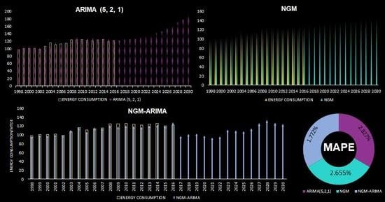
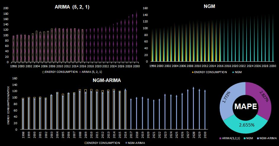
3.3. Prediction Results and Discussion

Table 5. Predictive values of different models.

YEAR	ARIMA (5, 2, 1)	NGM	NGM-ARIMA
2017	121.6615	128.9256	97.7957
2018	124.5612	130.1407	102.4731
2019	125.1492	131.3387	103.3278
2020	126.6525	132.5208	98.5698
2021	128.3105	133.6881	93.6602
2022	133.1727	134.8415	96.3183
2023	136.0278	135.982	112.6159
2024	142.0273	137.1102	110.6475
2025	145.8276	138.2269	108.5081
2026	153.6211	139.3328	115.2856
2027	160.2464	140.4284	127.6118
2028	169.8985	141.5143	134.5952
2029	178.2913	142.5909	128.2806
2030	190.0362	143.6588	125.6522

shows South Africa’s energy consumption in 2017–2030 predicted by using ARIMA, NGM and NGM-ARIMA models. Figure 7 is the variation trend chart of consumption drawn according to the prediction result of Table 5, where the change of South Africa’s energy consumption can be seen more clearly.

From Figure 7, we can see that the degree of fitting of three models is very high in previous prediction and primary energy consumption. In addition, South Africa’s energy consumption in 2017–2030 predicted by these three models presents stable growth tendency.

Specific to the prediction result of the research, we will discuss the following two aspects:

Firstly, from the analysis of prediction model, the energy consumption tendency predicted by the two models is consistent and the error is less than 3% after the detection of MAPE. It also has proved that the prediction result has high credibility. However, since these three models are time sequence models, the impact of other factors to South Africa’s energy consumption have not been considered during modeling process, it may have the incomplete analysis of energy consumption.

Secondly, from the analysis of prediction result, South Africa’s energy consumption in 2030 will be increased by 27.19 Mtoe than that in 2016. In addition, it can be seen clearly from Figure 7 that South Africa’s energy consumption will keep increasing for a long time in the future. Under the circumstance that the energy reserve is unchanged, it will undoubtedly cause imbalanced energy supply and demand; Therefore, South Africa should guarantee the energy supply while increasing the energy consumption.

4. Conclusions

This paper aimed to accurately predict the South Africa’s energy consumption in 2017–2030 by using a linear model (ARIMA), a nonlinear model (NGM) and a linear–nonlinear combined model (NGM-ARIMA) in time sequence modeling. The research results show that the MAPEs of each model are 2.827%, 2.655% and 1.772%, respectively, which indicates that the three models are applicable to the research. The accuracy predicted by the NGM-ARIMA model is the highest, and the prediction result is the closest to the actual energy consumption. This means that the research could provide scientific and reliable data support for the prediction of South Africa’s energy.

By calculating the prediction result, we can see that the South Africa’s energy consumption in 2017–2030 will keep increasing with about 7.49% growth rate and it will be increased by 17.8% in 2030 compared to that in 2016. In other words, South Africa’s energy consumption in the next 14 years will still exhibit sustainable and stable growth; this result is consistent with the rapid economic development of South Africa [38].

This prediction result means that in the future, the South African government needs to pay more attention to the change of energy supply and demand so as to guarantee the balance between energy supply and demand and thus lay a foundation for promoting South Africa’s rapid and stable economic development and people’s living standard. In addition, the prediction technique of the research will be of reference significance to the research of energy consumption in other African countries and regions.

References

1. Dudley, B. Statistical Review of World Energy; BP Statistical Review: London, UK, 2018. [Google Scholar]
2. Ebohon, O.J. Energy, economic growth and causality in developing countries: A case study of Tanzania and Nigeria. Energy Policy 2007, 24, 447–453. [Google Scholar] [CrossRef]
3. Gessner, U.; Knauer, K.; Machwitz, M.; Dech, S.; Kuenzer, C. Impacts of Socio-economic Development and Urbanization on Natural Resources-Case Studies from Africa. In Proceedings of the Geoscience and Remote Sensing Symposium, Beijing, China, 10–15 July 2016. [Google Scholar]
4. Oyedepo, S.O. On energy for sustainable development in Nigeria. Renew. Sustain. Energy Rev. 2012, 16, 2583–2598. [Google Scholar] [CrossRef]
5. Adom, P.K.; Bekoe, W. Conditional dynamic forecast of electrical energy consumption requirements in Ghana by 2020: A comparison of ARDL and PAM. Energy 2012, 44, 367–380. [Google Scholar] [CrossRef]
6. Bazilian, M.; Nussbaumer, P.; Rogner, H.H.; Brew-Hammond, A.; Foster, V.; Pachauri, S.; Williams, E.; Howells, M.; Niyongabo, P.; Musaba, L.; et al. Energy access scenarios to 2030 for the power sector in sub-Saharan Africa. Util. Policy 2012, 20, 1–16. [Google Scholar] [CrossRef] [Green Version]
7. Mentis, D.; Hermann, S.; Howells, M.; Welsch, M.; Siyal, S.H. Assessing the technical wind energy potential in Africa a GIS-based approach. Renew. Energy 2015, 83, 110–125. [Google Scholar] [CrossRef]
8. Sigauke, C.; Chikobvu, D. Prediction of daily peak electricity demand in South Africa using volatility forecasting models. Energy Econ. 2011, 33, 882–888. [Google Scholar] [CrossRef]
9. Thopil, G.A.; Pouris, A. A 20 year forecast of water usage in electricity generation for South Africa amidst water scarce conditions. Renew. Sustain. Energy Rev. 2016, 62, 1106–1121. [Google Scholar] [CrossRef] [Green Version]
10. Tsikata, M.; Sebitosi, A.B. Struggling to wean a society away from a century-old legacy of coal based power: Challenges and possibilities for South African Electric supply future. Energy 2010, 35, 1281–1288. [Google Scholar] [CrossRef]
11. Ayodele, T.R.; Jimoh, A.A.; Munda, J.L.; Agee, J.T. A Statistical Analysis of Wind Distribution and Wind Power Potential in the Coastal Region of South Africa. Int. J. Green Energ. 2013, 10, 814–834. [Google Scholar] [CrossRef]
12. Walwyn, D.R.; Brent, A.C. Renewable energy gathers steam in South Africa. Renew. Sustain. Energy Rev. 2015, 41, 390–401. [Google Scholar] [CrossRef] [Green Version]
13. Malondkar, A.; Corizzo, R.; Kiringa, I.; Ceci, M.; Japkowicz, N. Spark-GHSOM: Growing Hierarchical Self-Organizing Map for large scale mixed attribute datasets. Inf. Sci. 2019, 496, 572–591. [Google Scholar] [CrossRef]
14. Ayodele, T.R.; Ogunjuyigbe, A.S.O. Prediction of wind speed for the estimation of wind turbine power output from site climatological data using artificial neural network. Int. J. Ambient. Energy 2015, 38, 29–36. [Google Scholar] [CrossRef]
15. Sotomane, C.; Asker, L.; Boström, H.; Massingue, V. Short-term Forecasting of Electricity Consumption in Maputo. In Proceedings of the International Conference on Advances in ICT for Emerging Regions. (ICTer), Colombo, Sri Lanka, 11–15 December 2013; pp. 132–136. [Google Scholar]
16. Inglesi, R. Aggregate electricity demand in South Africa: Conditional forecasts to 2030. Appl. Energy 2010, 87, 197–204. [Google Scholar] [CrossRef] [Green Version]
17. Ahjum, F.; Merven, B.; Cullis, J.; Goldstein, G.; DeLaquil, P.; Stone, A. Development of a national water-energy system model with emphasis on the power sector for south africa. Environ. Prog. Sustain. Energy 2018, 37, 132–147. [Google Scholar] [CrossRef]
18. Fadare, D.A. Modelling of solar energy potential in Nigeria using an artificial neural network model. Appl. Energy 2009, 86, 1410–1422. [Google Scholar] [CrossRef]
19. Bessa, R.J.; Trindade, A.; Miranda, V. Spatial-temporal solar power forecasting for smart grids. IEEE Trans. Ind. Inform. 2014, 11, 232–241. [Google Scholar] [CrossRef]
20. Ceci, M.; Corizzo, R.; Malerba, D.; Rashkovska, A. Spatial autocorrelation and entropy for renewable energy forecasting. Data Min. Knowl. Discov. 2019, 33, 698–729. [Google Scholar] [CrossRef]
21. Abdel-Nasser, M.; Mahmoud, K. Accurate photovoltaic power forecasting models using deep LSTM-RNN. Neural Comput. Appl. 2019, 31, 2727–2740. [Google Scholar] [CrossRef]
22. Wang, Q.; Li, S.; Li, R. China’s Dependency on Foreign Oil Will Exceed 80% by 2030: Developing a Novel NMGM-ARIMA to Forecast China’s Foreign Oil Dependence from Two Dimensions. Energy 2018, 163, 151–167. [Google Scholar] [CrossRef]
23. Wang, Q.; Li, S.; Li, R. Forecasting Energy Demand in China and India: Using Single-linear, Hybrid-linear, and Non-linear Time Series Forecast Techniques. Energy 2018, 161, 821–831. [Google Scholar] [CrossRef]
24. Bartholomew, D.J. Time Series Analysis Forecasting and Control. J. Oper. Res. Soc. 1971, 22, 199–201. [Google Scholar] [CrossRef]
25. Ramakrishna, G.; Kumari, R.V. Arima Model for Forecasting of Rice Production in India by Using Sas. Siam J. Appl. Math. 2018, 6, 67–72. [Google Scholar]
26. Sen, P.; Roy, M.; Pal, P. Application of ARIMA for forecasting energy consumption and GHG emission: A case study of an Indian pig iron manufacturing organization. Energy 2016, 116, 1031–1038. [Google Scholar] [CrossRef]
27. Zhao, H.; Guo, S. An optimized grey model for annual power load forecasting. Energy 2016, 107, 272–286. [Google Scholar] [CrossRef]
28. Li, S.; Li, R. Comparison of forecasting energy consumption in Shandong, China Using the ARIMA model, GM model, and ARIMA-GM model. Sustainability 2017, 9, 1181. [Google Scholar]
29. Yuan, C.; Liu, S.; Fang, Z. Comparison of China’s primary energy consumption forecasting by using ARIMA (the autoregressive integrated moving average) model and GM (1, 1) model. Energy 2016, 100, 384–390. [Google Scholar] [CrossRef]
30. Zhang, Q.; Li, Z.; Snowling, S.; Siam, A.; El-Dakhakhni, W. Predictive models for wastewater flow forecasting based on time series analysis and artificial neural network. Water Sci. Technol. 2019, 80, 243–253. [Google Scholar] [CrossRef]
31. Lu, B.; Zhao, S.; Tian, Y.; Yang, Y.; Li, B.; Chen, X. Mid-long term electricity consumption forecasting based on improved NGM (1, 1, k) gray model. Power Syst. Prot. Control 2015, 43, 98–103. [Google Scholar]
32. Du, Y.; Liang, W.; Wang, H.; Hua, W. Coal consumption forecast in anhui province-based on GM (1, 1). J. Tonghua Normal Univ. 2016, 37, 25–26. [Google Scholar]
33. Guo, X.; Liu, S.; Wu, L.; Tang, L. A grey NGM (1, 1, k) self-memory coupling prediction model for energy consumption prediction. Sci. World J. 2014, 2014, 327. [Google Scholar] [CrossRef]
34. Wang, Z.X. Nonlinear Grey Prediction Model with Convolution Integral NGMC (1, n) and Its Application to the Forecasting of China’s Industrial SO2 Emissions. J. Appl. Math. 2014, 2014, 174–178. [Google Scholar]
35. Ren, S.; Chan, H.L.; Ram, P. A Comparative Study on Fashion Demand Forecasting Models with Multiple Sources of Uncertainty. Ann. Oper. Res. 2016, 257, 1–21. [Google Scholar] [CrossRef]
36. Boyd, G.; Na, D.; Li, Z.; Snowling, S.; Zhang, Q.; Zhou, P. Influent Forecasting for Wastewater Treatment Plants in North America. Sustainability 2019, 11, 1764. [Google Scholar] [CrossRef] [Green Version]
37. Khair, U.; Fahmi, H.; Al Hakim, S.; Rahim, R. Forecasting Error Calculation with Mean Absolute Deviation and Mean Absolute Percentage Error. J. Phys. Conf. Ser. IOP Publ. 2017, 930, 012002. [Google Scholar] [CrossRef]
38. Odhiambo, N.M. Savings and economic growth in South Africa: A multivariate causality test. J. Policy Model. 2009, 31, 708–718. [Google Scholar] [CrossRef]
Figure 1. The origin and formation of the combined nonlinear grey model–autoregressive integrated moving average (NGM-ARIMA) model.
Energies 13 00010 g001
Figure 2. The stationary sequence correlation plot.
Energies 13 00010 g002
Figure 3. The prediction of ARIMA model.
Energies 13 00010 g003
Figure 4. The prediction of NGM model.
Energies 13 00010 g004
Figure 5. The prediction of NGM-ARIMA model.
Energies 13 00010 g005
Figure 6. The accuracy of each model in each year.
Energies 13 00010 g006
Figure 7. The final predictions of ARIMA model, NGM model and NGM-ARIMA model.
Energies 13 00010 g007