Article

Reactive Power Capability Model of Wind Power Plant Using Aggregated Wind Power Collection System

1
Department of Wind Energy, Technical University of Denmark, 4000 Roskilde, Denmark
2
Energy Systems Engineering Department, Izmir Institute of Technology, Urla, 35430 Izmir, Turkey
*
Author to whom correspondence should be addressed.
Energies 2019, 12(9), 1607; https://doi.org/10.3390/en12091607
Submission received: 20 March 2019 / Revised: 14 April 2019 / Accepted: 23 April 2019 / Published: 27 April 2019
(This article belongs to the Special Issue Modeling of Wind Turbines and Wind Farms)

Abstract

:
This article presents the development of a reactive power capability model for a wind power plant (WPP) based on an aggregated wind power collection system. The voltage and active power dependent reactive power capability are thus calculated by using aggregated WPP collection system parameters and considering losses in the WPP collection system. The strength of this proposed reactive power capability model is that it not only requires less parameters and substantially less computational time compared to typical detailed models of WPPs, but it also provides an accurate estimation of the available reactive power. The proposed model is based on a set of analytical equations which represent converter voltage and current limitations. Aggregated impedance and susceptance of the WPP collection system are also included in the analytical equations, thereby incorporating losses in the collection system in the WPP reactive power capability calculation. The proposed WPP reactive power capability model is compared to available methodologies from literature and for different WPP topologies, namely, Horns Rev 2 WPP and Burbo Bank WPP. Performance of the proposed model is assessed and discussed by means of simulations of various case studies demonstrating that the error between the calculated reactive power using the proposed model and the detailed model is below 4% as compared to an 11% error in the available method from literature. The efficacy of the proposed method is further exemplified through an application of the proposed method in power system integration studies. The article provides new insights and better understanding of the WPPs’ limits to deliver reactive power support that can be used for power system stability assessment, particularly long-term voltage stability.

1. Introduction

Growing concerns for climate change, energy security, increasing fuel prices for non-renewable generation sources, price reduction for renewable sources like wind and solar power are driving power systems to have a larger share of renewables all over the world. Due to large onshore and offshore developments, wind power is set to become the leading source of electricity in Europe after 2030 [1]. Around 52.6 GW of wind power capacity was installed globally in 2017, increasing the net installed capacity to 539.6 GW [1]. Increase in the share of renewables is also phasing out the conventional generations like coal based power plants, which brings many new challenges in operation and stability of the power system. Some of these challenges include a decrease in inertia, active and reactive power fluctuations, network congestion, etc. This article deals with reactive power reserve and support from wind power plants (WPP). The reactive power reserves conventionally provided by exciter of synchronous generator reduces when replaced by WPPs. This can cause voltage stability issues. This issue is further pronounced in weak grids where WPPs are connected to the grid through long lines. The need for analysis of reactive power support from WPP is especially essential when the grid is in a stressed condition. However, integration of hundreds of WPPs in large power system analysis is very complex and computationally intensive. Therefore, simplified representations of WPPs accurate enough to reflect capabilities and limitations of the converter based wind turbines (WTs) are required to analyze future power systems.
In power system stability analysis, long-term voltage stability is defined as a slow phenomenon involving slow acting equipment like tap-changing transformers, thermostatically controlled loads, generator limiters etc., such that the network is unable to provide adequate reactive power support (at least at certain nodes or areas in the power system) [2,3]. Traditionally, realistic representations of synchronous generators along with automatic voltage regulators have been used to model the capabilities and limits of reactive power resources in long-term voltage stability studies [2]. A similar reactive power resource model for WPPs needs to be developed for future power systems dominated by converter connected power generations. In this article, WPP reactive power capability is developed for an accurate representation of maximum reactive power generation and absorption capability of IEC 61400-27-1 [4] Type 4 WT (full rated converter based WT) based WPPs.
Several studies have been carried out over the years, where WPP reactive power capability has been used for power system analyses. Reactive power capability has been used to determine the voltage dependent reactive current limitation for modelling of WT by Bech [5] and Sørensen et al. [6]. In power system operation studies, reactive power capabilities of WPPs have been used for load flow studies in [7,8]. Zhang et al. have applied reactive power capability curves of IEC 61400-27-1 Type 3 (also known as doubly fed induction generator (DFIG)) WT for loss minimisation in WPP [9]. Inclusion of Type 3 WTs in optimal power flow for loss minimisation of distribution network have been investigated by Meegahapola et al. [10]. System flexibility studies have been performed by Stankovíc and Söder to determine the reactive power capability of distribution systems with distributed wind generations [11]. Network planning studies including the reactive power capability of WPPs have been done by Ugranli and Karatepe [12]. Reactive power reserve management of WPPs considering the maximum capability of WTs have been proposed by Martínez et al. [13]. Voltage control at the point of common coupling (PCC) considering reactive power capability of WPPs have been investigated by Kim et al. [14] and Karbouj et al. [15]. Reactive power capability of WPPs have also been applied for voltage stability studies. Dynamic voltage stability studies incorporating capability curves have been done by Meegahapola et al. [16]. Londero et al. [17] and Amarasekara et al. [18] have considered WT capability curves to analyze the long-term voltage stability of a power system with wind power generation. Vijayan et al. [19] have developed a voltage stability assessment method depicting that the inclusion of a WT capability curve can result in a larger power transfer margin of the system. Reactive power capability curves have also been applied for studies on ancillary services. For example, Ullah et al. have developed a generalized reactive power cost model for WPPs based on Type 4 WTs [20]. Voltage support as an ancillary service from WPPs using capability curves (for both dynamic and steady-state) have been studied by Karbouj and Rather [15].
Modelling of capability curves can be broadly categorized into: (i) WT capability curves and (ii) WPP capability curves. Lund et al. [21] have derived the steady-state capability of Type 3 WT considering rotor current, rotor voltage and stator current limitation as well as the effect of switching of coupling of DFIG stator on the capability curve. Engelhardt et al. [22] have derived capability of Type 3 WTs considering the generator and converter current limitation, losses in the machine and converter, saturation of flux, converter output voltage limitation, etc. Ullah et al. [20] have derived an analytical expression to compute reactive power capability of Type 4 WTs.
There has been limited work for representing capability curve of a WPP. Generally, there are two methods used in literature for modelling a WPP capability curve:
  • Scaled WT model: The WPP capability curve is derived by scaling up the WT capability curve with number of WTs. Kayikçi and Milanovic have used reactive power capability of WT for reactive power control of WPP, where only a single WT is modelled [23]. Konopinski et al. have modelled the reactive power capability of WPP assuming that the capability of one WT can be scaled to represent the accurate aggregate behaviour of WPP [24]. Ullah et al. have derived the reactive power capability of an aggregated WPP by scaling the output with number of wind turbines in the plant [20]. Meegahapola et al. [16,25] and Londero et al. [17] have used scaled reactive power capability of a WT for WPP representation. Meegahapola et al. [16] and Konopinski et al. [24] have developed capability curve of Type 3 based aggregated WPPs, while Ullah et al. [20] have developed it for Type 4 based aggregated WPPs.
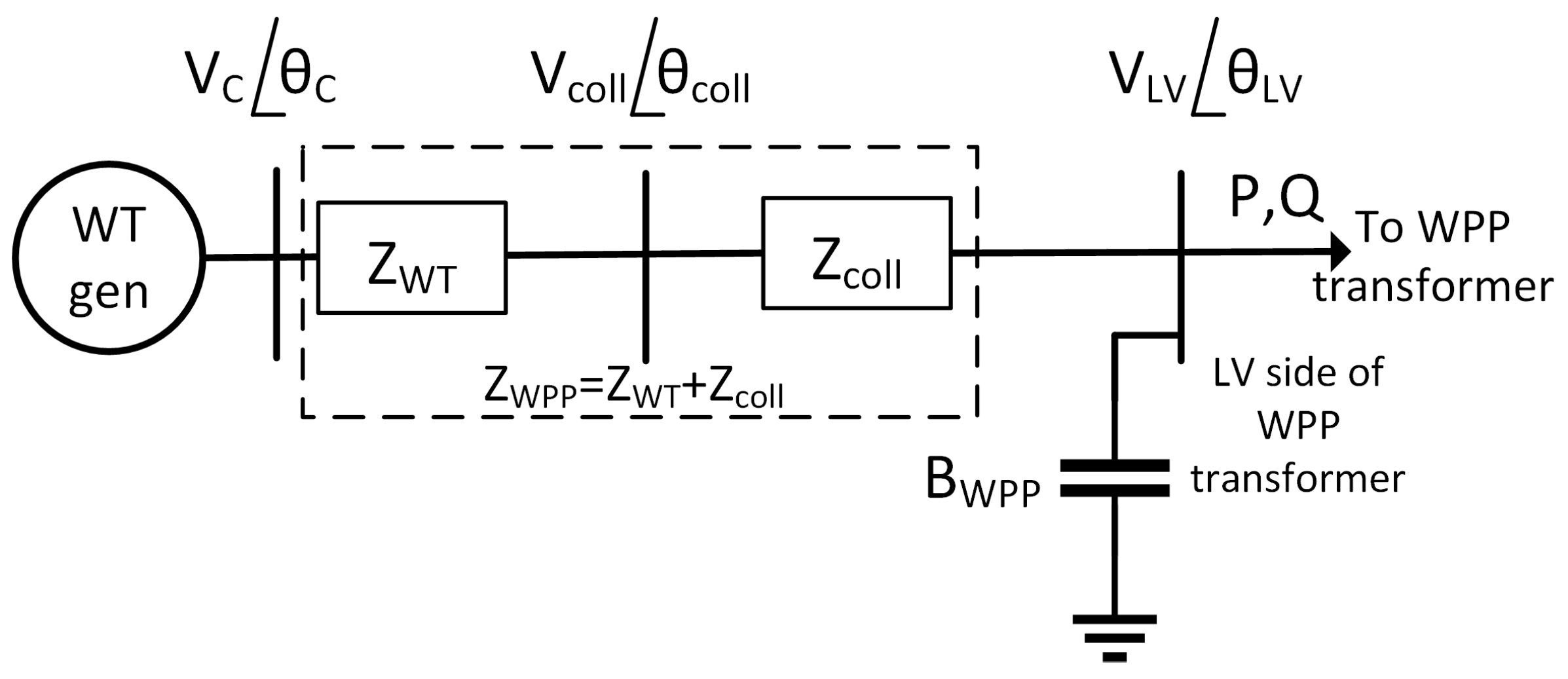
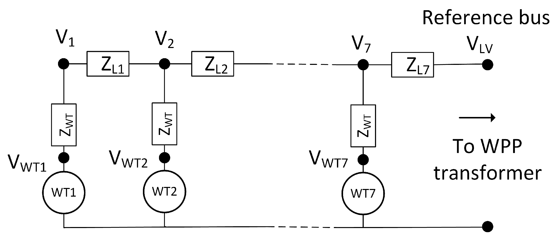
  • WPP detailed model: This involves using a detailed WPP model (including WT transformers and WPP collection system cables’ parameters). Kim et al. [26,27] have derived a reactive power capability of Type 3 based WPP based on detailed model of the WPP collection system. Karbouj and Rather [15] have modelled capability curves for Type 4 based WPPs using ABCD parameters of a detailed power collection system.
All these existing methodologies described in literature cannot be applied for simulating large power systems with numerous WPPs because of the following reasons:
  • Scaled WT models do not consider WPP collection system parameters; hence, losses in the collection system are neglected. This reduces the accuracy of the reactive power capability estimation.
  • For WPPs consisting of large number of WTs, using a detailed model of wind power collection system requires large computational time and resources. This is further worsened when system studies are performed with multiple WPPs in the network. Capability curves need to be computed in real time to utilize the full potential of WPPs in case of stressed system conditions, since reactive power capability of WPPs is dependent on active power production as well as on grid voltage conditions.
  • Detailed parameters of WPP collection systems may not be always available to system operators for estimation of reactive power reserve from WPPs.
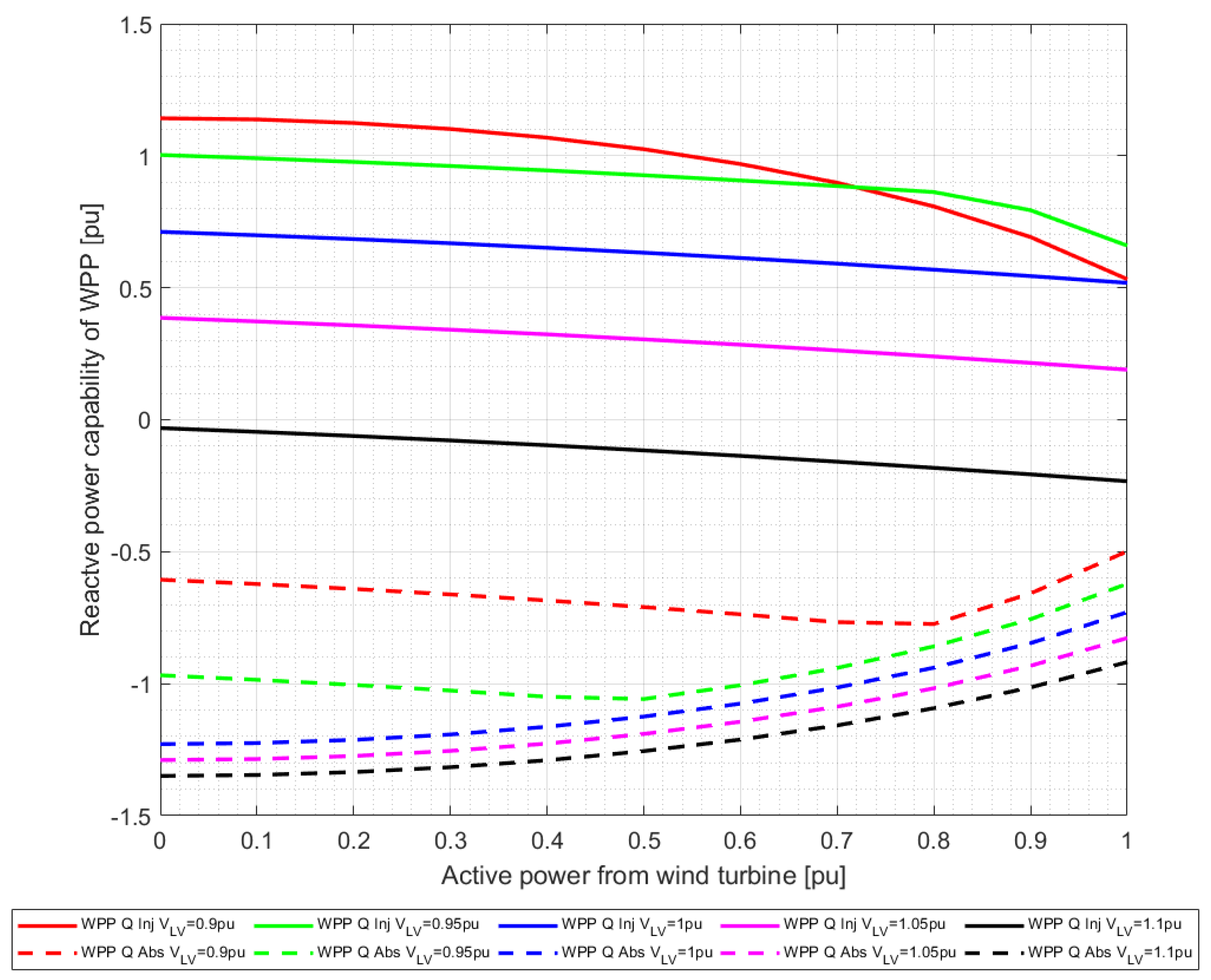
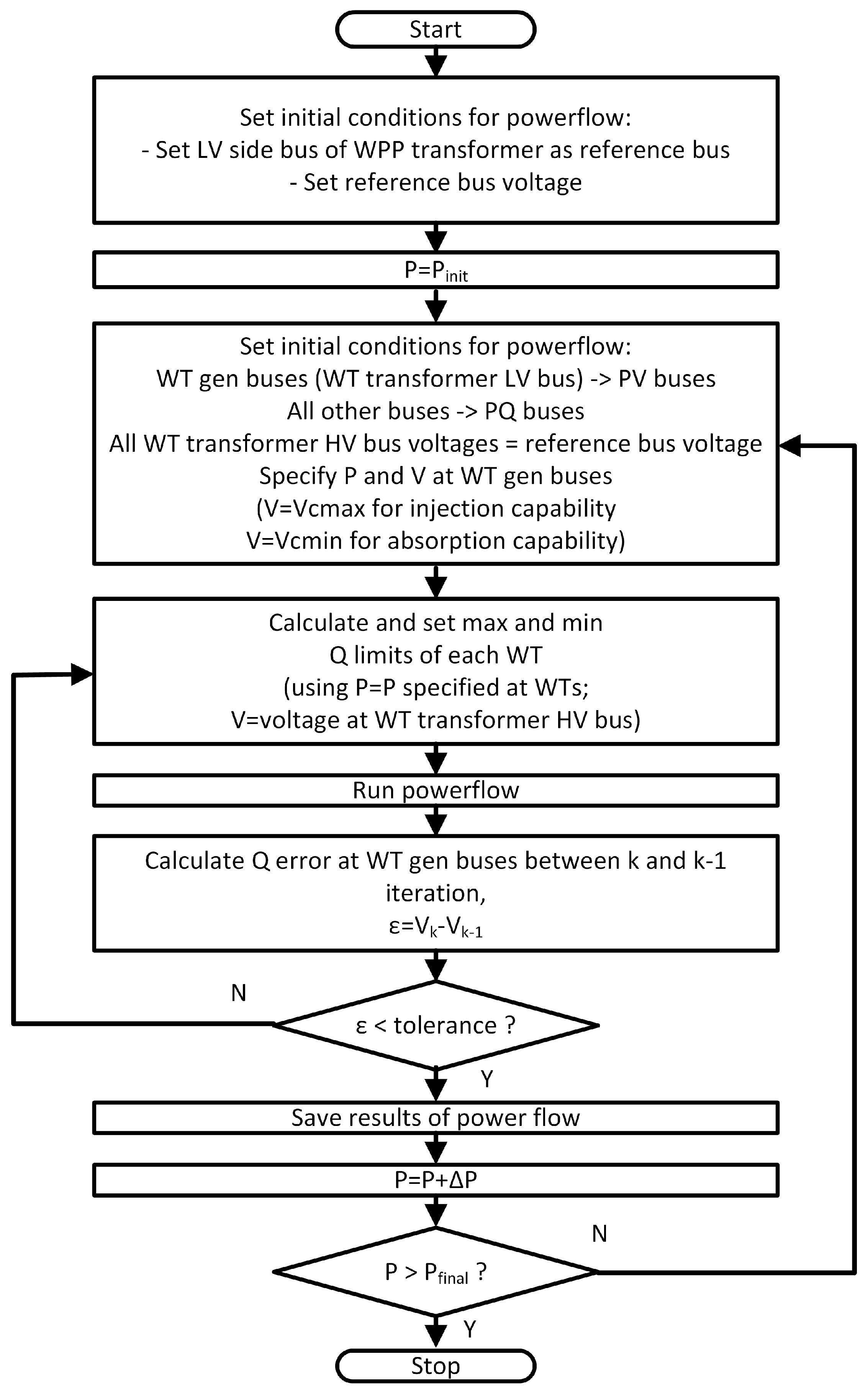
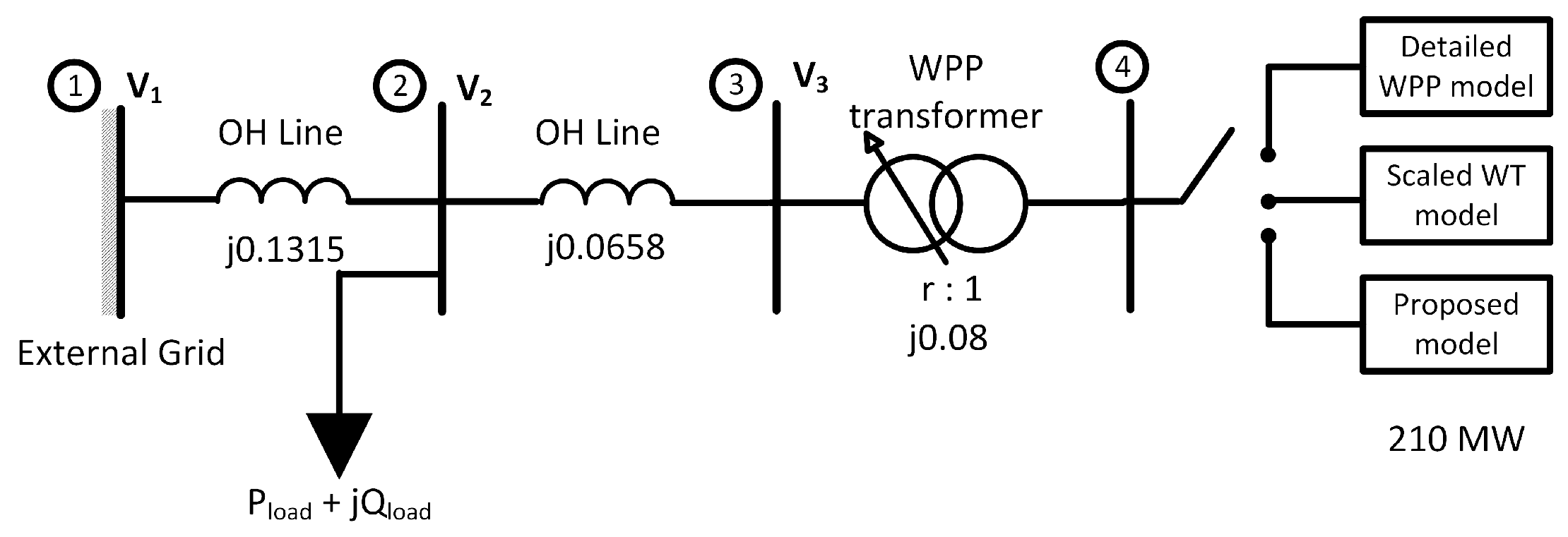
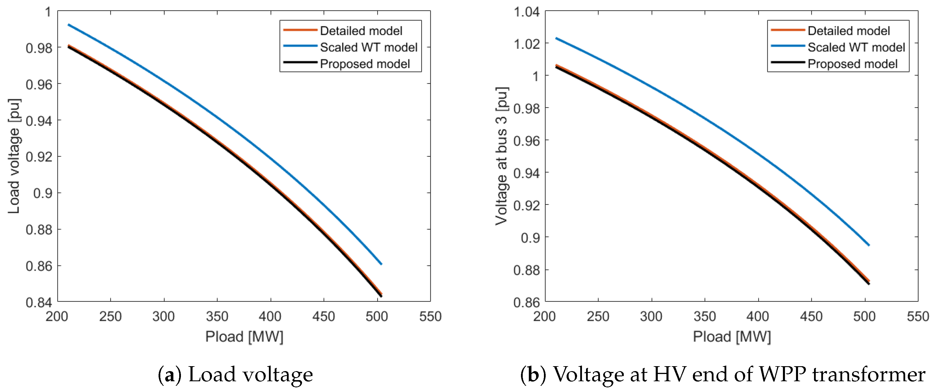
Therefore, authors have developed a new reactive power capability model in this article which estimates reactive power close to the detailed model while requiring less parameters and computation time. The objective of this article is to develop a reactive power capability model of WPP considering the WPP collection system. The developed model considers active power generation from the WPP as well as voltage dependency at the PCC. Inclusion of the collection system assures that the active and reactive power losses in the collection system are taken into account while computing WPP capability curves. Reduced the number of parameters enables fast real-time calculation of reactive power availability of any WPP. The capability curve of WPPs is dependent on various parameters such as the number of WTs, collection system configuration and length of array cables. Sensitivity studies are performed in order to realize the impact of aforementioned parameters on the WPP capability curve. The accuracy of the proposed model is compared against the WPP detailed model and scaled WT model for different simulated case studies of real WPPs. Furthermore, all these methodologies are applied on a simulated power system model to exemplify the efficacy of the proposed model.
Organisation of the article is as follows: Section 2 describes the methodology for modelling of WPP reactive power capability. In Section 3, case studies are presented and discussed to understand effects of various parameters on WPP reactive power capability. Application of the reactive power capability model for power system studies is also shown in this section. Finally, conclusive remarks are reported in Section 4.

2. Modelling

In this section firstly, the reactive power capability model of Type 4 WT is extended to include both resistance and reactance in the system. Then this model together with the aggregated WPP collection system impedance is further used to calculate WPP reactive power capability.

2.1. Extension of WT Reactive Power Capability Model

The Type 4 WT consists of a generator connected to the grid through full-scale back-to-back converters—machine side converter (MSC) and grid side converter (GSC) [28]. Schematic representation of Type 4 WT with permanent magnet synchronous generator (PMSG) is shown in Figure 1.
Back-to-back converters decouples the WT generator from the grid as well as allowing independent control of active and reactive power. Reactive power is supplied by GSC and is determined by GSC design parameters, namely, current and voltage limitations. The current limitation is due to the maximum current carrying capacity of GSC. Characteristics of power electronics set the maximum and minimum voltage limitation on GSC.
As seen in Figure 1, GSC is connected to the WT transformer through a filter and a short line. Since WT generator generates power at a low voltage level (typically 0.69 kV), the WT transformer is used to step up voltage to medium voltage level (typically 33 kV or 66 kV) to connect to the WPP collection system.
By aggregating the filter and line impedance, Figure 1 can be simplified into GSC with an equivalent impedance in series as shown in Figure 2.
In Figure 2, V C and θ C represent the converter voltage magnitude and angle, respectively. V c o l l and θ c o l l denote the voltage magnitude and angle at the WPP collection system, that is, at the high voltage (HV) side of the WT transformer. The equivalent impedance, Z W T represents impedance from GSC up to the HV side of the WT transformer. Reactive power capability is dependent on two limiting factors—converter voltage limitation and converter current limitation.

2.1.1. Converter Voltage Limitation

Ullah et al. [20] have derived converter voltage limited reactive power capability based on an analogy with the field current limit of a synchronous generator. The relation between P and Q given by Ullah et al. [20] is shown in (1).
P 2 + Q + V c o l l 2 X W T 2 = V c V c o l l X W T 2 .
Equation (1) from [20] is limited as it consists of only reactance and neglects resistance. However, in this article, WT reactive power capability model is extended for WPP including all resistance and reactance in the circuit.
The relationship between active power, reactive power, voltage and current at the HV side of the WT transformer is given by (2).
P + j Q = V c o l l θ c o l l I * ,
where
P=active power measured at HV side
Q=reactive power measured at HV side
V c o l l =voltage at HV side
θ c o l l =voltage angle at HV side
I =complex current flowing into the WPP collection system
Current flowing in the circuit of Figure 2a can be expressed as (3)
I = V C θ C V c o l l θ c o l l Z W T
where
Z W T =equivalent impedance of line, filter and WT transformer
= R W T + j X W T
V C =converter voltage magnitude
θ C =converter voltage angle
Replacing the current in (2) by (3):
P + j Q = V c o l l θ c o l l V C θ C V c o l l θ c o l l R W T + j X W T * .
Applying mathematical operation and separating real and imaginary parts, equations for active and reactive power can be written as:
P = 1 R W T 2 + X W T 2 V c o l l V C ( R W T cos θ X W T sin θ ) V c o l l 2 R W T ,
Q = 1 R W T 2 + X W T 2 V c o l l V C ( X W T cos θ + R W T sin θ ) V c o l l 2 X W T ,
where, θ = θ c o l l θ C . Rearranging (5) and (6) and squaring both sides,
P 2 ( R W T 2 + X W T 2 ) 2 + V c o l l 4 R W T 2 + 2 P ( R W T 2 + X W T 2 ) V c o l l 2 R W T = V c o l l 2 V C 2 ( R W T cos θ X W T sin θ ) 2 ,
Q 2 ( R W T 2 + X W T 2 ) 2 + V c o l l 4 X W T 2 + 2 Q ( R W T 2 + X W T 2 ) V c o l l 2 X W T = V c o l l 2 V C 2 ( X W T cos θ + R W T sin θ ) 2 .
By adding (7) and (8), applying mathematical manipulations and simplifying, (9) is obtained.
P + V c o l l 2 R W T R W T 2 + X W T 2 2 + Q + V c o l l 2 X W T R W T 2 + X W T 2 2 = V c o l l V C R W T 2 + X W T 2 2 .
Equation (9) can be rearranged and the reactive power limited by converter voltage can be written as a function of active power, converter voltage, voltage at WPP collection system and equivalent impedance as given by (10)
Q V = V c o l l V C R W T 2 + X W T 2 2 P + V c o l l 2 R W T R W T 2 + X W T 2 2 V c o l l 2 X W T R W T 2 + X W T 2 .
The maximum injection, Q V , i n j and absorption, Q V , a b s of reactive power limited by converter voltage can be obtained from (10) by replacing V C by the maximum and minimum allowable converter voltage, V C m a x and V C m i n , respectively.

2.1.2. Converter Current Limitation

The relation between active and reactive power obtained at the HV side of the WT transformer when limited by the maximum current of GSC can be written as:
P 2 + Q 2 = S 2 = ( V c o l l I C m a x ) 2 ,
where I C m a x is the maximum converter current. Therefore, the reactive power limited by converter current is given by:
Q I = ± ( V c o l l I C m a x ) 2 P 2 .
Maximum injection, Q I , i n j and absorption, Q I , a b s of reactive power limited by converter current can be obtained from positive and negative roots of (12) respectively.
Voltage-limited and current-limited reactive power for different values of active power are plotted in Figure 3. For this illustration, WPP collection system voltage, V c o l l , is assumed to be 0.95 p.u. Other parameters used are given in Table 1.
Figure 3 shows that WT reactive power capability curves are non-linear. Depending on the active power production and WPP collection system voltage, reactive power capability curves are limited by either voltage or current limitation as represented in the grey shaded region. At a certain operating point, the WT reactive power capability is the minimum of voltage-limited and current-limited reactive power. Maximum reactive power injection, Q i n j , m a x , W T , and absorption, Q a b s , m a x , W T capability of WT can be calculated as
Q i n j , m a x , W T = m i n ( Q V , i n j , Q I , i n j ) ,
Q a b s , m a x , W T = m a x ( Q V , a b s , Q I , a b s ) .

2.1.3. WT Reactive Power Capability Diagrams

The developed model is used to plot the reactive power capability of Type 4 WT at the point of connection (PoC) with the WPP collection system for different values of active power production and different voltages at the WPP collection system terminal. Parameters used are given in Table 1.
It is assumed that the GSC is 25% over dimensioned as compared to the WT generator. Maximum and minimum voltage limitation of GSC, V C m a x and V C m i n , are taken as 1.1 p.u. and 0.8 p.u. respectively. The WT transformer is assumed to have 0.84% resistance and 5% reactance. Reactance of the filter and line taken together is 8.5%, while resistance is taken as zero.
Figure 4 shows the WT reactive power capability at the PoC to WPP collection system, that is, at the HV side of the WT transformer.
According to Danish grid codes [29], WPPs are not required to provide reactive power support when WTs are not producing any active power. Therefore, active power is varied between 0.1 p.u. to 1 p.u. in this study. To illustrate voltage dependency, reactive power capability curves are drawn for different voltage levels of V c o l l between 0.9 and 1.1 p.u.
In Figure 4, positive reactive power denotes that WT is injecting reactive power into the WPP collection system (denoted by solid lines). Negative reactive power implies that WT is absorbing reactive power (denoted by dotted lines). It can be observed from Figure 4, the WT reactive power injection capability is converter current limited for lower voltages. For higher voltages, voltage limitation of the converter determines the reactive power capability of WT. However, this trend is reversed in the case of reactive power absorption. Reactive power absorption capability is voltage limited for lower voltages and current limited for higher voltages. It can also be observed from Figure 4, for voltage of 1.1 p.u., the upper limitation of reactive power capability becomes negative (denoted by solid black line in Figure 4). This implies that the converter starts to absorb reactive power. This is designed in order to support the system when voltages become too high.
For validation, capability curves obtained using the above mentioned model have been compared with voltage dependent capability diagrams of Type 4 WTs illustrated in [5,30].

2.2. WPP Reactive Power Capability Model

WPPs consist of several WTs on a feeder. One or more of these feeders are then connected to the step-up WPP transformer. Usually a tap-changing transformer maintains the voltage at the WPP end to a constant value under normal operating conditions. In this work, WPP reactive power capability is determined at the low voltage (LV) end of the WPP transformer. The proposed method for modelling WPP reactive power capability considers equivalent impedance of the WPP collection system. To calculate the equivalent impedance of the WPP collection system, the methodology formulated by Muljadi et al. [31] is used. This method of equivalencing the WPP collection system uses circuit analysis to determine equivalent impedance, which is calculated from apparent power loss in the WPP collection system. The equivalent WPP collection system represents both impedance of cables and shunt capacitance of the collection system. Using this equivalent WPP collection system model, reactive power capability of any type of WPP can be obtained because the equivalencing method can be applied to any type of WPP. Since aggregation of the WPP collection system is done assuming that all WTs produce same power, any spatial variation in wind speed (due to variability in wind and wake effect) is neglected in the proposed WPP reactive power capability model.
Figure 5 represents the single line diagram for the proposed WPP reactive power capability model.
It is a single WT representation of WPP, while preserving the losses incurred in the WPP collection system as well as incorporating reactive power generated by WPP collection system cables. In Figure 5, Z W T represents the equivalent impedance of filter, line and WT transformer. Z c o l l represents the equivalent impedance of the WPP collection system. Z W P P represents the combined impedance of WT model and WPP collection system model. B W P P represents the equivalent shunt susceptance of WPP collection system. Using the parameters in Figure 5, Equations (10) and (12) can be modified as
Q V , W P P = V L V V C R W P P 2 + X W P P 2 2 P + V L V 2 R W P P R W P P 2 + X W P P 2 2 V L V 2 X W P P R W P P 2 + X W P P 2 ,
Q I , W P P = ± ( V L V I C m a x ) 2 P 2 .
Similar to the WT reactive power capability model, the maximum injection ( Q V , i n j , W P P ) and absorption ( Q V , a b s , W P P ) of WPP reactive power which is limited by converter voltage can be obtained from (15) by replacing V C by maximum and minimum allowable converter voltage, V C m a x and V C m i n , respectively. For current limitation, the maximum injection ( Q I , i n j , W P P ) and absorption ( Q I , a b s , W P P ) of reactive power of WPP can be obtained from positive and negative roots of (16) respectively. Reactive power injected by the cables due to the equivalent WPP collection system susceptance, are added to the maximum injection and absorption capability obtained at the LV side of the WPP transformer. Therefore, the maximum reactive power injection, Q i n j , m a x , W P P , and absorption, Q a b s , m a x , W P P capability of WPP are calculated as
Q i n j , m a x , W P P = m i n ( Q V , i n j , W P P , Q I , i n j , W P P ) + B W P P V L V 2 ,
Q a b s , m a x , W P P = m a x ( Q V , a b s , W P P , Q I , a b s , W P P ) + B W P P V L V 2 .
This WPP reactive power capability model is used to derive capability diagrams of a Type 4 based WPP with the parameters as given in Table 2. The corresponding WPP reactive power capability curves are shown in Figure 6. A summary of parameters required for the proposed model is presented in Appendix A.
To illustrate voltage dependency, WPP reactive power capability curves are drawn for different voltage levels of V L V between 0.9 and 1.1 p.u. Comparing Figure 4 and Figure 6, it can be seen that WPP reactive power capability shows similar trends as that of WT reactive power capability. It is to be noted that since WPP is connected to the grid through a tap-changing transformer, the voltage at the LV end of the WPP transformer is maintained at 1 pu. Therefore, as long as the tap-changing WPP transformer is not saturated, WPP reactive power capability is only dependent on active power generated by WTs.

3. Case Studies

In this section, various case studies are performed to determine the behaviour and accuracy of the proposed WPP reactive power capability model as compared to methodologies from literature. In addition, results are compared for different WPP topologies from real WPPs. Finally, an application is shown to demonstrate the difference in performance of bus voltages during increased system stress in a simulated power system, where the WPP reactive power support from the proposed model is compared to that of scaled WT model and detailed WPP model.

3.1. Case Study: Comparison of WPP Reactive Power Capability Curves for Different Models

As mentioned before, there are two existing methodologies to model WPP reactive power capability: Scaling up of the WT reactive power model with the number of WTs in WPP and a detailed WPP model.

3.1.1. Scaled WT Model

In this method, output of a single WT is scaled up with number of WTs in the WPP. WPP collection system is neglected. It is simple and easy to implement, as it requires less parameters. Equations (19) and (20) describe the scaled WT model representation of WPP reactive power capability.
Q i n j , m a x , W P P = N Q i n j , m a x , W T ,
Q a b s , m a x , W P P = N Q a b s , m a x , W T .
where N = number of WTs in a WPP.
Reactive power capability of the scaled WT model is equal to the reactive power capability of a single WT in per unit, assuming nominal capacity of the WPP is taken as base MVA.

3.1.2. WPP Detailed Model

In this method, the WPP is modelled with WT transformers, WPP collection system impedance and susceptance. Reactive power capability of the WPP can be computed using powerflow studies for different active power and voltage set points. This method is used as the base case for comparison of results in this study. Though this method provides accurate an WPP reactive power capability, the disadvantages of this method are: (i) Many parameters required, (ii) can have high computation time for large WPPs, and (iii) when simulating large power systems with numerous WPP, including detailed model of each WPP may not be efficient.
A method to perform powerflow on the detailed model is described in the flowchart illustrated in Figure 7.
The LV end of the WPP transformer is considered as the reference bus and this reference bus voltage is varied to obtain voltage dependent WPP reactive power capability. Initially, WT generator buses are set as PV buses with voltages equal to V C m a x (to calculate maximum reactive power injection) or V C m i n (to calculate maximum reactive power absorption by WPP). Maximum and minimum reactive power limits of WT generators are calculated using a WT reactive power capability curve model. Powerflow is executed enforcing reactive power limits on the WT generators. WT generator buses are converted to PQ buses when the reactive power limit is reached. Initially, all HV end buses of WT transformer are assumed to have the same voltages as the reference voltage. Since these voltages are close enough but not same in practice, powerflow results are used to update the voltages at the HV ends of the WT transformer. This changes reactive power capability at the LV end of the WT transformer. Therefore, reactive powers calculated at the LV ends of the WT transformers are compared with the results of previous iteration to check if the error is within tolerated levels. This process is repeated for all values of the active power; from the initial to final value.

3.1.3. Scaled WT Model vs. Detailed WPP Model vs. Proposed Model

To compare the result of the proposed model with the existing models, a simple WPP with seven WTs in a string as shown in Figure 8 is studied.
Each WT is assumed to be 2 MW connected to WPP collection system through an impedance Z W T = 0.0084 + j 0.135 p.u. which includes filter, line and WT transformer. Impedance of collector lines: Z L 1 = Z L 2 = Z L 3 = Z L 4 = Z L 5 = Z L 6 = 0.0013 + j 0.001 p.u. and Z L 7 = 0.0021 + j 0.0019 p.u. Shunt susceptance of collector lines are taken as, B 1 = B 2 = B 3 = B 4 = B 5 = B 6 = 2.419 × 10 3 p.u.; B 7 = 5.1073 × 10 3 p.u.
Figure 9a,b shows reactive power injection and absorption capability of the WPP determined using the three different reactive power capability models. Voltage at the LV end of the WPP transformer is assumed to be 1 p.u. Considering the detailed model as the base case, it can be observed from Figure 9 that the result of the proposed model follows the results from the detailed model.
On the other hand, the scaled WT model result has considerable difference from the detailed model. It can be therefore concluded that using the proposed model, the WPP reactive power capability is accurately determined using a reduced number of parameters. Thus, a fast and efficient calculation of reactive power availability compared to the reactive power capability of the WPP detailed model can be obtained.

3.2. Case Study: Sensitivity Studies of Different Parameters on the Accuracy of Different Models

In this section, the effect of parameters like the number of WTs in a WPP and the length of WPP collection system cable on the proposed model is investigated. For this purpose, three different WPP topologies are examined: (i) A small WPP represented by seven WTs in a string (as shown in Figure 8), (ii) Horns Rev 2 WPP with 91 WTs which allow us to study the impact of a large number of WTs on the accuracy of the proposed model and (iii) Burbo Bank WPP with 25 WTs but long collection system cables connecting to onshore WPP transformer which allow us to study the impact of length of collection system cables on the accuracy of the proposed model. It is assumed that all WPPs consist of Type 4 WTs.

3.2.1. Horns Rev 2 WPP

Horns Rev 2 WPP is a 210 MW plant with 91 WTs each of 2.3 MW located in the North Sea. Schematic layout of the WPP is shown in Figure 10a. The big bold dots represent the location of WTs, whereas the red square represents the WPP transformer. The dotted line represents the collector cables. The total WPP collection system cable length is 70 km. The nominal voltage of WPP collection system is 33 kV.

3.2.2. Burbo Bank WPP

Burbo Bank WPP, situated in the west coast of UK, is a 90 MW wind power plant with 25 WTs, each of 3.6 MW rating. Figure 10b shows the layout of Burbo Bank. The total WPP collection system cable length is 42 km, with three long export cables (total length of approximately 29 km) connecting the WTs with the onshore transformer substation. The nominal voltage of the WPP collection system is 33 kV.

3.2.3. Accuracy of Proposed Reactive Power Capability Model vs. Scaled WT Model

To exemplify the accuracy of the proposed model, the reactive power capability of the above mentioned three WPP topologies are plotted in Figure 11a–c for scaled WT model, detailed WPP model and the proposed model respectively. In this example, voltage at the LV side of the WPP transformer is maintained constant at 1 pu by the tap-changer. Absolute errors between reactive power capability estimation of the scaled WT model and proposed model compared to base case are plotted in Figure 11d–f respectively. It can be observed that for large WPPs, error can be up to 20 Mvar. In this particular example, the scaled WT model is seen to be overestimating the reactive power capability. This can lead to a misinterpretation of the reactive power reserve in the system, which can cause a significant impact on voltage stability analysis, especially when the system is in a stressed condition.
Further, the proposed model is used to calculate WPP reactive power capability for each of the WPP topologies at different voltage levels and different active power generation. Results are then compared with the reactive power capability obtained using the detailed WPP model to compute average root mean square error (RMSE) of calculated reactive power as given by
Average RMSE = k i ( Q d e t a i l e d , i Q c a l c u l a t e d , i ) 2 total number of data total no . of voltage levels ,
where, Q d e t a i l e d , i is reactive power calculated using the detailed WPP model for the i t h value of active power; Q c a l c u l a t e d , i is the reactive power calculated using the proposed reactive power capability model for the i t h value of active power. The average RMSE is calculated as the average of RMSE errors across k number of voltage levels simulated. The same process is used to compute the average RMSE of calculated reactive power using a scaled WT model as compared to a detailed model. Table 3 presents the RMSE and average RMSE of calculated reactive power for three WPP topologies for different voltage levels.
A graphical representation of the tabular results are shown in Figure 12. For larger WPPs, losses in WPP collection system can be significant. There can be significant error (5% for Horns Rev 2 WPP and 11% for Burbo Bank WPP) in reactive power capability calculation when using a scaled WT model. However, using the proposed reactive power capability model gives better results (error of 1% for Horns Rev 2 WPP and 4% for Burbo Bank WPP). For smaller WPPs, scaled WT model may be used for simplicity. The error for Burbo Bank is higher than that for Horns Rev 2, though the number of WTs in Horns Rev 2 is higher. Therefore, the error is not directly related to the total number of WTs in a WPP. The length of collector cables causes significant error when the WPP collection system is neglected. This is evident from the results of Burbo Bank, where using a scaled WT model results in an average RMSE of 0.1 p.u. in the case of absorption and 0.09 p.u. in the case of injection. The error reduces to 0.04 p.u. for absorption and 0.02 p.u. for injection when using the proposed model. From Figure 12b it can be observed that the average error for all three cases reduces to below 4% when using the proposed WPP reactive power capability model as compared to an 11% error for the scaled WT model (Figure 12a).

3.2.4. Assessment of Computational Cost

Computational performance of the three different models are assessed in this section. Equations for proposed and scaled WT models are coded in MATLAB. For the WPP detailed model, the algorithm described in Section 3.1.2 is coded in MATLAB and the power flow solution is obtained using MATPOWER. All simulations are performed on a 64-bit Windows OS based computer with 2.6 GHz Intel Core i7-6600U processor. The time required for obtaining maximum and minimum reactive power capability at an operating point (particular active power and voltage) are summarized in Table 4.
Each value is calculated as the average time required for hundreds of different simulations at a particular operating point. It can be observed that the computational cost of the scaled WT model and the proposed model are the same and 1000 times faster than that of the detailed WPP model. It should be noted that the computation time of the detailed WPP model increases with an increase in the number of WTs in the WPP. Extrapolating these observations, it can be assumed that the computational burden of the power system analysis for a large power systems with numerable WPPs can be significantly improved using the proposed model.

3.3. Case Study: Application of Different Models in Power System Integration

To demonstrate how the proposed reactive power capability curve model can be used for power system studies, a simple power system model as shown in Figure 13 is used.
The system consists of a 210 MW WPP whose reactive power capability is modelled alternatively as a detailed model, scaled WT model and proposed model. The WPP is connected to the grid through a tap-changing WPP transformer. The transformer maintains the voltage at bus 4 to 1 p.u. The load is modelled as a constant power load, which is increased from 210 MW to 510 MW in order to simulate a voltage stress condition. The load power factor is assumed as 0.9 (lagging). The active power generated from the WPP is kept constant at 1 p.u. (210 MW). For this study, it is assumed that the WPP is controlled such that it provides the maximum available reactive power, that is, the maximum reactive power injection capability at any instant. Figure 14 show profiles of load voltage and voltage at the HV side of the WPP transformer.
Taps of the WPP transformer are not saturated, so voltage at the LV end of the WPP transformer is maintained at 1 p.u. As both active power and voltage remains constant at the LV end of the WPP transformer during the simulation, the WPP reactive power capability remains constant during the simulation. However, the value of the reactive power capability varies according to the capability model used, and the values are given in Table 5.
The reactive power capability obtained from the detailed WPP model is taken as the base case. From the simulation results shown in Figure 14, it can be observed that the WPP reactive power capability using the proposed model provides a better representation of the reactive power generation capability of WPPs, consequently providing an estimation of system voltages close to the actual values. It should be noticed that using a scaled WT model in the power system studies could lead to a miscalculation of system voltages (overestimation of voltages in this particular example). This study clearly demonstrates that the proposed model should be applied to power system studies.

4. Conclusions

This article proposes and presents a novel approach of modelling WPP reactive power capability using an aggregated WPP collection system parameters for Type 4 based WPPs. The inclusion of a WPP collection system in aggregated form reduces the number of parameters required for simulations, thereby substantially reducing the computational time. Additionally, the accuracy of the proposed model to estimate WPP reactive power capability is much better compared to the scaled WT model predominantly used in literature. WPP reactive power capability depends on the WPP collection system length. For large WPPs with a large collection system, the reactive power capability obtained using the proposed method is close to the actual representation of reactive power generation and absorption limits of WPP. Furthermore, using the reactive power capability of the proposed model in the power system study has shown to be a better estimate of system voltages. Based on the studies and results presented in this article, the proposed model is recommended for power system analysis studies (mainly voltage stability analysis) with large share of converter based generation.

Author Contributions

Conceptualization, M.S. and P.E.S.; Data curation, M.S.; Formal analysis, M.S.; Funding acquisition, P.E.S.; Investigation, M.S.; Methodology, M.S., M.A. and P.E.S.; Project administration, P.E.S.; Resources, M.S. and P.E.S.; Software, M.S.; Supervision, M.A., P.E.S. and A.D.H.; Validation, M.S.; Visualization, M.S.; Writing—original draft, M.S.; Writing—review & editing, M.A., P.E.S. and A.D.H.

Funding

This research was funded by the SARP project, which is funded by Energinet under the Public Service Obligation scheme (Forskel 12427).

Conflicts of Interest

The authors declare no conflict of interest.

Abbreviations

The following abbreviations are used in this manuscript:
WPPWind Power Plant
WTWind Turbine
DFIGDoubly Fed Induction Generator
PMSGPermanent Magnet Synchronous Generator
PCCPoint of Common Coupling
PoCPoint of Connection
MSCMachine Side Converter
GSCGrid Side Converter
HVHigh Voltage
LVLow Voltage
RMSERoot Mean Square Error

Appendix A. Summary of Input Parameters Required for Proposed Wpp Reactive Power Capability Model

Table A1. Description of parameters required for proposed model.
ParameterDescription
V C m a x Maximum permissible grid side converter voltage
V C m i n Minimum permissible grid side converter voltage
I C m a x Maximum permissible current limit of grid side converter
Z W T Impedance of WT transformer connecting WT to wind power collection system
Z c o l l Aggregated equivalent impedance of wind power collection system
B W P P Aggregated equivalent shunt capacitance of wind power collection system
V L V Voltage at the low voltage side of WPP transformer (the point at which WPP reactive power capability is calculated)
PActive power generation from WT

References

  1. International Energy Agency. Global Wind Energy Outlook 2017 Executive Summary; International Energy Agency: Paris, France, 2017. [Google Scholar]
  2. Lof, P.A.; Hill, D.J.; Arnborg, S.; Andersson, G. On the analysis of long-term voltage stability. Int. J. Electr. Power Energy Syst. 1993, 15, 229–237. [Google Scholar] [CrossRef]
  3. Kundur, P.; Paserba, J.; Ajjarapu, V.; Andersson, G.; Bose, A.; Canizares, C.; Hatziargyriou, N.; Hill, D.; Stankovic, A.; Taylor, C.; et al. Definition and classification of power system stability IEEE/CIGRE joint task force on stability terms and definitions. IEEE Trans. Power Syst. 2004, 19, 1387–1401. [Google Scholar]
  4. Das, K.; Hansen, A.D.; Sørensen, P.E. Understanding IEC standard wind turbine models using SimPowerSystems. Wind Eng. 2016, 40, 212–227. [Google Scholar] [CrossRef] [Green Version]
  5. Bech, J. Siemens experience with validation of different types of wind turbine models. In Proceedings of the IEEE Power and Energy Society General Meeting, Washington, DC, USA, 27–31 July 2014. [Google Scholar]
  6. Sorensen, P.; Fortmann, J.; Buendia, F.J.; Bech, J.; Morales, A.; Ivanov, C. Final draft international standard IEC 61400-27-1. In Proceedings of the 13th Wind Integration Workshop, Berlin, Germany, 11–13 November 2014. [Google Scholar]
  7. Seshadri Sravan Kumar, V.; Thukaram, D. Accurate modeling of doubly fed induction generator based wind farms in load flow analysis. Electr. Power Syst. Res. 2018, 155, 363–371. [Google Scholar]
  8. Kaempf, E.; Braun, M. Models of reactive power-related wind park losses for application in power system load flow studies. Wind Energy 2017, 20, 1291–1309. [Google Scholar] [CrossRef]
  9. Zhang, B.; Hou, P.; Hu, W.; Soltani, M.; Chen, C.; Chen, Z. A reactive power dispatch strategy with loss minimization for a DFIG-based wind farm. IEEE Trans. Sustain. Energy 2016, 7, 914–923. [Google Scholar] [CrossRef]
  10. Meegahapola, L.; Durairaj, S.; Flynn, D.; Fox, B. Coordinated utilisation of wind farm reactive power capability for system loss optimisation. Eur. Trans. Electr. Power 2011, 21, 40–51. [Google Scholar] [CrossRef]
  11. Stankovic, S.; Soder, L. Analytical Estimation of Reactive Power Capability of a Radial Distribution System. IEEE Trans. Power Syst. 2018, 33, 6131–6141. [Google Scholar] [CrossRef]
  12. Ugranli, F.; Karatepe, E. Coordinated TCSC allocation and network reinforcements planning with wind power. IEEE Trans. Sustain. Energy 2017, 8, 1694–1705. [Google Scholar] [CrossRef]
  13. Martínez, J.; Kjær, P.C.; Rodriguez, P.; Teodorescu, R. VAr reserve concept applied to a wind power plant. In Proceedings of the Power Systems Conference and Exposition (PSCE), Phoenix, AZ, USA, 20–23 March 2011; pp. 1–8. [Google Scholar]
  14. Kim, J.; Park, G.; Kang, Y.C.; Lee, B.; Muljadi, E. Voltage control of a wind power plant using the adaptive QV characteristic of DFIGs. In Proceedings of the Power Electronics and Machines for Wind and Water Applications (PEMWA), Milwaukee, WI, USA, 24–26 July 2014; pp. 1–5. [Google Scholar]
  15. Karbouj, H.; Rather, Z.H. Voltage Control Ancillary Service from Wind Power Plant. IEEE Trans. Sustain. Energy 2018, 10, 759–767. [Google Scholar] [CrossRef]
  16. Meegahapola, L.; Littler, T.; Perera, S. Capability curve based enhanced reactive power control strategy for stability enhancement and network voltage management. Int. J. Electr. Power Energy Syst. 2013, 52, 96–106. [Google Scholar] [CrossRef] [Green Version]
  17. Londero, R.R.; de Mattos Affonso, C.; Vieira, J.P.A. Long-term voltage stability analysis of variable speed wind generators. IEEE Trans. Power Syst. 2015, 30, 439–447. [Google Scholar] [CrossRef]
  18. Amarasekara, K.; Meegahapola, L.G.; Agalgaonkar, A.P.; Perera, S. Characterisation of long-term voltage stability with variable-speed wind power generation. IET Gener. Transm. Distrib. 2017, 11, 1848–1855. [Google Scholar] [CrossRef]
  19. Vijayan, P.; Sarkar, S.; Ajjarapu, V. A novel voltage stability assessment tool to incorporate wind variability. In Proceedings of the Power & Energy Society General Meeting, Calgary, AB, Canada, 26–30 July 2009; pp. 1–8. [Google Scholar]
  20. Ullah, N.R.; Bhattacharya, K.; Thiringer, T. Wind farms as reactive power ancillary service providers—Technical and economic issues. IEEE Trans. Energy Convers. 2009, 24, 661–672. [Google Scholar] [CrossRef]
  21. Lund, T.; Sørensen, P.; Eek, J. Reactive power capability of a wind turbine with doubly fed induction generator. Wind Energy 2007, 10, 379–394. [Google Scholar] [CrossRef]
  22. Engelhardt, S.; Erlich, I.; Feltes, C.; Kretschmann, J.; Shewarega, F. Reactive power capability of wind turbines based on doubly fed induction generators. IEEE Trans. Energy Convers. 2011, 26, 364–372. [Google Scholar] [CrossRef]
  23. Kayikci, M.; Milanovic, J.V. Reactive power control strategies for DFIG-based plants. IEEE Trans. Energy Convers. 2007, 22, 389–396. [Google Scholar]
  24. Konopinski, R.J.; Vijayan, P.; Ajjarapu, V. Extended reactive capability of DFIG wind parks for enhanced system performance. IEEE Trans. Power Syst. 2009, 24, 1346–1355. [Google Scholar] [CrossRef]
  25. Meegahapola, L.; Fox, B.; Littler, T.; Flynn, D. Multi-objective reactive power support from wind farms for network performance enhancement. Int. Trans. Electr. Energy Syst. 2013, 23, 135–150. [Google Scholar] [CrossRef]
  26. Kim, J.; Seok, J.K.; Muljadi, E.; Kang, Y.C. Adaptive Q–V scheme for the voltage control of a DFIG-based wind power plant. IEEE Trans. Power Electron. 2016, 31, 3586–3599. [Google Scholar] [CrossRef]
  27. Kim, J.; Muljadi, E.; Park, J.W.; Kang, Y.C. Adaptive hierarchical voltage control of a DFIG-based wind power plant for a grid fault. IEEE Trans. Smart Grid 2016, 7, 2980–2990. [Google Scholar] [CrossRef]
  28. Ackermann, T. Wind Power in Power Systems; Wiley Online Library: Hoboken, NJ, USA, 2005. [Google Scholar]
  29. Energinet. Technical Regulation 3.2.5 for Wind Power Plants with a Power Output Above 11 kW. 2015. Available online: https://en.energinet.dk/Electricity/Rules-and-Regulations/Regulations-for-grid-connection (accessed on 26 April 2019).
  30. North American Electric Reliability Corporation. Reliability Guideline: Power Plant Model Verification for Inverter-Based Resources. Technical Report. 2018. Available online: https://www.nerc.com/comm/PC/Documents/4.b_Reliability_Guideline_-_PPMV_for_Inverter-Based_Resources_-_2018-05-17.pdf (accessed on 26 April 2019).
  31. Muljadi, E.; Butterfield, C.; Ellis, A.; Mechenbier, J.; Hochheimer, J.; Young, R.; Miller, N.; Delmerico, R.; Zavadil, R.; Smith, J. Equivalencing the collector system of a large wind power plant. In Proceedings of the Power Engineering Society General Meeting, Montreal, QC, Canada, 18–22 June 2006. [Google Scholar]
Figure 1. Schematic representation of Type 4 (full rated converter based) wind turbine (WT) connected to wind power plant (WPP) collection system through back-to-back converters and step-up transformer.
Energies 12 01607 g001
Figure 2. Equivalent representation of grid side converter (GSC) connected to WPP collection system through WT transformer.
Energies 12 01607 g002
Figure 3. Illustration of voltage-limited and current-limited reactive power capability.
Energies 12 01607 g003
Figure 4. Wind turbine capability curve at the WPP collection system terminal.
Energies 12 01607 g004
Figure 5. Reactive power capability model of WPP with aggregated WPP collection system.
Energies 12 01607 g005
Figure 6. WPP capability curve at the low voltage (LV) end of WPP transformer.
Energies 12 01607 g006
Figure 7. Flowchart to determine WPP reactive power capability using detailed model.
Energies 12 01607 g007
Figure 8. WPP layout with seven WTs on a feeder.
Energies 12 01607 g008
Figure 9. Comparison of WPP reactive power capability using scaled WT model, detailed model and proposed model.
Energies 12 01607 g009
Figure 10. Wind power plant layouts.
Energies 12 01607 g010
Figure 11. (ac) WPP reactive power capability estimation using different models at 1 p.u. voltage at LV side of WPP transformer. (df) Error in WPP reactive power capability estimation using scaled WT model and the proposed model compared to detailed WPP model.
Energies 12 01607 g011
Figure 12. Average root mean square error (in percentage) when using scaled WT model and proposed WPP reactive power capability model as compared to detailed WPP model.
Energies 12 01607 g012
Figure 13. Simple power system model.
Energies 12 01607 g013
Figure 14. Simulation results showing how system voltage is affected depending on the type of WPP reactive power capability model used.
Energies 12 01607 g014
Table 1. Parameters used to plot reactive power capability of WT.
ParameterValueUnits
I C m a x 1.25p.u.
V C m a x 1.1p.u.
V C m i n 0.8p.u.
R W T 0.0084p.u.
X W T 0.135p.u.
Table 2. Parameters used to plot WPP reactive power capability.
ParameterValueUnits
I C m a x 1.25p.u.
V C m a x 1.1p.u.
V C m i n 0.8p.u.
R W T 0.0084p.u.
X W T 0.135p.u.
R W P P 0.0114p.u.
X W P P 0.0096p.u.
B W P P 0.0210p.u.
Table 3. The average root mean square error (RMSE) of calculated reactive power for three different WPPs at different voltage levels when using proposed model and scaled WT model compared to detailed WPP model.
WPP RMSE (MVar)Average RMSE
V = 0.9V = 0.95V = 1V = 1.05V = 1.1MVarpu
Scaled WT modelWPP with 7 WTsInj.0.200.250.240.140.250.220.015
(Cap. = 14 MW)Abs.0.290.390.220.240.270.280.020
Horns Rev 2Inj.6.9513.2114.309.9812.0311.290.054
(Cap. = 209.3 MW)Abs.5.769.313.163.644.175.210.025
Burbo BankInj.4.9215.2812.475.521.848.000.089
(Cap. = 90 MW)Abs.12.5916.376.035.275.889.230.103
Proposed modelWPP with 7 WTsInj.0.030.020.030.020.150.050.003
(Cap. = 14 MW)Abs.0.050.030.070.070.070.060.004
Horns Rev 2Inj.3.732.280.750.483.872.220.011
(Cap. = 209.3 MW)Abs.2.412.091.821.651.531.900.009
Burbo BankInj.5.171.750.340.502.071.970.022
(Cap. = 90 MW)Abs.1.422.434.044.564.593.410.038
Table 4. Time required for three reactive power capability models.
ModelTime (s)
WPP with 7 WTsHorns Rev 2Burbo Bank
Scaled WT0.0020.0020.002
Detailed WPP1.13.31.5
Proposed0.0020.0020.002
Table 5. Values of maximum reactive power injection capability using different models.
ModelValueUnit
Detailed110MVar
Scaled WT130MVar
Proposed109MVar

