On the Linkage between the Energy Market and Stock Returns: Evidence from Romania

Abstract

This paper aims to establish whether the Romanian energy market has an influence on the good running of the associated capital market. In order to achieve this objective, we approached a series of econometric techniques that allowed us to study the cointegration between variables, the presence of short-term or long-term causality relationships, and the application of impulse-response functions to analyze how the BET index responds to the shocks applied. The empirical findings from the Johansen cointegration test, ARDL model, and VAR/VECM models confirmed both the presence of a long-term and short-term relationship between the energy market and capital market. From all energy market indicators, only hard coal presented a causal relationship with the BET index. We also noticed a unidirectional relationship from the WTI crude oil to the Romanian capital market. Our findings should be of interest to researchers, regulators, and market participants.

1. Introduction

Oil is a significant production input for an economy, but disparities in its price could cause insecurity to overall economic growth and progress [1]. For instance, increasing oil prices upsurge the production costs of goods and services, diminish cash flow, and minimize stock prices [2]. Zhang and Wang [3] supported that the oil industry stock index has robust predicting power for crude oil prices. Moreover, upper oil charges can result in an overvaluation of estimated inflation and superior nominal interest rates. Since interest rates are involved within projected future cash flow discounts, this will reduce earnings, dividends, and, henceforth, stock returns [4]. For the US stock market, Yu et al. [5] found that the energy industry shows the most risk contribution from crude oil, whilst consumer staples, health care, and utilities exposes the lowest risk. By exploring Asian industries, Thorbecke [6] revealed that construction, airlines, and trucking are affected by greater oil prices, while the oil and gas production sector, the petrochemical sector, and the precious metals sector benefit from oil price rises. In the context of Gulf Cooperation Council (GCC) countries, Hamdi et al. [7] reported that oil price volatility positively influences the energy, industrial, financial, and basic materials sectors in a high market, although throughout oil price instability, the banking, oil/gas, and transportation sectors negatively react to oil price unpredictability in a high market. Furthermore, insurance, minerals, utilities, and telecommunications were unaffected by oil price volatility in a high market. Tiwari et al. [8] pointed out that for India, banking, capital goods, and energy sectors are dependent on oil price, whilst nine other sectors registered mixed impacts with oil shocks.

As such, ascertaining the way oil price dynamics influence the performance of renewable energy companies may be valuable for investors to discern whether an investment in renewable energy stocks is more or less acceptable when oil prices are high or low [9]. Besides, geopolitical issues and a political lack of confidence in areas where oil stocks prevail and climate change—which is instigated by fossil fuels, such as oil—pose a threat to worldwide markets and natural settings [10].

Moreover, Cong and Wei [11] established that economic development emboldens electricity consumption and increases electricity prices, whilst rises in electricity prices repress consumption. Generally, it is assumed that there is a positive association between the stock prices of clean energy companies and crude oil prices as clean energy is usually regarded as a replacement of fossil fuel energy [12]. Managi and Okimoto [13] suggested a displacement from conventional energy to clean energy since a positive connection was found between oil prices and clean energy prices after structural breaks.

For China, Luo and Qin [14] found that oil price shocks positively influence Chinese stock returns, whereas oil price volatility shocks have a negative effect. Also, Sun et al. [15] documented that fossil energy prices had a positive influence on new energy stock prices. Similarly, Salisu et al. [16] established that economic agents functioning in the US stock market are inclined to respond more to positive oil price shocks than the negative ones. Also, Angelidis et al. [17] emphasized that oil price shocks and volatility can predict the conditions of the US stock market returns and volatility. For Western Europe, Bagirov and Mateus [18] concluded that crude oil prices show a positive effect on the performance of listed oil and gas companies. On the contrary, Narayan et al. [19] provided evidence for an Islamic stock dataset, which showed that merely 32% of the sample returns were statistically significantly responsive to oil rates. As well, Fowowe [20] reported an insignificant association among oil prices and stock returns on the Nigerian Stock Exchange. For European stock markets, Cunado and de Gracia [21] ascertained that oil price variations have a significant and negative impact on stock market returns in most of the states. In the case of G7 stock markets, Bastianin et al. [22] found that shocks to the supply of crude oil do not influence volatility.

The purpose of this paper is to investigate the long-term and short-term relationships between energy market indicators and the Romanian stock market. The energy market can undoubtedly be a driver of economic growth and job creation in a developing country, such as Romania. Previous examinations were undertaken for African stock markets [20,23], Asian countries [6,14,15,24,25,26,27,28], European nations [18,29], the US stock market [1,16,30,31,32], Egypt [33], Gulf states [7,34,35], India [36], Islamic stocks [19], Lebanon [37], Mexico [38,39], and Turkey [40,41]. To the best of our knowledge, this is the first investigation to examine the linkage between the energy market and the Romanian stock market. In order to reach a relevant conclusion, we will apply several econometric models that will allow us to identify how the evolution of the energy market affects the evolution of the Romanian capital market. Due to the availability of certain indicators, we will use both annual and monthly data.

From the literature, it is evident that there is no current research on this topic; more precisely, no studies exist that focus on the analysis of the relationship between the energy market and the capital, using Romania as the study country. Therefore, this article contributes to the literature, especially through the approach of using Romania as the study country, by addressing an extensive number of representative variables for the energy market compared to other studies, such as biodiesels, greenhouse gases, coke oven coke, gas/diesel oil, hard coal, kerosene, lignite brown coal, liquefied petroleum gas, motor gasoline, naphtha, petroleum coke, refinery gas, and road diesel.

Particular attention was paid to the relationship between oil and the capital market in previous studies, and a limited amount of research focused on the relationship between CO₂ and the capital market. Thus, our analysis contributes to the existing literature by identifying evidence that illustrates the connection between these.

Similar to other studies, we used a similar research methodology, such as cointegration tests, VAR-VECM models, and Granger causality tests, but we also used a novel model (the autoregressive distributed lag-ARDL model) to study the long- and short- term relationship among variables, in particular for those presenting different orders of integration.

The remainder of the paper is structured as follows. In the following section, previous literature is discussed. Section 3 presents the database and the methodology used in the research. Section 4 reveals the results and discussion. The last section concludes and offers policy implications.

2. Literature Review

The short-term relationship between oil prices and stock markets in the Gulf Cooperation Council was employed by [42], because these countries are major players in the global energy market. Both linear and nonlinear relationships were used to take into account the fact that stock markets may react non-linearly to oil price shocks. The stock markets in the Gulf Cooperation Council countries react positively to oil price rises.

Oberndorfer [43] focused on analyzing the relationship between the energy market and European energy shares prices. The empirical results of the generalized autoregressive conditional heteroskedasticity model (GARCH) confirm that a rise in oil prices has a negative impact on energy efficiency, while the natural gas market has no role in setting energy prices.

Batten, Kinateder, Szilagyi, and Wagner [24] explored the degree of integration between energy and Asian stock portfolios in a time-varying asset pricing frame and highlighted two steady and mostly persistent regimes: The first one is regarded as low energy-stock market integration, whilst the second regime is one of high integration between the energy and stock market portfolios.

Lin, Fang, and Cheng [25] studied the dynamic interactions between oil prices and return on shares, using a VAR model for the three emerging economies of China, Hong Kong, and Taiwan to understand the relationship between oil price shocks and the capital market in China.

A structural VAR (SVAR) model was estimated by Basher et al. [44] using monthly data for global oil production, oil prices, real global economic activity, exchange rates, emerging market prices, and interest rates. It was found that oil prices are influenced by global oil production and real economic activity. The fast rise in stock prices in emerging economies can also put pressure on rising oil prices.

The importance of oil fluctuations and volatility on capital market performance was studied by Masih et al. [45] through a vector error correction model (VECM) that includes interest rates, economic activity, return on shares, oil prices, and oil price volatility. The results indicate the dominance of oil price volatility over the return on shares and highlight how it has grown over time. Basta and Molnar [46] applied wavelet analysis to investigate the association between the stock market and oil market volatility and showed that the implied volatility of the equity market (VIX) is highly correlated with the implied volatility of the oil market (OVX). Similarly, Dutta [1] reinforced the long-term link between oil and stock market implied volatility indexes. Gourène and PierreMendy [23] emphasized that the co-movement of oil prices and African stock markets is mostly fragile in the short- and medium-term, but is predominantly robust in the long-term for most stock markets. Therewith, for Saudi sector stock markets, Mensi [35] identified that the co-movements amid oil and stock sectors fluctuate over time and through frequencies.

Wen et al. [47] used daily data for the West Texas Intermediate (WTI) oil index, the S&P 500 index, the Shanghai Stock Market Composite Index, and the Shenzhen stock market index to investigate whether there was a contagion effect between oil prices and stock markets during the recent financial crisis. The researchers found a significantly increasing dependence between crude oil and stock markets after the failure of Lehman Brothers. In the same vein, Zhang and Liu [48] reinforced the contagion between oil and seven stock markets, the contagion being spread from developed nations to developing ones.

Ersoy and Ünlü [40] investigated the relationship between energy consumption and Turkey’s stock index (BIST 100 Index and BIST Industrial Index) using Johansen cointegration tests and the Ganger causality tests based on VAR models and found a unidirectional relationship from the BIST 100 index and BIST industrial index to energy consumption.

Based on a GARCH (1, 1), Falzon and Castillo [49] analyzed oil prices and capital market returns in the UK and US. The results showed that a high volatility in oil prices led to a higher volatility of return on the shares, indicating higher risk in markets. Using cross-quantilograms, Bouri et al. [50] showed that there is a larger probability that the stock index carries low risk when the oil is low risk, while there is a poorer likelihood for the stock index to carry high risk if the oil is high risk. Nevertheless, no directional expectations for the implied volatility of the stock index were provided when the oil is at a medium risk level [50]. Xu et al. [51] explored the asymmetric reaction to volatility shocks via the asymmetric generalized dynamic conditional correlation (AG-DCC) model and provided robust proof of asymmetries in volatility shocks among the oil and stock markets due to bad volatility.

The relationship between energy markets and the capital market was studied by Olson et al. [52], estimating impulse-response functions through a multivariate BEKK model for the Goldman Sach index and the S&P 500 index. The impulse-response functions, showed that the low yields of the S&P 500 index cause substantial increases in the energy index volatility, and there is only a weak response to volatility in the S&P 500 index from energy price shocks.

A general increase in oil prices tends to favor the country’s stock markets more than oil importing countries. The drop in global oil prices and changing investor behaviors towards stocks will inevitably have widespread effects on the economy and, in particular, on investment itself [53].

Bein and Aga [54] explored the relationship between the stock market and the crude oil price for some Nordic countries, such as Denmark, Finland, Iceland, Norway, and Sweden, and two other European countries with the largest oil imports (Germany) and exports (Russian). The authors found that the two oil-exporting countries (Norway and Russia) have a higher level of integration with Brent and WTI oil indices, which shows that these markets are less attractive to international investors in times of high turbulence. During the global financial crisis and the period before it, the relationship was positive and higher in regimes with high volatility, while in the low volatility regimes, the relationship was negative and low. As well, Basher et al. [55] supported the occurrence of regime switching for the outcomes of oil-market shocks on stock returns in oil-exporting states.

Ahmed [33] aimed to provide empirical evidence on the existence, direction, and magnitude of the mean and volatility between the Egyptian capital market (EGX100), the global oil markets (WTI), and natural gas (HH) using a bivariate model, VAR (l)-EGARCH (p, q). It was concluded that the impact of price changes and oil volatility on the capital market is significantly stronger than the price changes and volatility in natural gas. By means of VAR (1)-DCC-GARCH (1,1), Lin and Chen [56] revealed a significant negative relationship between the lag in the return of the Beijing carbon emission trading market and the current return of the stock market of new energy companies, whereas the lag in the return of new energy companies’ stocks and the return of the coal market exhibited a positive link. As well, based on cross recurrence quantification analysis, Zhang and Wang [57] supported the synchronization and similarity of volatilities among crude oil markets and stock markets with different multiscale time delays.

Furthermore, Ahmed [34] examined the variance of natural gas and stock markets, applying univariate GARCH models. The results revealed the presence of volatility from gas prices to stock prices in the emerging market of Qatar. The speed with which the capital market absorbs and reacts to changes in gas prices proves to be somewhat slow.

The strategies of transmission between market risk and hedged natural gas and stock markets was investigated by Ling et al. [58]. The authors proposed asymmetric GARCH models and the results showed that there is a unidirectional causality from the natural gas market for Chinese stock markets. Dynamic correlations between these markets are vulnerable to extreme weather conditions, government policies, and the financial crisis.

Based on a cointegration technique—ARDL—Masood et al. [59] examined the determinants of environmental degradation for Pakistan over the period of 1970 to 2014. The empirical findings confirmed a strong relationship in the short-term and long-term between gross domestic product, energy consumption, population growth, and environmental degradation. Singh [60] provided evidence that capital investment and foreign direct investment (FDI) promote economic growth in India for the period of 1970 to 2012 through an ARDL cointegration approach, whereas Paramati et al. [61] documented that output, FDI inflows, and stock markets positively influence clean energy consumption. Benkraiem, Lahiani, Miloudi, and Shahbaz [30] used the quantile autoregressive distributed lags (QARDL) model and found that the medium quantiles are negative and there is a significant short-term connection between WTI crude oil and S&P 500 stock prices, as well as between Henry Hub natural gas prices and S&P 500 stock prices. For the case of Turkey, Tursoy and Faisal [41] concluded that gold prices cause stock prices in short-term, long-term, and joint forms, and crude oil also positively influences stock prices, but no proof of causality between stock prices and crude oil was found. For the Mexican economy, Delgado, Delgado, and Saucedo [38] highlighted that Mayan crude oil has a negative and statistically significant impact on the exchange rate, whilst a rise of the exchange rate has a positive effect on the Mexican stock market index. Moreover, by way of the ARDL bound test of cointegration, Singhal, Choudhary, and Biswal [39] documented that global gold prices positively influence the stock price of Mexico, although oil prices impact them negatively.

Table 1 provides a brief review of the outcomes of earlier studies about the connections between oil prices and stock market returns.

Table 1. Previous related studies on the linkage between energy markets and stock markets.

Author(s)	Period	Sample	Methodology	Findings
Al-hajj, Al-Mulali and Solarin [26]	Monthly data from January 1990 to November 2016 and from May 2000 to November 2016 for the aggregate market and the sectors	Nine sectors listed in Bursa Malaysia	Nonlinear ARDL	Oil price shocks negatively impact the stock market returns for all sectors except for aggregate stock market return
Xiao, Hu, Ouyang and Wen [27]	Daily data from March 16, 2011 to May 9, 2018	China	Quantile regression approach	The effects of the implied volatility index of the oil market (OVX) shifts on the implied volatility index of the Chinese stock market (VXFXI) variations are significantly positive across quantiles and incline to be stronger at upper quantiles
Xiao, Zhou, Wen and Wen [28]	Daily data from May 10, 2007 to September 20, 2017	China	Quantile regressions	At low quantiles, the variations of crude oil volatility index (OVX) show a negative impact on the aggregate and sectoral stock returns in China
Acaravci, Ozturk and Kandir [29]	Quarterly data from the first quarter of 1990 to the first quarter of 2008	EU-15 nations	Johansen and Juselius cointegration test and error-correction based Granger causality models	Long-term association between natural gas prices, industrial production and stock prices in Austria, Denmark, Finland, Germany and Luxembourg No link in case of Belgium, France, Greece, Ireland, Italy, Netherlands, Portugal, Spain, Sweden and the UK
Kang, Ratti and Vespignani [31]	Monthly data for the two periods: January 1973 to December 2006 and January 1973 to December 2014.	US	Structural VAR model	Positive link between shocks to oil production and real stock returns
Sim and Zhou [32]	Monthly data from January 1973 to December 2007	US	Quantile-on-quantile (QQ) approach	Adverse oil price shocks can increase the return of US equities when the US market is performing fine
Bouri, Jain, Biswal and Roubaud [36]	Daily closing price for the period June 2009 to May 2016	Indian stock market	ARDL model	Causality from the gold and crude volatilities to the volatility in Indian stock market
Bouri [37]	Weekly prices covering the period 02 February 1998 to 30 May 2014	Lebanese stocks	Bivariate VAR-GARCH	Unidirectional volatility transmission from oil prices to the Lebanese stock market
Bildirici and Badur [62]	Monthly data from August 2000 to September 2017	Energy companies for Turkey and the US	Markov Switching Vector Auto Regressive (MS-VAR) method & the Markov Switching-Granger Causality (MS-GC) method	Bidirectional link among gasoline price and confidence index in all regimes for the US, while bidirectional relation merely for the first regime for Turkey Bidirectional causality among oil price and confidence index in the US in all regimes, but unidirectional connection in Turkey
Zhou et al. [63]	Daily time-series from May 10 2007 to May 16 2017	BRICS (Brazil, Russia, India, China, and South Africa)	Cross-quantilogram model	Oil instability has strong directional expectedness for the stock returns
Salisu and Isah [64]	Monthly data from January 2000 to December 2015	Argentina, Australia, France, Germany, Japan, South Korea (S-Korea), UK, and USA selected as net oil importing and Kuwait, Indonesia, Nigeria, Qatar, and Saudi Arabia nominated as net oil exporting.	Panel ARDL	Significant positive association between oil price and stock price for both categories
Huang et al. [65]	Daily and monthly frequencies from January 2000 to September 2015	China and Russia	Wavelet transform, the vector auto-regression model and the gray correlation analysis	Russian stock market reacts to the oil charge positively through nearly all time scales Chinese stock market is negatively influenced by the oil price in the long-term
Gupta [66]	Monthly data from May 1983 to December 2014.	70 countries	Panel regression	Oil price shocks and market pressure have a strong influence on firm-level stock return
Jammazi et al. [67]	Weekly closing prices from January 4 1993 to December 31 2014	France, Germany, Italy, Spain, the UK and the US	Haar à trous wavelet (HTW) transform and time-varying Granger causality test	Significant bidirectional causal associations among oil and stock markets
Khalfaoui et al. [68]	Daily data from January 2010 to December 2016	Oil-importing nations (the United States and China) and oil-exporting nations (Saudi Arabia and Russia)	DCC-GARCH specifications	Bidirectional volatility spillover between stock market and oil market

Source: Authors’ work based on the literature review.

3. Quantitative Framework

3.1. Variables and Data

In this paper, we approach two large sets of indicators: We tried to select the most represented indicators related to the Romanian energy market and other indicators related to the Romanian capital market. The quantitative study is based on monthly (January 2008–November 2018) and annual data (1997–2016). Data sources are the Bucharest Stock Exchange (BSE), Eurostat, the European Environment Agency, and the financial site, investing.com. The selected variables, alongside their definitions, period, and source, are exhibited in Table 2.

Table 2. Variables’ description.

Variables	Description	Period	Source
Variables regarding energy market
Biodiesels	Supply and transformation of oil. Gross inland deliveries-Biodiesels	January 2008–November 2018	Eurostat
CO2	Greenhouse gas emissions by source sector—greenhouse gases (CO2, N2O in CO2 equivalent, CH4 in CO2 equivalent, HFC in CO2 equivalent, PFC in CO2 equivalent, SF6 in CO2 equivalent, NF3 in CO2 equivalent); all sectors (excluding LULUCF and memo items, including international aviation)	1997–2016	European Environment Agency (EEA)
Coke oven coke	Supply and transformation of solid fuels. Gross inland deliveries—coke oven coke	January 2008–November 2018	Eurostat
Gas diesel oil	Supply and transformation of oil. Gross inland deliveries—total gas/diesel oil (blended with bio components)	January 2008– November 2018	Eurostat
Hard coal	Supply and transformation of solid fuels. Gross inland deliveries—hard coal	January 2008–November 2018	Eurostat
Kerosene	Supply and transformation of oil. Gross inland deliveries. Total kerosene type jet fuel (blended with bio components)	January 2008–November 2018	Eurostat
Lignite brown coal	Supply and transformation of solid fuels. Gross inland deliveries—lignite/Brown Coal	January 2008–November 2018	Eurostat
LPG	Supply and transformation of oil. Gross inland deliveries—liquefied petroleum gas (LPG)	January 2008–November 2018	Eurostat
Motor gasoline	Supply and transformation of oil. Gross inland deliveries. Total motor gasoline (blended with bio components)	January 2008–November 2018	Eurostat
Naphtha	Supply and transformation of oil. Gross inland deliveries—naphtha	January 2008–November 2018	Eurostat
Petroleum coke	Supply and transformation of oil. Gross inland deliveries—petroleum coke	January 2008–November 2018	Eurostat
Refinery gas	Supply and transformation of oil. Gross inland deliveries—refinery gas	January 2008–November 2018	Eurostat
Road diesel	Supply and transformation of oil. Gross inland deliveries. Road diesel (blended with bio components)	January 2008–November 2018	Eurostat
Variables regarding capital market
BET	The first index developed by the Bucharest Stock Exchange	January 2008–November 2018/1997–2016	BSE
OIL	Listed stock—OIL TERMINAL S.A.	January 2008–November 2018	BSE
PTR	Listed stock—ROMPETROL WELL SERVICES S.A.	January 2008–November 2018	BSE
SNP	Listed stock—OMV PETROM S.A.	January 2008–November 2018	BSE
WTI	West Texas Intermediate (WTI) crude oil is the underlying commodity of the New York Mercantile Exchange’s oil futures contracts.	January 2008–November 2018	Investing.com

Source: Authors’ work.

If it is indicated that the data series are non-stationary, prior to proceeding to modeling, natural logarithms are used in the initial data, thus reducing the amplitude of the series fluctuations. In our case, we continue to work with logarithmic data. Typically, financial series have such behavior.

The BET index is the first index developed by the Bucharest Stock Exchange (BSE) and represents the reference index for the local capital market. It is a blue chip index that has a variable number of constituents. With a minimum of 10 and a maximum of 15 constituents, it reflects the performance of the most traded domestic companies listed on the BSE, which also meet the highest standards in the area of investor relations and corporate governance.

Figure 1 upholds that, in the component of the BET index, the energy sector is the most significant, accounting for about 45%.

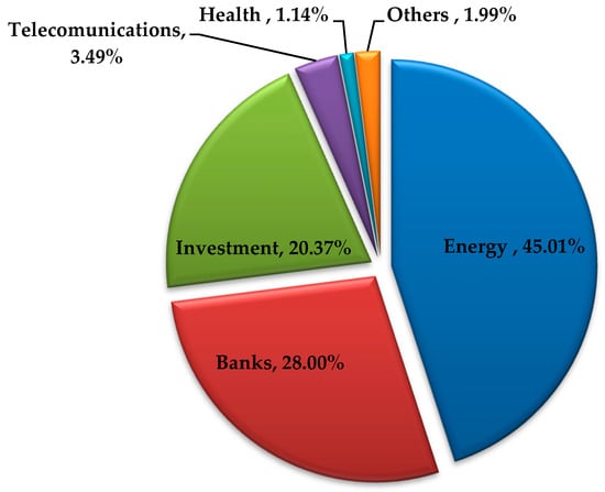
Figure 1. BET index sector weights (as of February 2019). Source: Authors’ work based on the Bucharest Stock Exchange data.

3.2. Econometric Methods

In this article, we intend to determine whether the energy market has an influence on the functioning of the Romanian capital market. In order to reach a relevant conclusion, we will apply several econometric models that will allow us to obtain opinion on how the evolution of the energy market affects the evolution of the Romanian capital market. Due to the availability of certain indicators, we will use both annual and monthly data.

In determining our main objective, we will use the Johansen cointegration test, VAR/VECM models, impulse-response functions, autoregressive distributed lag (ARDL), and the Granger causality test.

One of the first steps in econometric analysis is to test for the unit roots of the series. For the purposes of this paper, the augmented Dickey–Fuller (ADF) unit root test will be employed to check the non-stationary assumption. The ADF test involves estimating the equation [20,21,25,36,60,65,69]:

$$\Delta {\mathrm{y}}_{\mathrm{t}}=\mathsf{\alpha }+\mathsf{\beta }\mathrm{t}+\mathrm{q}{\mathrm{y}}_{\mathrm{t}}+{{\displaystyle \sum }}_{\mathrm{j}=1}^{\mathrm{k}}{\mathsf{\gamma }}_{\mathrm{j}}\Delta {\mathrm{y}}_{\mathrm{t}-\mathrm{j}}+{\mathsf{\epsilon }}_{\mathrm{t}},\mathrm{t}=1,\dots ,\mathrm{T}$$

(1)

where t is a time trend, T = length sample (131), and k measures the length of the lag in the dependent variable. The null hypothesis supposes that the variable has a unit root, and the alternative is that the variable was generated by a stationary process.

Further, we will employ the cointegration test developed by Johansen [70]. We will consider a VAR of the order, p [13,14,15,22,25,35,40,44,45,65]:

$${\mathrm{y}}_{\mathrm{t}}={\mathrm{A}}_1{\mathrm{y}}_{\mathrm{t}-1}+\dots +{\mathrm{A}}_{\mathrm{p}}{\mathrm{y}}_{\mathrm{t}-\mathrm{p}}+{\mathrm{Bx}}_{\mathrm{t}}+{\mathsf{ϵ}}_{\mathrm{t}}$$

(2)

where ${\mathrm{y}}_{\mathrm{t}}$ is a vector of non-stationary variables, ${\mathrm{x}}_{\mathrm{t}}$ is a vector of deterministic variables, and ${\mathsf{ϵ}}_{\mathrm{t}}$ is a vector of innovations. The above equation can be rewritten as:

$$\Delta {\mathrm{y}}_{\mathrm{t}}={\mathrm{Cy}}_{\mathrm{t}-1}+{{\displaystyle \sum }}_{\mathrm{i}=1}^{\mathrm{p}-1}{\mathrm{D}}_{\mathrm{i}}\Delta {\mathrm{y}}_{\mathrm{t}-\mathrm{i}}+{\mathrm{Bx}}_{\mathrm{t}}+{\mathsf{ϵ}}_{\mathrm{t}},$$

(3)

where $\mathrm{C}={{\displaystyle \sum }}_{\mathrm{i}=1}^{\mathrm{p}}{\mathrm{A}}_{\mathrm{i}}-\mathrm{I}$ and ${\mathrm{D}}_{\mathrm{i}}=-{{\displaystyle \sum }}_{\mathrm{j}=\mathrm{i}+1}^{\mathrm{p}}{\mathrm{A}}_{\mathrm{ij}}$.

Many researchers [1,10,26,30,36,39,40,59,60,64] use the autoregressive-distributed lag model (ARDL) and the bounds testing methodology because these models can be used with a mixture of I(0) and I(1) data. In our study, we have both stationary and non-stationary variables so this approach will help in our research.

An ARDL (p,${\mathrm{q}}_1$,…$,{\mathrm{q}}_{\mathrm{k}})$ is a least squares regression containing lags of the dependent (p) and explanatory variables (${\mathrm{q}}_1$,…,${\mathrm{q}}_{\mathrm{k}})$ [71].

An ARDL (p,q) model may be written as:

$${\mathrm{Y}}_{\mathrm{t}}=\mathsf{\mu }+{\mathsf{\beta }}_0{\mathrm{X}}_{\mathrm{t}}+{\mathsf{\beta }}_1{\mathrm{X}}_{\mathrm{t}-1}+\dots +{\mathsf{\beta }}_{\mathrm{q}0}{\mathrm{X}}_{\mathrm{t}-\mathrm{q}}+{\mathsf{\delta }}_1{\mathrm{Y}}_{\mathrm{t}-1}+\dots +{\mathsf{\delta }}_{\mathrm{p}}{\mathrm{Y}}_{\mathrm{t}-\mathrm{p}}+{\mathrm{u}}_{\mathrm{t}}$$

(4)

According to the literature, to analyze the causality between two variables, the Granger causality test can be used [29,60,65,72]. The null hypothesis is that x does not Granger-cause y in the first regression and that y does not Granger-cause x in the second regression. We have the following bivariate regressions:

$${\mathrm{y}}_{\mathrm{t}}={\mathsf{\alpha }}_0+{\mathsf{\alpha }}_1{\mathrm{y}}_{\mathrm{t}-1}+\dots +{\mathsf{\alpha }}_{\mathrm{p}}{\mathrm{y}}_{\mathrm{t}-\mathrm{p}}+{\mathsf{\beta }}_1{\mathrm{x}}_{\mathrm{t}-1}+\dots +{\mathsf{\beta }}_{\mathrm{p}}{\mathrm{x}}_{-\mathrm{p}}+{\mathsf{ϵ}}_{\mathrm{t}}$$

(5)

$${\mathrm{x}}_{\mathrm{t}}={\mathsf{\alpha }}_0+{\mathsf{\alpha }}_1{\mathrm{x}}_{\mathrm{t}-1}+\dots +{\mathsf{\alpha }}_{\mathrm{p}}{\mathrm{x}}_{\mathrm{t}-\mathrm{p}}+{\mathsf{\beta }}_1{\mathrm{y}}_{\mathrm{t}-1}+\dots +{\mathsf{\beta }}_{\mathrm{p}}{\mathrm{y}}_{-\mathrm{p}}+{\mathrm{u}}_{\mathrm{t}}$$

(6)

4. Empirical Findings and Discussion

4.1. Summary Statistics and Correlation Analysis

Table 3 displays the descriptive statistics of the variables (logarithmic data). The skewness indicator is used to analyze the distribution of a series of data to indicate the deviation in relation to a symmetric distribution around the average. Most of the variables have negative skewed data, in which the “tail” of the distribution points to the left. The Kurtosis indicator is used in the analysis of the distribution of a series of data to indicate the degree of flattening or sharpening. In our case, the variables have a Kurtosis value greater than 3 for most of the variables, thus presenting a leptokurtic distribution, with more values centered on the mean and heavy tails, which means high probabilities for extreme values.

Table 3. Descriptive statistics of the variables.

Variables	Obs.	Mean	Std. Dev.	Skewness	Kurtosis	Jarque-Bera	Jarque-Bera Probability
LNBET	112	8.669	0.264	–1.445	6.275	88.996	0.000
LNBIODIESELS	112	2.329	0.704	–1.158	4.001	29.722	0.000
LNCOKEOVENCOKE	112	4.148	0.509	–2.739	12.950	602.082	0.000
LNGASDIESELOIL	112	5.953	0.185	–0.883	3.643	16.463	0.000
LNHARDCOAL	112	4.380	0.518	0.833	4.852	28.954	0.000
LNKEROSENE	112	2.305	0.449	–1.078	4.460	31.622	0.000
LNLIGNITE_BROWNCOAL	112	7.757	0.228	–0.444	2.779	3.912	0.141
LNLPG	112	3.915	0.158	–0.451	3.098	3.842	0.146
LNMOTORGASOLINE	112	4.748	0.208	–0.341	3.110	2.233	0.327
LNNAPHTHA	112	2.867	0.510	–1.193	6.116	71.863	0.000
LNOIL	112	–2.000	0.519	1.207	4.264	34.632	0.000
LNPETROLEUMCOKE	112	3.687	0.475	–0.726	3.887	13.524	0.001
LNPTR	112	–0.997	0.272	0.538	2.914	5.433	0.066
LNREFINERYGAS	112	1.932	0.460	0.308	3.390	2.479	0.290
LNROADDIESEL	112	5.932	0.188	–0.899	3.693	17.312	0.000
LNSNP	112	–1.000	0.274	–0.871	3.966	18.518	0.000
LNWTI	112	4.290	0.348	–0.423	1.913	8.859	0.012
LNCO2	20	11.830	0.120	–0.188	1.877	1.170	0.56

Source: Authors’ calculations.

To test the normality of the variable distribution, we used the Jarque-Bera test in EViews. Table 3 shows the results of the Jarque-Bera test, which indicate that the variables’ distribution is not distributed normally—the probability associated with it being 0—with the exception for the data series, LNLIGNITEBROWNCOAL, LNLPG, LNMOTORGASOLINE, LNREFINARYGAS, and LNCO2, which are normally distributed. In addition, the correlations between the energy market and capital market variables are provided in Table 4.

Table 4. Correlation matrix.

Variables		1	2	3	4		5	6	7	8
1	LNBET	1
2	LNBIODIESELS	0.019837	1
3	LNCOKEOVENCOKE	0.302639 **	0.056402	1
4	LNGASDIESELOIL	0.294173 **	0.506691 ***	0.152773	1
5	LNHARDCOAL	–0,205658 *	–0.186641 *	0.116550	–0.198480 *		1
6	LNKEROSENE	–0.224338 *	0.379759 ***	0.301373 **	0.206797 *		0.267411 **	1
7	LNLIGNITE_BROWNCOAL	–0.381451 ***	–0.060636	0.163637	–0.053999		0.403372 ***	0.449909 ***	1
8	LNLPG	0.486944 ***	0.262153 **	0.067080	0.685985 ***		–0.076180	0.116272	–0.137539	1
9	LNMOTORGASOLINE	–0.153176	0.421622 ***	0.162057	0.451096 ***		0.017844	0.367806 ***	0.176028	0.312964 ***
10	LNNAPHTHA	–0.264576 **	0.146914	–0.097473	–0.109589		0.342754 ***	0.223665 *	0.168755	–0.016386
11	LNOIL	–0.168808	0.051095	0.181445	–0.214490 *		0.617855 ***	0.418831 ***	0.543073 ***	–0.204072 *
12	LNPETROLEUMCOKE	0.237965 *	0.125421	–0.058735	0.211975 *		0.142200	0.008375	0.050026	0.404952 ***
13	LNPTR	0.373404 ***	–0.177492	0.088181	–0.168382		0.205093 *	–0.130723	–0.059304	0.006590
14	LNREFINERYGAS	–0.466324 ***	–0.074417	0.102623	–0.376549 ***		0.283673 ***	0.311054 ***	0.410634 ***	–0.418005 ***
15	LNROADDIESEL	0.295797 **	0.521459 ***	0.159496	0.997894 ***		–0.196566 *	0.220585 *	–0.043773	0.684611 ***
16	LNSNP	0.453917 ***	–0.112876	0.326782 ***	–0.026363		0.020845	–0.149667	0.017320	–0.069653
17	LNWTI	–0.154106	–0.070255	0.179022	–0.210518 *		0.264572 **	0.136983	0.357137 ***	–0.370116 ***
Variables		9	10	11	12	13	14	15	16	17
9	LNMOTORGASOLINE	1
10	LNNAPHTHA	0.247586 **	1
11	LNOIL	0.135107	0.410597 ***	1
12	LNPETROLEUMCOKE	0.032217	0.004021	–0.081141	1
13	LNPTR	–0.017205	0.262863 **	0.397021 ***	0.010538	1
14	LNREFINERYGAS	0.062327	0.240188 *	0.493485 ***	–0.352170 ***	–0.057429	1
15	LNROADDIESEL	0.451411 ***	–0.105440	–0.205540 *	0.210668 *	–0.186680 *	–0.370143 ***	1
16	LNSNP	–0.153259	–0.171836	0.138726	–0.039764	0.568214 ***	–0.013468	–0.039758	1
17	LNWTI	–0.013816	0.088698	0.517778 ***	–0.223729 *	0.451084 ***	0.434059 ***	–0.224446 *	0.687447 ***	1

Source: Authors’ calculations. Notes: * p < 0.05, ** p < 0.01, *** p < 0.001.

The correlation coefficient measures the strength of the linear relationship between two variables and takes values between [−1,1]. The correlations close to zero represent no linear association between the variables, whereas correlations close to −1 or +1 indicate a strong linear relationship. We see some positive correlations that are significantly different from zero between energy market variables and capital market variables (strong relationship between WTI and listed company oil terminal, gas, diesel oil, and biodiesels, road diesel, and listed company oil terminal, liquefied petroleum, gas, and gas diesel oil, etc.)

4.2. Causality Investigation

Some have claimed that non-stationary series produce spurious results, which means non-sense results. Therefore, in order to avoid spurious results, the variables must be stationary. In our study, the stationary of the data is checked through ADF test, as reported in Table 5, which is commonly used in research studies.

Table 5. The outcomes of the augmented Dickey-Fuller test.

Variables	Level	First Difference
LNBET	–1.68	–7.48 ***
LNBIODIESELS	–0.24	–11.97 ***
LNCOKEOVENCOKE	–6.78 ***	–11.026 ***
LNGASDIESELOIL	0.35	–12.56 ***
LNHARDCOAL	–6.36 ***	–13.71 ***
LNKEROSENE	–2.53	–7.82 ***
LNLIGNITEBROWNCOAL	–1.29	–3.94 ***
LNLPG	–0.80	–8.09 ***
LNMOTORGASOLINE	–1.41	–8.54 ***
LNNAPHTHA	–2.78 *	–5.88 ***
LNOIL	–3.05 **	–6.50 ***
LNPETROLEUMCOKE	–4.85 ***	–6.42 ***
LNPTR	–3.32 **	–11.45 ***
LNREFINERYGAS	–1.50	–9.23 ***
LNROADDIESEL	0.38	–6.01 ***
LNSNP	–2.16	–5.48 ***
LNWTI	–2.31	–7.81 ***
LNCO2	1.33	–3.49 ***

Source: Authors’ calculations. Notes: *, **, and *** indicates the rejection of the null hypothesis: series Has a unit root at the 10%, 5%, and 1% level of significance.

According to the results found in Table 5, the probability associated with the ADF test is below the 1%/5% relevance level for the variables of LNCOKEOVENCOKE, LNHARDCOAL, LNOIL, LNPETROLEUMCOKE, and LNPTR, so we can reject the null hypothesis and conclude that the series are stationary, and that the mean and variance of the series is constant over time.

Choosing the number of lags can be done by studying the information criteria exposed in Table 6. Information criteria are the initial measures that can be adopted when selecting the appropriate ‘lag length’ in a time series.

Table 6. Choosing the number of lags.

Variables	No. of Lags					Selected Lag
	LR	FPE	AIC	SC	HQ
LNBIODIESELS	4	4	4	2	4	4
LNGASDIESELOIL	3	4	6	1	2	4
LNKEROSENE	7	7	7	2	2	7
LNLIGNITEBROWNCOAL	4	2	2	2	2	2
LNLPG	4	5	5	2	4	5
LNMOTORGASOLINE	6	6	6	1	2	6
LNNAPHTHA	4	4	4	1	2	4
LNREFINERYGAS	4	4	4	2	2	4
LNROADDIESEL	4	4	4	1	2	4
LNSNP	4	4	4	2	4	4
LNWTI	4	4	4	2	3	4
LNCOKEOVENCOKE	6	2	2	2	2	2
LNHARDCOAL	5	5	5	1	4	5
LNPETROLEUMCOKE	4	4	4	1	4	4
LNOIL	5	5	5	2	5	5
LNPTR	7	7	7	1	2	7
LNCO2	1	1	1	1	1	1

Source: Authors’ calculations.

A precondition for applying the Johansen cointegration test is that the variables must be non-stationary and integrated by the same order, conditions that are met. The outcomes of the Johansen co-integration test are shown in Table 7, with two results: Trace test and maximum eigenvalue. For the trace test results, the first hypothesis is that there is no cointegration and the second one that at most (–1), there is a cointegration relationship. Additionally, for the maximum eigenvalue, the way the data is interpreted is the same as with the trace test.

Table 7. The results of the Johansen test.

Variables	Unrestricted Cointegration Rank Test	Trace (Prob.)	Maximum Eigenvalue (Prob.)
LNBET-LNBIODIESELS	None	0.0000	0.0000
	At most 1	0.0055	0.0055
LNBET-LNGASDIESELOIL	None	0.0000	0.0001
	At most 1	0.0201	0.0201
LNBET-LNKEROSENE	None	0.1686	0.2949
	At most 1	0.0903	0.0903
LNBET-LNLIGNITEBROWNCOAL	None	0.0009	0.0013
	At most 1	0.1087	0.1087
LNBET-LNPG	None	0.0002	0.0005
	At most 1	0.0543	0.0543
LNBET-LNMOTORGASOLINE	None	0.0002	0.0007
	At most 1	0.0346	0.0346
LNBET-LNNAPHTHA	None	0.0017	0.0107
	At most 1	0.0137	0.0137
LNBET-LNREFINERYGAS	None	0.0460	0.0494
	At most 1	0.2301	0.2301
LNROADDIESEL	None	0.0000	0.0001
	At most 1	0.0192	0.0192
LNBET-LNSNP	None	0.0362	0.0309
	At most 1	0.3583	0.3583
LNBET-LNWTI	None	0.0160	0.0117
	At most 1	0.4496	0.4496
LNBET-LNCO2	At most 1	0.2161	0.2161
	None	0.3519	0.4189

Source: Authors’ calculations.

According to the results from Table 7 of the variables that represent the energy market only, LNKEROSENE and LNCO2 do not have a long-term relationship with the Romanian capital market. From the BSE traded shares, all of them have a long-term relationship with the BET index.

Using VECM for those variables that have a cointegration relationship and VAR for non-cointegrated variables, we can see the causality between the energy market and the capital market. Applying these econometric models also allows us to verify the existence of the short-term relationship between these two main markets.

C(1) is the error correction term or the speed of adjustment towards long-term equilibrium. According to the results reported in Table 8, from estimating the equations, the coefficient, C(1), is negative and statistically significant only for LNGASDIESELOIL, LNLIGNITEBROWNCOAL, LNNAPHTHA, LNREFINERYGAS, LNROADDIESE, L and LNSNP, which means there is long-lasting causality on the part of the variables that represent the energy domain to the Romanian capital market. Moreover, the West Texas Intermediate (WTI) oil price, a reference in the US market, has a long-term influence on our local capital market. The long-term causality of the energy market on the capital market is confirmed, but not all energy market indicators have a long-term influence on the stock market.

Table 8. The outcomes of the C(1) coefficient and Wald test.

Variables	C(1) (Value, p-Value)	Wald Test (F-Statistic)
LNBIODIESELS	0.000391, 0.8750	0.3151
LNGASDIESELOIL	–0.059197, 0.0128	0.0041
LNKEROSENE	1.422164, 0.0000	0.8871
LNLIGNITEBROWNCOAL	–0.046490, 0.0458	0.0458
LNLPG	–0.042521, 0.1106	0.0337
LNMOTORGASOLINE	–0.002714, 0.8584	0.2554
LNNAPHTHA	–0.087209, 0.0016	0.0686
LNREFINERYGAS	–0.096225, 0.0009	0.0457
LNROADDIESEL	–0.056744, 0.0156	0.0048
LNSNP	–0.030277, 0.0002	0.3064
LNWTI	–0.071507, 0.0002	0.0489
LNCO2	0.844634, 0.0000	0.3829

Source: Authors’ calculations.

The short-term causality can be verified by applying the Wald test. The probability is above 5%, which allows us to accept the null hypothesis, and we can confirm the absence of short-term causality from the energy market to the stock market. In the case of the variables, LNGASDIESELOIL, LNLIGNITEBROWNCOAL, LNLPG, LNREFINERYGAS, LNROADDIESEL, and LNWTI, the presence of a short-term causality from the energy market to the capital market is confirmed, according to the Wald test.

The impulse response function and variance decomposition are shown in Figure 2 and permit us to check the behavior of one variable in response to innovations of another variable in the future. However, the impulse response function explains how much the LNBET variable responds to other variables’ shocks. The horizontal axis (X) of the chart represents the number of periods and the vertical axis (Y) shows the amount of the variable expected to change following a unit impulse.

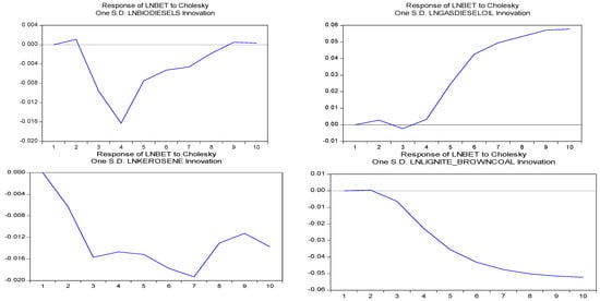
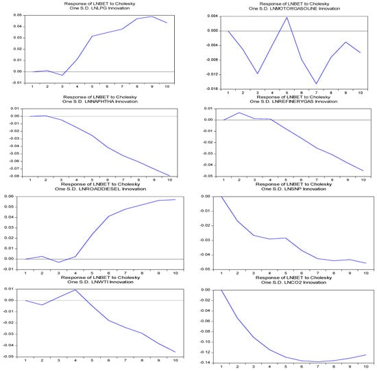
Figure 2. Impulse-response functions. Source: Authors’ work.

By applying the impulse-response functions, we can identify how the impact of the market energy, represented by various indicators, looks like on the capital market. As seen from the graphs above, there are a group of variables that have had a negative impact since the first period on the BET index. Although it initially shows a slight decrease in the first range, they gradually increase along the way (LNGASDIESELOIL, LNLPG, and LNROADDIESEL).

The variance decomposition exhibited in Table 9 explains how much the energy market and capital market variables contribute to the explanation of the BET variable.

Table 9. Variance decomposition.

Period	LNBIODIESELS	LNGASDIESELOIL	LNKEROSENE	LNLIGNITEBROWNCOAL	LNLPG	LNMOTORGASOLINE
1	0.000000	0.000000	0.000000	0.000000	0.000000	0.000000
2	0.008435	0.060778	0.242017	0.001701	0.008453	0.176719
3	0.378916	0.065720	1.021310	0.183346	0.050265	0.643361
4	1.003426	0.082615	1.218346	1.877389	0.429810	0.473112
5	0.822535	1.457270	1.244091	4.879756	2.467062	0.356942
6	0.663140	4.169189	1.380386	8.146468	3.887900	0.367541
7	0.556186	6.639736	1.559117	11.15242	5.180235	0.559518
8	0.462366	8.665825	1.498315	13.75194	6.978590	0.533991
9	0.390719	10.40187	1.406995	15.92905	8.431184	0.473832
10	0.337200	11.72497	1.389392	17.72764	9.190025	0.450882
Period	LNNAPHTHA	LNREFINERYGAS	LNROADDIESEL	LNSNP	LNWTI	LNCO2
1	0.000000	0.000000	0.000000	0.000000	0.000000	0.000000
2	0.003096	0.324156	0.051732	2.279641	0.138500	1.827051
3	0.102637	0.223559	0.077700	5.301670	0.141625	1.412508
4	0.811653	0.167780	0.072658	7.241695	0.494297	2.106627
5	2.192161	0.283645	1.334785	7.893597	0.447065	4.922611
6	4.929504	0.780374	3.860445	9.764183	1.207580	9.284095
7	8.339854	1.819206	6.194822	12.32793	2.440293	14.17315
8	11.93322	3.190016	8.167273	14.85113	4.089324	18.82026
9	15.84959	5.076928	9.892050	17.09041	6.743225	22.89836
10	20.05696	7.492947	11.21554	19.60460	10.24462	26.36051

Source: Authors’ calculations.

In the first period, the variance decomposition of BET is exclusively generated by its own innovations (for all variables). The contributions of LNGASDIESELOIL, LNLIGNITEBROWNCOAL, LNLPG, LNNAPHTHA, LNREFINERYGAS, LNROADDIESEL, LNSNP, LNWTI, and LNCO2 in explaining the LNBET forecast error variance increased during the 10th forecast period, but there are no significant changes in the contribution of LNBIODIESELS, LNKEROSENE, and LNMOTORGASOLINE.

From the results obtained after the variance decomposition, it can be noticed that the LNCO2 variable records the most significant contribution in the LNBET explanation with a value of 26.36% in the 10th forecasting period.

According to the specialized literature, to analyze the causality between two variables, the Granger causality test can be used. In order to be able to apply the Granger causality test, the data series must be stationary and the mean must be 0. After their transformation, we obtained the following results, which are shown in Table 10.

Table 10. The results of the Granger causality test.

Null Hypothesis	F-Statistic	Prob.
DLNBIODIESELS does not Granger Cause DLNBET	1.32353	0.2653
DLNBET does not Granger Cause DLNBIODIESELS	0.09749	0.9831
DLNGASDIESELOIL does not Granger Cause DLNBET	2.35200	0.0580
DLNBET does not Granger Cause DLNGASDIESELOIL	1.22840	0.3026
DLNKEROSENE does not Granger Cause DLNBET	0.40646	0.8963
DLNBET does not Granger Cause DLNKEROSENE	1.49439	0.1780
DLNLIGNITEBROWNCOAL does not Granger Cause DLNBET	0.64722	0.5253
DLNBET does not Granger Cause DLNLIGNITEBROWNCOAL	0.44476	0.6420
DLNLPG does not Granger Cause DLNBET	2.17514	0.0617
DLNBET does not Granger Cause DLNLPG	1.14795	0.3394
DLNMOTORGASOLINE does not Granger Cause DLNBET	1.41031	0.2169
DLNBET does not Granger Cause DLNMOTORGASOLINE	0.84028	0.5414
DLNNAPHTHA does not Granger Cause DLNBET	0.20804	0.9334
DLNBET does not Granger Cause DLNNAPHTHA	0.19171	0.9422
DLNREFINERYGAS does not Granger Cause DLNBET	1.14505	0.3392
DLNBET does not Granger Cause DLNREFINERYGAS	0.42684	0.7890
DLNROADDIESEL does not Granger Cause DLNBET	2.34823	0.0584
DLNBET does not Granger Cause DLNROADDIESEL	1.15396	0.3348
DLNSNP does not Granger Cause DLNBET	1.87925	0.1186
DLNBET does not Granger Cause DLNSNP	4.16508	0.0034
DLNWTI does not Granger Cause DLNBET	2.45496	0.0496
DLNBET does not Granger Cause DLNWTI	1.92364	0.1110
LNCOKEOVENCOKE does not Granger Cause DLNBET	0.07349	0.9292
DLNBET does not Granger Cause LNCOKEOVENCOKE	8.22567	0.0005
LNHARDCOAL does not Granger Cause DLNBET	2.81054	0.0197
DLNBET does not Granger Cause LNHARDCOAL	4.42659	0.0010
LNPETROLEUMCOKE does not Granger Cause DLNBET	1.20128	0.3143
DLNBET does not Granger Cause LNPETROLEUMCOKE	1.69044	0.1572
LNOIL does not Granger Cause DLNBET	2.43211	0.0391
DLNBET does not Granger Cause LNOIL	2.76777	0.0213
LNPTR does not Granger Cause DLNBET	3.78945	0.0010
DLNBET does not Granger Cause LNPTR	1.64743	0.1299
DLNCO2 does not Granger Cause DLNBET	0.09129	0.7667
DLNBET does not Granger Cause DLNCO2	15.3506	0.0014

Source: Authors’ calculations.

Of all the indicators we have chosen as being representative of the Romanian energy market, only hard coal has a bidirectional relationship to the Romanian capital market. Instead, according to the Granger test, the BET index appears to be in a one-way causal relationship with some of them, such as C0₂, OIL, and SNP. It is also evident that the energy market from America, represented by the WTI, influences the Romanian capital market through a unidirectional causal relationship from the US energy market to the local stock exchange.

Many researchers use the autoregressive-distributed lag model (ARDL) and the bounds testing methodology, due to the number of features of these two offer over the conventional cointegration testing. These models can be used with a mixture of I(0) and I(1) data, and involves just a single equation to be set up, making it simple to implement and interpret and different variables can be assigned different lag-lengths as they enter the model. So, these models can be used to test for cointegration, and estimate long-term and short-term dynamics, even when the variables in question may include a mixture of stationary and non-stationary time-series.

Considering the results of the ADF test from Table 5, the analyzed variables include a mixture of stationary and non-stationary time-series.

Furthermore, in Figure 3, the optimal lag lengths criteria are included and we applied Akaike information criteria (AIC) to choose optimal lags for the variables included in the ARDL model. The criteria graph indicates the right lags for the ARDL model. The horizontal axis (X) of the chart represents the ARDL models estimated and the vertical axis (Y) shows the AIC value of the models. The lowest value is preferred.

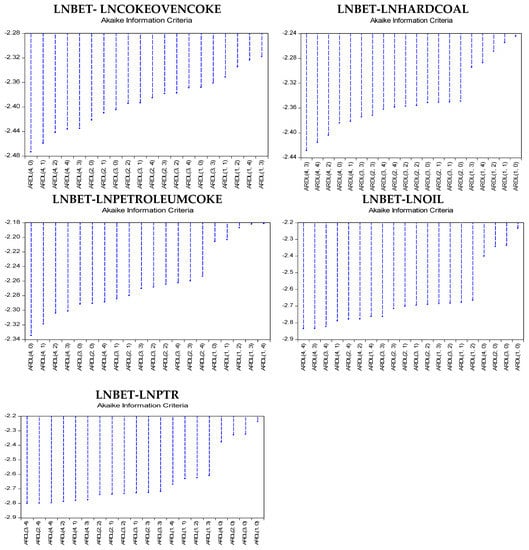
Figure 3. Optimal lags. Source: Authors’ work.

The results reported in Table 11 are out of EViews 9 and the software automatically selected the number of lags for the five analyzed variables.

Table 11. The results of the ARDL bounds test.

Null Hypothesis: No Long-Run Relationships Exist	F-Statistic
LNCOKEOVENCOKE	2.08557
LNHARDCOAL	7.779161
LNOIL	10.35561
LNPETROLEUMCOKE	2.160678
LNPTR	1.319994
Critical Value Bounds
Significance	I0 Bound	I1 Bound
10%	4.04	4.78
5%	4.94	5.73
2.50%	5.77	6.68
1%	6.84	7.84

Source: Authors’ calculations.

The ARDL bound test for cointegration is based on the F-statistic. Two critical values are given by Pesaran et al. [73] for the cointegration test. The lower critical bound assumes all the variables are I(0), meaning that there is no cointegration relationship between the examined variables. The upper bound assumes that all the variables are I(1), meaning that there is cointegration among the variables. When the computed F-statistic is greater than the upper bound critical value, then the H0 is rejected, meaning that the variables in the model are cointegrated.

Only LNHARCOAL and LNOIL have an F-statistics value greater than the upper bound, which suggests that the a long-term relationship exists between them and the BET index.

Table 12 shows out the results of the long-term relationship between variables. Hard coal and the share stock oil coefficients are significant at the 5% level of significance. For instance, the coefficient value of LNHARCOAL (–0.676532) indicates that an increase of one unit in LNHARCOAL leads to over a –0.676532 units decrease in LNBET in the long-term.

Table 12. ARDL cointegrating and long-term form, long-term coefficients.

Variables	Coefficient	Std. Error	t-Statistic	Prob.	CointEq(–1)
LNHARDCOAL	–0.676532	0.267828	–2.525995	0.0129	–0.078588 (0.001)
LNOIL	–0.524756	0.185585	–2.827569	0.0055	–0.07528 (0.0001)

Source: Authors’ calculations.

The coefficient of the error correction term (CointEq(–1)) is significant at the 5% level of significance. The negative and significant error correction term, which indicates the speed of conversion, show that in the next month, the dependent variable (LNBET) will reach equilibrium with a speed of 7.85% (LNHARCOAL) and 7.52% (LNOIL).

5. Conclusions and Policy Implications

The energy sector can contribute to economic growth and job creation in some countries, even if the share of energy in the GDP is rather modest. The main objective of this research was to determine whether there is any influence from the Romanian energy market on the Romanian capital market. In this study, we undertook two large series of indicators: Those representing the energy market (supply and transformation of oil: Biodiesels, gas diesel oil, kerosene, liquefied petroleum gas, motor gasoline, naphtha, petroleum coke, refinery gas, road diesel; supply and transformation of solid fuels: Coke oven coke, hard coal, lignite brown coal; greenhouse gas emissions: CO₂) and those representing the capital market (stock indices for the Bucharest Stock Exchange, the representative benchmark for oil prices—West Texas Intermediate (WTI), and companies listed on the Bucharest Stock Exchange that carry out activities in the energy industry). The variables chosen to represent the energy market consist of the supply and transformation of oil and greenhouse gas emissions. In addition, the BET index (for Romania), WTI (as a benchmark in oil pricing), and some companies listed on the BSE in the field of energy were used as a proxy for the capital market. Our data sample was monthly (January 2008–November 2018) and annual (1997–2016).

Our results provide empirical evidence regarding the long-term and short-term relationships between energy market indicators and the Romanian stock market. To the best of our knowledge, this is the first investigation to examine the linkage between the energy market and the Romanian stock market. Therefore, we believe we are making an important addition to academic activity and to investors interested in the energy field and beyond.

Taking into account the results obtained after applying the ADF stationarity test, our variables showed a mix of stationarity and non-stationarity. In order to study the cointegration relationships between variables, we used the Johansen cointegration test for those that have the same integration order and the ARDL model for those with a mixed stationarity. The empirical evidence suggests the presence of a long-term relationship between the studied variables, with the exception of kerosene.

The approach of the ARDL model to the analysis of the relationship between variables represents a new method used by the researchers and provides added value to the existing literature by addressing, in our research, the relationship between the energy and capital market using Romania as a case study. We emphasize the importance of the ARDL model, which can be used to test for cointegration, and estimate long-term and short-term dynamics, even when the variables in question may include a mixture of stationary and non-stationary time-series.

Additionally, the empirical findings from the VAR/VECM models showed the presence of a short-term causality from the energy market (gas diesel oil, lignite brown coal, liquefied petroleum gas, refinery gas, road diesel, and WTI) to the stock market. Of all the indicators we selected as being representative of the Romanian energy market, we found empirical evidence that hard coal presented a causal relationship with the BET index. The results provided by the Granger test provide support for the existence of bidirectional causality between hard coal and the BET index.

Our results identify that the American energy market, represented by the WTI, influences the Romanian capital market through a unidirectional causal relationship from the US energy market to the local stock exchange.

Through this research, we believe we provided empirical evidence of the long-term and short-term relationships between energy market indicators and Romanian stock markets. Our findings should be of interest to researchers, regulators, and market participants.

References

- Dutta, A. Oil and energy sector stock markets: An analysis of implied volatility indexes. J. Multinatl. Financ. Manag. 2018, 44, 61–68. [Google Scholar] [CrossRef]
- Kumar, S.; Managi, S.; Matsuda, A. Stock prices of clean energy firms, oil and carbon markets: A vector autoregressive analysis. Energy Econ. 2012, 34, 215–226. [Google Scholar] [CrossRef]
- Zhang, Y.-J.; Wang, J.-L. Do high-frequency stock market data help forecast crude oil prices? Evidence from the midas models. Energy Econ. 2019, 78, 192–201. [Google Scholar]
- Smyth, R.; Narayan, P.K. What do we know about oil prices and stock returns? Int. Rev. Financ. Anal. 2018, 57, 148–156. [Google Scholar] [CrossRef]
- Yu, H.H.; Du, D.L.; Fang, L.B.; Yan, P.P. Risk contribution of crude oil to industry stock returns. Int. Rev. Econ. Financ. 2018, 58, 179–199. [Google Scholar] [CrossRef]
- Thorbecke, W. How oil prices affect east and southeast asian economies: Evidence from financial markets and implications for energy security. Energy Policy 2019, 128, 628–638. [Google Scholar] [CrossRef]
- Hamdi, B.; Aloui, M.; Alqahtani, F.; Tiwari, A. Relationship between the oil price volatility and sectoral stock markets in oil-exporting economies: Evidence from wavelet nonlinear denoised based quantile and granger-causality analysis. Energy Econ. 2019, 80, 536–552. [Google Scholar] [CrossRef]
- Tiwari, A.K.; Jena, S.K.; Mitra, A.; Yoon, S.M. Impact of oil price risk on sectoral equity markets: Implications on portfolio management. Energy Econ. 2018, 72, 120–134. [Google Scholar] [CrossRef]
- Reboredo, J.C. Is there dependence and systemic risk between oil and renewable energy stock prices? Energy Econ. 2015, 48, 32–45. [Google Scholar] [CrossRef]
- Kocaarslan, B.; Soytas, U. Asymmetric pass-through between oil prices and the stock prices of clean energy firms: New evidence from a nonlinear analysis. Energy Rep. 2019, 5, 117–125. [Google Scholar] [CrossRef]
- Cong, R.G.; Wei, Y.M. Potential impact of (cet) carbon emissions trading on china’s power sector: A perspective from different allowance allocation options. Energy 2010, 35, 3921–3931. [Google Scholar] [CrossRef]
- Ferrer, R.; Shahzad, S.J.H.; Lopez, R.; Jareno, F. Time and frequency dynamics of connectedness between renewable energy stocks and crude oil prices. Energy Econ. 2018, 76, 1–20. [Google Scholar] [CrossRef]
- Managi, S.; Okimoto, T. Does the price of oil interact with clean energy prices in the stock market? Jpn. World Econ. 2013, 27, 1–9. [Google Scholar] [CrossRef]
- Luo, X.G.; Qin, S.H. Oil price uncertainty and chinese stock returns: New evidence from the oil volatility index. Financ. Res. Lett. 2017, 20, 29–34. [Google Scholar] [CrossRef]
- Sun, C.W.; Ding, D.; Fang, X.M.; Zhang, H.M.; Li, J.L. How do fossil energy prices affect the stock prices of new energy companies? Evidence from divisia energy price index in china’s market. Energy 2019, 169, 637–645. [Google Scholar] [CrossRef]
- Salisu, A.A.; Raheem, I.D.; Ndako, U.B. A sectoral analysis of asymmetric nexus between oil price and stock returns. Int. Rev. Econ. Financ. 2019, 61, 241–259. [Google Scholar] [CrossRef]
- Angelidis, T.; Degiannakis, S.; Filis, G. Us stock market regimes and oil price shocks. Glob. Financ. J. 2015, 28, 132–146. [Google Scholar] [CrossRef]
- Bagirov, M.; Mateus, C. Oil prices, stock markets and firm performance: Evidence from europe. Int. Rev. Econ. Financ. 2019, 61, 270–288. [Google Scholar] [CrossRef]
- Narayan, P.K.; Phan, D.H.B.; Sharma, S.S. Does islamic stock sensitivity to oil prices have economic significance? Pac. Basin Financ. J. 2019, 53, 497–512. [Google Scholar] [CrossRef]
- Fowowe, B. Jump dynamics in the relationship between oil prices and the stock market: Evidence from nigeria. Energy 2013, 56, 31–38. [Google Scholar] [CrossRef]
- Cunado, J.; de Gracia, F.P. Oil price shocks and stock market returns: Evidence for some european countries. Energy Econ. 2014, 42, 365–377. [Google Scholar] [CrossRef]
- Bastianin, A.; Conti, F.; Manera, M. The impacts of oil price shocks on stock market volatility: Evidence from the g7 countries. Energy Policy 2016, 98, 160–169. [Google Scholar] [CrossRef]
- Gourène, G.A.Z.; Mendy, P. Oil prices and african stock markets co-movement: A time and frequency analysis. J. Afr. Trade 2018, 5, 55–67. [Google Scholar]
- Batten, J.A.; Kinateder, H.; Szilagyi, P.G.; Wagner, N.F. Time-varying energy and stock market integration in asia. Energy Econ. 2019, 80, 777–792. [Google Scholar] [CrossRef]
- Lin, C.-C.; Fang, C.-R.; Cheng, H.-P. Relationships between oil price shocks and stock market: An empirical analysis from greater china. China Econ. J. 2010, 3, 241–254. [Google Scholar] [CrossRef]
- Al-hajj, E.; Al-Mulali, U.; Solarin, S.A. Oil price shocks and stock returns nexus for malaysia: Fresh evidence from nonlinear ardl test. Energy Rep. 2018, 4, 624–637. [Google Scholar] [CrossRef]
- Xiao, J.; Hu, C.; Ouyang, G.; Wen, F. Impacts of oil implied volatility shocks on stock implied volatility in china: Empirical evidence from a quantile regression approach. Energy Econ. 2019, 80, 297–309. [Google Scholar] [CrossRef]
- Xiao, J.H.; Zhou, M.; Wen, F.M.; Wen, F.H. Asymmetric impacts of oil price uncertainty on chinese stock returns under different market conditions: Evidence from oil volatility index. Energy Econ. 2018, 74, 777–786. [Google Scholar] [CrossRef]
- Acaravci, A.; Ozturk, I.; Kandir, S.Y. Natural gas prices and stock prices: Evidence from eu-15 countries. Econ. Model. 2012, 29, 1646–1654. [Google Scholar] [CrossRef]
- Benkraiem, R.; Lahiani, A.; Miloudi, A.; Shahbaz, M. New insights into the us stock market reactions to energy price shocks. J. Int. Financ. Mark. Inst. Money 2018, 56, 169–187. [Google Scholar] [CrossRef]
- Kang, W.S.; Ratti, R.A.; Vespignani, J. The impact of oil price shocks on the us stock market: A note on the roles of us and non-us oil production. Econ. Lett. 2016, 145, 176–181. [Google Scholar] [CrossRef]
- Sim, N.; Zhou, H.T. Oil prices, us stock return, and the dependence between their quantiles. J. Bank. Financ. 2015, 55, 1–8. [Google Scholar] [CrossRef]
- Ahmed, W.M.A. On the dynamic interactions between energy and stock markets under structural shifts: Evidence from egypt. Res. Int. Bus. Financ. 2017, 42, 61–74. [Google Scholar] [CrossRef]
- Ahmed, W.M.A. On the interdependence of natural gas and stock markets under structural breaks. Q. Rev. Econ. Financ. 2018, 67, 149–161. [Google Scholar] [CrossRef]
- Mensi, W. Global financial crisis and co-movements between oil prices and sector stock markets in saudi arabia: A var based wavelet. Borsa Istanb. Rev. 2019, 19, 24–38. [Google Scholar] [CrossRef]
- Bouri, E.; Jain, A.; Biswal, P.C.; Roubaud, D. Cointegration and nonlinear causality amongst gold, oil, and the indian stock market: Evidence from implied volatility indices. Resour. Policy 2017, 52, 201–206. [Google Scholar] [CrossRef]
- Bouri, E. Return and volatility linkages between oil prices and the lebanese stock market in crisis periods. Energy 2015, 89, 365–371. [Google Scholar] [CrossRef]
- Delgado, N.A.B.; Delgado, E.B.; Saucedo, E. The relationship between oil prices, the stock market and the exchange rate: Evidence from mexico. N. Am. J. Econ. Financ. 2018, 45, 266–275. [Google Scholar] [CrossRef]
- Singhal, S.; Choudhary, S.; Biswal, P.C. Return and volatility linkages among international crude oil price, gold price, exchange rate and stock markets: Evidence from mexico. Resour. Policy 2019, 60, 255–261. [Google Scholar] [CrossRef]
- Ersoy, E.; Ünlü, U. Energy consumption and stock market relationship: Evidence from turkey. Int. J. Energy Econ. Policy 2013, 3, 34–40. [Google Scholar]
- Tursoy, T.; Faisal, F. The impact of gold and crude oil prices on stock market in turkey: Empirical evidences from ardl bounds test and combined cointegration. Resour. Policy 2018, 55, 49–54. [Google Scholar] [CrossRef]
- El hédi, E.M.; Julien, F. On the short-term influence of oil price changes on stock markets in gcc countries: Linear and nonlinear analyses. Econ. Bull. 2009, 29, 795–804. [Google Scholar]
- Oberndorfer, U. Energy prices, volatility, and the stock market: Evidence from the eurozone. Energy Policy 2009, 37, 5787–5795. [Google Scholar] [CrossRef]
- Basher, S.A.; Haug, A.A.; Sadorsky, P. Oil prices, exchange rates and emerging stock markets. Energy Econ. 2012, 34, 227–240. [Google Scholar] [CrossRef]
- Masih, R.; Peters, S.; De Mello, L. Oil price volatility and stock price fluctuations in an emerging market: Evidence from south korea. Energy Econ. 2011, 33, 975–986. [Google Scholar] [CrossRef]
- Basta, M.; Molnar, P. Oil market volatility and stock market volatility. Financ. Res. Lett. 2018, 26, 204–214. [Google Scholar] [CrossRef]
- Wen, X.Q.; Wei, Y.; Huang, D.S. Measuring contagion between energy market and stock market during financial crisis: A copula approach. Energy Econ. 2012, 34, 1435–1446. [Google Scholar] [CrossRef]
- Zhang, G.F.; Liu, W. Analysis of the international propagation of contagion between oil and stock markets. Energy 2018, 165, 469–486. [Google Scholar] [CrossRef]
- Falzon, J.; Castillo, D. The impact of oil prices on sectoral equity returns: Evidence from uk and us stock market data. J. Financ. Manag. Mark. Inst. 2013, 1, 247–268. [Google Scholar]
- Bouri, E.; Lien, D.; Roubaud, D.; Shahzad, S.J.H. Directional predictability of implied volatility: From crude oil to developed and emerging stock markets. Financ. Res. Lett. 2018, 27, 65–79. [Google Scholar] [CrossRef]
- Xu, W.; Ma, F.; Chen, W.; Zhang, B. Asymmetric volatility spillovers between oil and stockmarkets: Evidence from china and the united states. Energy Econ. 2019, 80, 310–320. [Google Scholar] [CrossRef]
- Olson, E.; Vivian, A.J.; Wohar, M.E. The relationship between energy and equity markets: Evidence from volatility impulse response functions. Energy Econ. 2014, 43, 297–305. [Google Scholar] [CrossRef]
- Basher, S.A. Stock markets and energy prices. Ref. Module Earth Syst. Environ. Sci. 2014. [Google Scholar] [CrossRef]
- Bein, M.A.; Aga, M. On the linkage between the international crude oil price and stock markets: Evidence from the nordic and other european oil importing and oil exporting countries. Roman. J. Econ. Forecast. 2016, 19, 115–134. [Google Scholar]
- Basher, S.A.; Haug, A.A.; Sadorsky, P. The impact of oil-market shocks on stock returns in major oil-exporting countries. J. Int. Money Financ. 2018, 86, 264–280. [Google Scholar] [CrossRef]
- Lin, B.; Chen, Y. Dynamic linkages and spillover effects between cet market, coal market and stock market of new energy companies: A case of beijing cet market in china. Energy 2019, 172, 1198–1210. [Google Scholar] [CrossRef]
- Zhang, Y.L.; Wang, J. Linkage influence of energy market on financial market by multiscale complexity synchronization. Phys. A 2019, 516, 254–266. [Google Scholar] [CrossRef]
- Ling, L.; Zhongbao, Z.; Qing, L.; Yong, J. Risk transmission between natural gas market and stock markets: Portfolio and hedging strategy analysis. Financ. Res. Lett. 2018, in press. [Google Scholar] [CrossRef]
- Masood, J.; Farooq, F.; Saeed, M. CO2 and environment change evidence from pakistan. Rev. Econ. Dev. Stud. 2015, 1, 57–72. [Google Scholar] [CrossRef][Green Version]
- Singh, A. Do the FDI, Economic Growth and Trade Affect Each Other for India: An Ardl Approach. Available online: https://mpra.ub.uni-muenchen.de/51447/1/MPRA_paper_51447.pdf (accessed on 16 March 2019).
- Paramati, S.R.; Ummalla, M.; Apergis, N. The effect of foreign direct investment and stock market growth on clean energy use across a panel of emerging market economies. Energy Econ. 2016, 56, 29–41. [Google Scholar] [CrossRef]
- Bildirici, M.E.; Badur, M.M. The effects of oil and gasoline prices on confidence and stock return of the energy companies for turkey and the us. Energy 2019, 173, 1234–1241. [Google Scholar] [CrossRef]
- Zhou, Z.; Jiang, Y.; Liu, Y.; Lin, L.; Liu, Q. Does international oil volatility have directional predictability for stock returns? Evidence from brics countries based on cross-quantilogram analysis. Econ. Model. 2018, in press. [Google Scholar] [CrossRef]
- Salisu, A.A.; Isah, K.O. Revisiting the oil price and stock market nexus: A nonlinear panel ardl approach. Econ. Model. 2017, 66, 258–271. [Google Scholar] [CrossRef]
- Huang, S.P.; An, H.Z.; Gao, X.Y.; Wen, S.B.; Hao, X.Q. The multiscale impact of exchange rates on the oil-stock nexus: Evidence from china and russia. Appl. Energy 2017, 194, 667–678. [Google Scholar] [CrossRef]
- Gupta, K. Oil price shocks, competition, and oil & gas stock returns global evidence. Energy Econ. 2016, 57, 140–153. [Google Scholar] [CrossRef]
- Jammazi, R.; Ferrer, R.; Jareno, F.; Shahzad, S.J.H. Time-varying causality between crude oil and stock markets: What can we learn from a multiscale perspective? Int. Rev. Econ. Financ. 2017, 49, 453–483. [Google Scholar] [CrossRef]
- Khalfaoui, R.; Sarwar, S.; KumarTiwari, A. Analysing volatility spillover between the oil market and the stock market in oil-importing and oil-exporting countries: Implications on portfolio management. Resour. Policy 2019, 62, 22–32. [Google Scholar] [CrossRef]
- Hamilton, J.D. Time Series Analysis; Princeton University Press: Princeton, NJ, USA, 1994. [Google Scholar]
- Johansen, S. Estimation and hypothesis-testing of cointegration vectors in gaussian vector autoregressive models. Econometrica 1991, 59, 1551–1580. [Google Scholar] [CrossRef]
- Pesaran, M.H.; Shin, Y. An autoregressive distributed-lag modelling approach to cointegration analysis. In Econometrics and Economic Theory in the 20th Century. The Ragnar Frisch Centennial Symposium; Strøm, S., Ed.; Cambridge University Press: Cambridge, UK, 1999; pp. 371–413. [Google Scholar]
- Granger, C.W.J. Investigating causal relations by econometric models and cross-spectral methods. Econometrica 1969, 37, 424–438. [Google Scholar] [CrossRef]
- Pesaran, M.H.; Shin, Y.C.; Smith, R.J. Bounds testing approaches to the analysis of level relationships. J. Appl. Econom. 2001, 16, 289–326. [Google Scholar] [CrossRef]
© 2019 by the authors. Licensee MDPI, Basel, Switzerland. This article is an open access article distributed under the terms and conditions of the Creative Commons Attribution (CC BY) license (http://creativecommons.org/licenses/by/4.0/).