Abstract
The well-placement of an enhanced geothermal system (EGS) is significant to its performance and economic viability because of the fractures in the thermal reservoir and the expensive cost of well-drilling. In this work, a numerical simulation and genetic algorithm are combined to search for the optimization of the well-placement for an EGS, considering the uneven distribution of fractures. The fracture continuum method is used to simplify the seepage in the fractured reservoir to reduce the computational expense of a numerical simulation. In order to reduce the potential well-placements, the well-placement optimization problem is regarded as a 0-1 programming problem. A 2-D assumptive thermal reservoir model is used to verify the validity of the optimization method. The results indicate that the well-placement optimization proposed in this paper can improve the performance of an EGS.
1. Introduction
Development and utilization of renewable energy have been a hot topic in society in recent years because of increased energy consumption and pollution [1]. Due to its reproducibility and cleanness, geothermal energy has received extensive attention. Most geothermal energy is preserved in hot dry rock (HDR) with a temperature between 150 °C to 650 °C in a depth range of about 3–10 km [2].
The enhanced geothermal system (EGS) proposed in the 1970s is the representative technology for HDR development [3]. The connected fracture network is formed in HDR through hydraulic fracturing, and the fractured thermal reservoir, called an artificial thermal reservoir, can be injected with cold water to extract the thermal energy [4].
The cost of an EGS in reservoir development and management is expensive, especially in well-drilling. In the process of constructing an EGS, the cost of well-drilling would account for more than 50% of the total cost because the hard reservoir and high temperature in hot dry rock could damage the drill bit quickly [5]. The optimal well-placement and operation are important to the performance of the EGS [6]. Combining numerical simulation with optimization algorithms is an effective method to search for the optimal well-placement.
The seepage in EGS during heat extraction is affected by multiple factors such as multi-field coupling [7], geometrical parameters of porous media [8] and fractures. The effects of fractures on seepage and heat extraction cannot be ignored because the EGS is often developed by hydraulic fracturing [9]. Many methods have been applied to research the fluid flow in the fracture, including the equivalent porosity model (EPM) [10], dual-porosity model (DPM) [11], digital core [12], discrete fracture network (DFN) [13], stochastic continuum (SC) [14], fracture continuum method (FCM) [15] and lattice Boltzmann methods (LBM) [16].
The optimization algorithm has been used in groundwater resource management [17], porous media model building [18] and oil reservoir management [19] for many years. Optimal well-placement [20,21], or well pattern [22,23], has largely improved the performance of the reservoir. In addition, there are several optimization algorithms applied to the well location or well pattern of the reservoir, such as the adjoint gradient algorithm [24,25], genetic algorithm (GA) [26], particle swarm optimization (PSO) [27], and new unconstrained optimization algorithm (NEWUOA) [28].
Some research about the well-placement in an EGS has been proposed. Akin et al. [29] optimized a new injection well-placement using simulated annealing based on the Kizildere geothermal field. A trained artificial neural network replaced the commercial simulators to reduce the processing demand. Chen et al. [30] proposed that a suitable well layout can improve the heat extraction effect. In addition, they designed a five-spot well layout and confirmed its performance using a numerical simulation. Chen et al. [31] used a multivariate adaptive regression spline (MARS) to set a surrogate model to replace the numerical model and used the bound optimization by quadratic approximation (BOBYQA) to optimize the well-placement. Wu et al. [32] studied the relationship between well-placement and heat extraction based on the semi-analytical solution model with a single horizontal fracture. Guo et al. [33] proposed that more production wells are more effective in delaying the breakthrough of the cold front, and the well should be placed at a position with higher rock stiffness.
There is less research on well-placement and all studies used the traditional method to encode the well-placement. On the other hand, they did not fully consider the uneven distribution of lots of fractures. In order to improve the performance of heat extraction, an optimization framework based on 0-1 programming and genetic algorithms is used in EGS well-placement. The purpose of this work is to provide a valid method to determine where the best locations of wells are in an EGS with a complex fracture network. The framework for EGS well-placement optimization consists of two parts: coding the well-placement variable with a 0-1 variable instead of the traditional coordinates of well-placement and reducing the computational cost by the FCM model. The first part is used to decrease the possible well-placements and it also has the potential to do joint optimization for well-placement and the number of wells. The FCM model is used to simplify the fractured reservoir model to reduce the computational costs while preserving the effect of fractures on heat extraction. An assumptive model is used to verify the validity of the method, and GA is used to search the best well-placement in EGS.
2. Method
2.1. Fracture Continuum Method
For a geothermal reservoir with a large number of fractures, the discrete fracture network model needs to discretize each fracture, which is too computationally expensive, making it unsuitable for optimization problems that require multiple iterations. In this work, the FCM is used to describe the flow of fluids in the thermal reservoir, and to minimize the computational cost of numerical simulation while preserving the effect of the fracture network on the fluid flow.
The FCM model can be considered as a stochastic continuum model that preserves the characteristics of the fracture distribution. In the FCM model, the reservoir is divided into several sub-grids, and the permeability of each sub-grid is determined by the fractures passing through that sub-grid.
2.1.1. Backbone Network’s Extraction
Matthäi [34] proposed that the disconnected fractures contribute little to the fluid flowing in the fractured reservoir when the permeability of the matrix is more than six orders of magnitude smaller than the fracture, and the effect of heat convection is much greater than heat conduction during heat extraction. Therefore, the disconnected fractures and the dead-end of fractures are eliminated and the backbone of the fracture network is extracted. Figure 1 shows an original fracture network and the backbone network extracted from the original network.
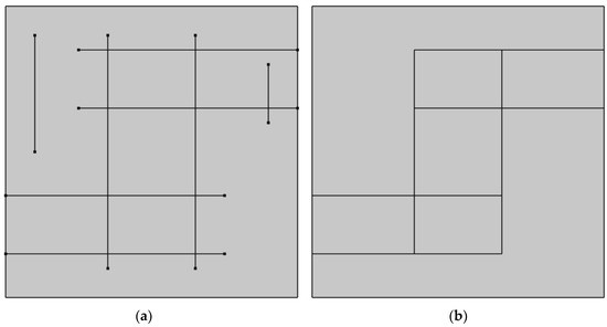
Figure 1.
An original fracture network and the extracted backbone fracture network: (a) Original network. (b) Backbone network.
The permeability mapping in the next section is based on the backbone network, because the fractures that are not connected to each other are able to be connected in permeability mapping due to the dead end or disconnected fracture, which cause a higher permeability. Using the backbone network can largely avoid the higher permeability and retain the effect of the fracture on seepage.
2.1.2. Permeability Mapping Approach
The permeability mapping method is proposed in Ref [35]. An analytical method is used to calculate the permeability of each sub-grid. The permeability of the model in this work is expressed in tensor to preserve the effect of fracture direction on fluid flow. For a fracture with an angle to the x-axis, the permeability tensor of the fracture in the two-dimensional coordinate system can be expressed as:
where is the angle between the fracture and the x-axis; is the permeability of the fracture. The contribution of the fracture to the hydraulic conductivity of the sub-grid, which is crossed, can be estimated as [36], where is the hydraulic conductivity of the fracture and is the size of sub-grid. The relationship of the fracture to the permeability of the sub-grid, which the fracture passes through, can be expressed as:
where is the permeability contribution of fracture to the sub-grid; and is the width of the fracture. Therefore, the permeability of each sub-grid can be calculated as:
where is the permeability of sub-grid(i, j); and is the permeability of matrix. For cases where multiple fractures pass through the same sub-grid, the permeability sub-grid can be calculated as follows:
where is the number of fractures passing through the sub-grid(i, j); and is the permeability of the sub-grid(i, j). Figure 2 shows the process of fracture permeability mapping.
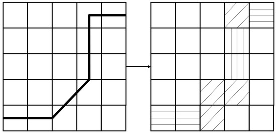
Figure 2.
The schematic diagram of permeability mapping.
Considering the error between the FCM model obtained after mapping and the DFN model, the permeability of FCM needs to be corrected as follows:
where is the corrected permeability of the sub-grid(i, j); C is the permeability correction factor used to correct for the error in flow rate that occurs from mapping. In Ref [36] research C is calculated as . In this work, the correction factor was calculated from the flow ratio between the DFN model and FCM model with uncorrected permeability.
2.2. Governing Equation
The fluid flowing in the thermal reservoir is described by Darcy’s law. The mass balance equation in the porous media is as follows:
where is the porosity of the rock matrix; is the density of the fluid; is the time; is the Darcy velocity; is the storage coefficient; is the pressure; is the permeability of media; is the fluid dynamic viscosity; is the source-sink term.
In this work, the local thermal non-equilibrium theory is used to describe the heat exchange between the rock and the fluid flowing in the geothermal reservoir. The energy balance equations are as follows [37,38]:
where is the density of the matrix; and are the temperatures of the matrix and fluid respectively; and are the specific heat capacities of the matrix and fluid respectively; and are the matrix and fluid thermal conductivities respectively; is the interstitial convective heat transfer coefficient.
In Section 3 of this paper, the permeability of the FCM model needs to be corrected by using the results of the DFN model. The governing equations in the matrix are the same as that used in the FCM model.
The mass conservation equation in discrete fractures is written as:
where is the Darcy velocity in the fracture. The porosity of fractures is assumed to be 100%, so the temperature of the rock is not considered in the energy balance equation of fractures. The energy balance equation for the fluid in the discrete fractures is written as [39]:
where is the temperature of the fluid in fractures; is a source term to describe the heat transfer between the matrix and fractures, which mainly results from the heat convection.
2.3. Well-Placement Optimization of EGS FCM Model
Generally speaking, there are two principles in EGS well-placement design [30]: longer major flow path and less preferential flow. However, it is difficult to find a long major flow path directly without preferential or short-circuit flow which is a notorious issue annoying EGS researchers and engineers [40]. Combinations of optimization algorithms and numerical simulations provide an idea for solving this problem.
2.3.1. Well-Placement Optimization Problem with 0-1 Programming
When designing an EGS well-placement, all wells, including injection wells and production wells, should pass through fractures because of the low permeability of the matrix. In the FCM model used in this paper, the thermal reservoir is divided into several equal-sized sub-grids, the parameters of each sub-grid represent the fractures’ effect to this sub-grid. Therefore, all wells are located in the fractured sub-grids that have high permeability, which can ensure adequate connectivity between wells and reduce the number of potential well-placements. As shown in Figure 3, there are just 36 potential well-placements in a FCM model with 100 sub-grids.
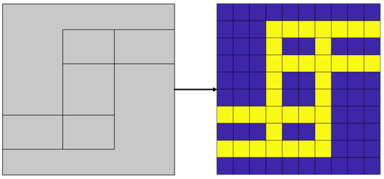
Figure 3.
Schematic diagram of high permeability grid mapping from the fracture network.
However, this method of well-placement designing would bring some difficulties to the optimization. Complex fracture distribution in the reservoir results in uneven distribution of high permeability sub-grids, which makes it hard to deal with the constraints of well-placement. Transforming the well-placement optimization problem into a 0-1 programming problem can solve this difficulty.
In this work, the well-placement optimization problem of EGS is considered as a 0-1 programming problem. The one-well injection and multi-well production pattern are applied in this work. All wells are located in the high-permeability sub-grid and only one well at most on each sub-grid. For each grid, the grid without the well is recorded as 0, and the grid where the well is located in is recorded as 1. The coding form is shown in Figure 4, where the yellow grids represent the high-permeability sub-grids and the blue grids represent the low-permeability sub-grids.
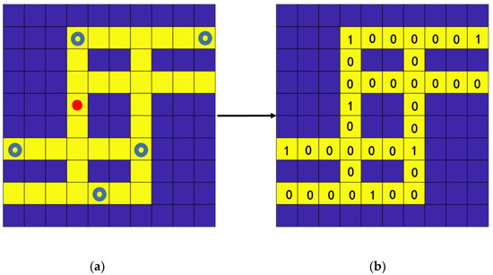
Figure 4.
The well-placement and the optimal variables (a) The locations of wells (red point represents injection wells and blue represents production wells). (b) The optimal variables transformed from well locations.
This gives variables consisting of 0-1 to indicate the number and location of wells in the thermal reservoir. The high-permeability sub-grids have been numbered and the well-placement would be transferred to a one-dimensional vector consisting of binaries. The injection wells and production wells are not distinguished in coding, but the well closest to the center of the model is used as the injection well, and the other wells are used as production wells. The EGS well-placement problem based on 0-1 programming can be described as follows:
where is a vector of 0s and 1s transformed from well-placement, is the objective function, is the upper limit of the number of wells, and is the lower limit of the number of wells.
2.3.2. Genetic Algorithm
In this work, a GA is used to solve the EGS well-placement optimization problem. A GA is an optimization algorithm that searches for the best solution by simulating natural evolution. The iteration of a GA begins with a population of individuals. One individual represents a potential solution and the population represents a potential set of solutions to a problem. The individual is encoded by genes that represent the variables of the problem. The individual is evaluated by the fitness value determined by the user. The fitness value is the result of the objective function in most cases. The process of population regeneration consists of selection, crossover, and mutation. The role of selection is to eliminate individuals with low fitness, and crossover and mutation are used to generate new solutions to keep the diversity of the population. The best individual in the last generation is seen as the approximate optimal solution to the problem.
The strategies in GA adopted in this work are given below:
- Initialization: N individuals are randomly generated before iterations, which is used as the first generation in GA.
- Fitness calculation: the fitness (objective function) of each individual is calculated by a numerical simulation.
- Selection: roulette is used to select parent individuals from the current population, which means that individuals with greater fitness are more likely to be selected, and the selected individuals enter the parents pool.
- Crossover: do the single-point crossover of individuals in the parent pool based on crossover probability.
- Mutation: single-point mutation is employed to make small random changes in the individuals in the parent pool
- Elitist strategy: an elitist strategy is applied in the process of evolution. The individual with the best fitness in the current generation is retained to the next generation without crossover and mutation.
- Stopping criteria: when the number of generations achieves the pre-set value, GA will stop.
- Constraint: the constraint in this work is the number of wells. The first generation is initialized in the feasible region, and the infeasible solution generated in the iteration will be repaired.
- Repair method: the production well closest to the center would be removed if the number of wells is above the upper bound of the number of wells, and the well would be added at random locations if the number of wells is below the lower bound.
The GA is written in MATLAB R2018b which is easy to combine with numerical simulation modules.
3. A Well-Placement Optimization Case
3.1. Computational Model
Natural fractures [41] or hydraulic fracturing fractures [42] in the reservoir can often be obtained from history matching or seismic inversion [43]. In this work, an assumptive model sized 200 m × 200 m is used as the original fracture network and the parameters of fractures are referenced from Ref [35]. Two hundred fractures, which are divided into two sets with different dip angles (i.e., 0° and 90°), are generated, and the fractures’ lengths follow exponent distribution with the maximum length of 200 m, the minimum length of 20 m and exponent of 1. The backbone of the generated network is extracted using the method described in Section 2.1.1. The thickness of the permeable layer is 10 m. Figure 5 shows the original fracture network and the backbone network.
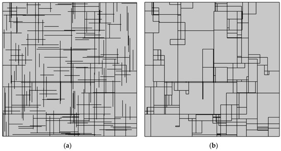
Figure 5.
Fracture network: (a) original network (b) backbone network.
The model is divided into 20 × 20 square sub-grids with a side length of 10 m. The permeability mapping is based on the backbone network shown in Figure 5b. There is no permeability heterogeneity on the x-y and y-x components due to the direction of the fractures. The x-x component and y-y component of the permeability tensor are shown in Figure 6.
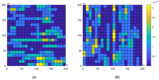
Figure 6.
The permeability tensor (mm2) of the FCM model. (a) x-x component (b) y-y component.
The mathematical model of the above governing equations including the matrix and fracture are discretized using the finite element method (the initial and boundary conditions are given in Section 3.2), which is solved using a commercial finite element software COMSOL Multiphysics 5.3 (COMSOL Co. Ltd., Stockholm, Sweden) and the GA written by MATLAB R2018b is linked to the software by LiveLink for MATLAB, which is developed by COMSOL. The parameters of GA are shown in Table 1.

Table 1.
The parameters of genetic algorithm (GA).
3.2. Model Parameters
The reservoir is initially saturated with water. All wells, including 4 production wells and 1 injection well work under constant pressure conditions. The working fluid for heat extracting is also water. The parameters are written in Table 2, which are referenced from some previous numerical studies [44,45]. The permeability of FCM has been corrected by the flow ratio of the DFN model and uncorrected FCM model.
Table 2.
Model Parameters.
No-flow and adiabatic boundaries are around the reservoir. The adiabatic boundary is set to better observe the effect of well-placement on heat extraction in temperature distribution. The initial and boundary conditions can be found in Table 3.
Table 3.
Initial and Boundary Conditions.
In this work, we just consider a five-spot well-placement pattern with one injection well and four production wells. The injection well and production wells are not distinguished in the 0-1 code. The well closest to the center of the model would be used as an injection well while the other wells would be used as production wells. To facilitate analysis of single well performance, the production well number would be numbered clockwise from the well that is closest to that production well (0,0).
3.3. Objective Function
In this work, accumulative extracted thermal energy is used as the objective function of the well-placement optimization. Considering the adiabatic boundaries, it is equal to the decline in the thermal energy of the reservoir. It is expressed as follow [45]:
where is the decline in thermal energy in the reservoir; is the initial temperature; and is the reservoir temperature in time .
Besides , the flow rate (), the accumulative extracted thermal energy (), the average production temperature () and output thermal power () are also used to evaluate the performance of a geothermal reservoir with different well-placement. , , and are defined as:
where is the length of the boundary of the well; is the accumulative extracted thermal energy; is the simulation time; is the average temperature of production water; is the temperature of injection water; and is the length of the outlet boundary.
3.4. Results and Discussion
Genetic algorithms do not require a given initial solution, which is different from traditional optimization algorithms. Therefore, two different five-spot injection/production patterns (named Case 1 and Case 2) are used as two comparisons of the optimization result. As in Section 2.3, the yellow grids represent the high-permeability sub-grids and the blue grids represent the low-permeability sub-grids. In Case 1 the production well 1 and 3 is located on a sub-grid without fractures, while in Case 2 all wells are set in the sub-grids passed through fractures just like the optimization result. Figure 7 shows the comparisons and the optimization result (named Case 3).
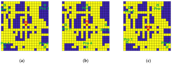
Figure 7.
The well-placement of two comparisons and the optimization result (the green circle represents the production well and the red circle represents the injection well): (a) Case 1; (b) Case 2; (c) Case 3.
Figure 8 and Figure 9 show the best individual of four different generations and the convergence process of the objective function. In Figure 9, the solid blue line indicates the best fitness in each generation, and the orange dotted lines indicate the average fitness of each generation.

Figure 8.
The best individual in (a) 1st generation (b) 10th generation (c) 20th generation (d) 40th generation.
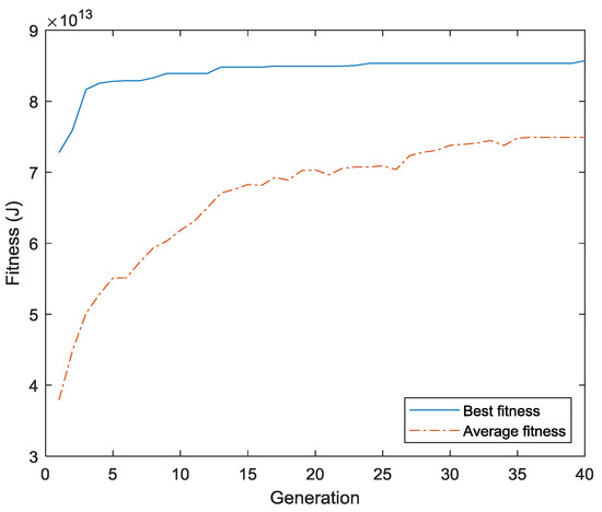
Figure 9.
The convergence process of the GA in well-placement optimization.
The convergence process shows that the best fitness achieved a high value in previous generations, which may be due to the fact that the wells are always placed in a high-permeability sub-grid during the optimization process. The lower average fitness in previous generations illustrates that many low fitness individuals are generated during the population initialization and genetic manipulation of previous generations, and the rapid increase in average fitness indicates that the entire population is evolving, which can prove the validity of 0-1 programming and GA in geothermal well-placement optimization.
The temperature variations of three cases are shown in Figure 10. The distribution of temperature is similar to each other at first because of the near location of the injection well. Gradually the cold front of each case migrates with the high-permeability sub-grid and the placement of production wells. It is obvious that the migrations of the cold front in Case 2 and Case 3 are faster than Case 1. The cold front in Case 1 only migrated to the Pro2 and Pro4 that are located in high-permeability sub-grids caused by the connected fracture. From the temperature variation, it can be observed that the effect of fractures to seepage and heat extraction is preserved in the FCM model.
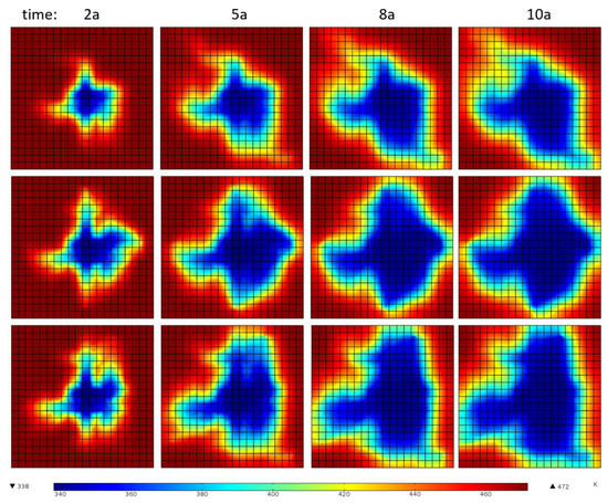
Figure 10.
The temperature variations of three cases. The top is Case 1, the middle is Case 2 and the bottom is Case 3 (optimization result).
The difference in heat extraction between Case 2 and Case 3 is not as obvious as between Case 1 and other cases, but it can be found that the temperature of the northeast in Case 3 is lower than Case 2 and the low-temperature region in Case 3 is larger than Case 2 overall. Considering that there is no supply source, the heat extraction in Case 3 is more adequate. The accumulative extracted thermal energy of the three cases are plotted in Figure 11.
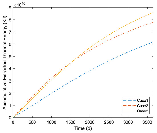
Figure 11.
The accumulative extracted thermal energy in the three cases.
As shown in Figure 11, the final of Case 3 from GA is higher than the two five-spot patterns that set to compare, which can also prove the validity of the well-placement method applied in this work. It also can be found that the heat recovery rate of Case 2 is higher than that of Case 3 in the first 1500 days. Figure 12 shows the change in output thermal power in the three cases, which is consistent with Figure 11. As shown in Figure 12, the power of Case 2 is highest in the first 700 days, but it also has the fastest decline. After 2500 days, the power of Case 2 is the least in all three cases.
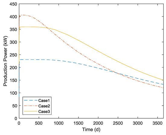
Figure 12.
The production power in the three cases.
At the initial running stage, the higher heat recovery rate indicates a better flow connection between the production well and the injection well, which means there are more fractures connected with the production well and injection well, but it does not mean the final performance will be better. Preferential or short-circuit flow in the thermal reservoir is always a headache for geothermal development and management. High flow velocity may cause a rapid decrease in matrix temperatures beside the connected fractures, which decrease the efficiency of heat convection. The average temperature shown in Figure 13 and the flow rate shown in Figure 14 can prove it.
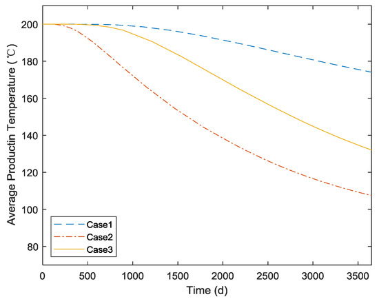
Figure 13.
The average production temperature of the three cases.
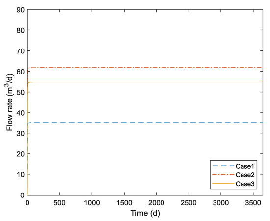
Figure 14.
The production flow rate of the three cases.
The flow rate is rapidly stable because of the little storage coefficient. As shown in Figure 13, the average production temperature of Case 2 has a fast drop. It can be inferred from the temperature and flow rate that the preferential flow exists in Case 2.
Figure 15, Figure 16 and Figure 17 show the accumulative energy, average temperature and the flow rate of each production well in the three cases. Consistent with the temperature distribution, the production wells, Pro1 and Pro3 in Case 1 contribute little to heat extraction, and the of Pro3 shows the preferential flow in Case 2 mainly exists between the injection well and Pro3, and the optimization result has been improved in it.
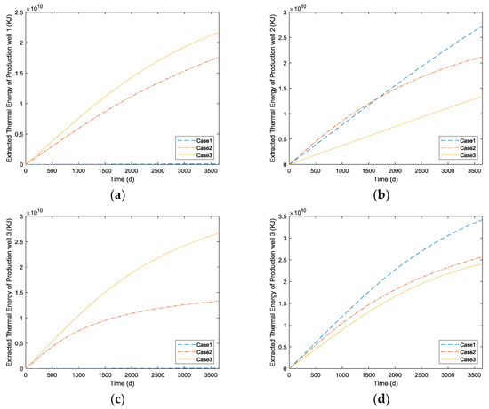
Figure 15.
The accumulative extracted thermal energy of the production well (a) Pro1 (b) Pro2 (c) Pro3 (d) Pro4.
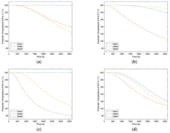
Figure 16.
The average temperature of the production well (a) Pro1 (b) Pro2 (c) Pro3 (d) Pro4.
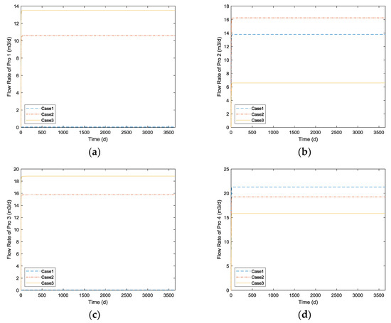
Figure 17.
The flow rate of the production well (a) Pro1 (b) Pro2 (c) Pro3 (d) Pro4.
4. Conclusions and Future Work
A well-placement optimization framework is proposed in this paper. FCM is used to simplify the fractured thermal reservoir model and the GA is used to solve the well-placement optimization problem that was considered as a 0-1 programming problem.
- The developed framework is efficient in the EGS well-placement optimization problem. The extracted thermal energy, which was the objective function, has increased in the convergence process of GA. And the optimization result shows better performance than comparison.
- The FCM model can reflect the effect of fractures on seepage and heat transfer to a certain extent.
- Regarding the well-placement optimization problem as a 0-1 programming problem can reduce the potential well-placements and improve the optimization effect. It also has the potential in joint optimization for well-placement and the number of wells.
- In the well-placement design of EGS, the connectivity between the injection well and production well should be considered as the primary factor. The well in low-permeability contributes little to heat extraction.
- Strong connectivity between wells does not mean better performance. Strong connectivity may lead to preferential flow and early heat breakthrough.
In this study, the framework only includes the 2-D model and the vertical well. In the future, this work will be generalized to the 3-D multi-field coupling model, a horizontal well, and the joint optimization of well-placement and the number of wells. A more advanced algorithm will be applied in EGS well-placement optimization, such as multi-objective optimization [46] and machine learning [47].
Author Contributions
Conceptualization, L.Z., Z.D. and K.Z.; Data curation, Z.D.; Formal analysis, L.Z. and T.L.; Funding acquisition, K.Z.; Methodology, L.Z. and K.Z.; Project administration, K.Z.; Software, Z.D.; Supervision, K.Z.; Validation, L.Z. and T.L.; Writing—original draft, Z.D.; Writing—review & editing, J.K.D., H.S. and Y.Y.
Funding
This work is supported by the National Natural Science Foundation of China under Grant 51722406, 61573018, 51874335 and 51674280, the Natural Science Foundation of Shan Dong Province under Grant JQ201808, the Key Research and Development Plan of Shan Dong Province under Grant 2018GSF116009, the National Science and Technology Major Project of China under Grant 2016ZX05025001-006, the Fundamental Research Funds for the Central Universities under Grant 18CX02097A, 17CX05002A and 17CX05003.
Conflicts of Interest
The authors declare no conflict of interest.
Nomenclature
The following terms are used in this manuscript:
| fracture permeability tensor (m2) | |
| angle between the fracture and the x-axis (°) | |
| fracture permeability (m2) | |
| fracture hydraulic conductivity (m/s) | |
| sub-grid size in FCM model (m) | |
| permeability contribution of fracture to the sub-grid (m2) | |
| fracture width (m) | |
| sub-grid (i, j) permeability (m2) | |
| matrix permeability (m2) | |
| fracture numbers | |
| corrected permeability of sub-grid (i, j) (m2) | |
| permeability correction factor | |
| matrix porosity | |
| fluid density (kg/m3) | |
| time (s) | |
| Darcy velocity (m/s) | |
| matrix storage coefficient (1/Pa) | |
| pressure (Pa) | |
| porous media permeability (m2) | |
| fluid dynamic viscosity | |
| source-sink term (1/s) | |
| matrix density (kg/m3) | |
| matrix temperature (K) | |
| fluid temperature (K) | |
| matrix specific Heat capacity (J/kg/K) | |
| fluid specific heat capacity (J/kg/K) | |
| matrix thermal conductivity (W/m/K) | |
| fluid thermal conductivity (W/m/K) | |
| interstitial convective heat transfer coefficient (W/m3/K) | |
| Darcy velocity in Fracture (m/s) | |
| fluid temperature in fracture (K) | |
| The decline in thermal energy of the reservoir (J) | |
| accumulative extracted thermal energy (J) | |
| the length of the boundary of well (m) | |
| simulation runtime (s) | |
| mass flow rate in time t (m3/s) | |
| production water temperature In time T (K) | |
| injection water temperature (K) | |
| average production temperature (K) | |
| output thermal power (kW) | |
| length of the outlet boundary (m) |
References
- Massachusetts Institute of Technology. The Future of Geothermal Energy: Impact of Enhanced Geothermal Systems (EGS) on the United States in the 21st Century; MIT: Cambridge, MA, USA, 2006. [Google Scholar]
- Brown, D. The US hot dry rock program-20 years of experience in reservoir testing. In Proceedings of the World Geothermal Congress, Florence, Italy, 18–31 May 1995; pp. 2607–2611. [Google Scholar]
- Office of Energy Efficiency and Renewable Energy; Lasala, R. An Evaluation of Enhanced Geothermal Systems Technology; Department of Energy: Washington, DC, USA, 2009.
- Tenzer, H. Development of hot dry rock technology. Geo-Heat Cent. Q. Bull. 2001, 32, 14–22. [Google Scholar]
- Polski, Y.; Capuano, L.; Finger, J.; Huh, M.; Knudsen, S.; Chip, M.A.; Raymond, D.; Swanson, R. Enhanced Geothermal Systems (EGS) Well Construction Technology Evaluation Report; Department of Energy: Washington, DC, USA, 2006. [Google Scholar]
- Procesi, M.; Cantucci, B.; Buttinelli, M.; Armezzani, G.; Quattrocchi, F.; Boschi, E. Strategic use of the underground in an energy mix plan: Synergies among CO2, CH4 geological storage and geothermal energy. Latium Region case study (Central Italy). Appl. Energy 2013, 110, 104–131. [Google Scholar] [CrossRef]
- Gan, Q.; Elsworth, D.; Cai, J. Heat transfer in enhanced geothermal systems: Thermal-Hydro-Mechanical coupled modeling. In Petrophysical Characterization and Fluids Transport in Unconventional Reservoirs; Cai, J., Hu, X., Eds.; Elsevier: Amsterdam, The Netherlands, 2019; pp. 201–205. [Google Scholar]
- Qin, X.; Cai, J.; Xu, P.; Dai, S.; Gan, Q. A fractal model of effective thermal conductivity for porous media with various liquid saturation. Int. J. Heat Mass Trans. 2019, 128, 1149–1156. [Google Scholar] [CrossRef]
- Abuaisha, M.; Loret, B.; Eaton, D. Enhanced Geothermal Systems (EGS): Hydraulic fracturing in a thermo–poroelastic framework. J. Pet. Sci. Eng. 2016, 146, 1179–1191. [Google Scholar] [CrossRef]
- Bear, J.; Fel, L.G. A Phenomenological Approach to Modeling Transport in Porous Media. Transp. Porous Media 2012, 92, 649–665. [Google Scholar] [CrossRef]
- Pruess, K.A. Practical method for modeling fluid and heat flow in fractured porous media. SPE J. 1985, 25, 14–26. [Google Scholar] [CrossRef]
- Yang, Y.; Liu, Z.; Sun, Z.; An, S.; Zhang, W.; Liu, P.; Yao, J.; Ma, J. Research on stress sensitivity of fractured carbonate reservoirs based on CT technology. Energies 2017, 10, 1833. [Google Scholar] [CrossRef]
- Ji, S.; Koh, Y. Appropriate Domain Size for Groundwater Flow Modeling with a Discrete Fracture Network Model. Groundwater 2017, 55, 51–62. [Google Scholar] [CrossRef]
- Neuman, S.P.; Depner, J.S. Use of variable-scale pressure test data to estimate the log hydraulic conductivity covariance and dispersivity of fractured granites near Oracle, Arizona. J. Hydrol. 2015, 102, 475–501. [Google Scholar] [CrossRef]
- Svensson, U. A continuum representation of fracture networks. Part I: Method and basic test cases. J. Hydrol. 2001, 250, 170–186. [Google Scholar] [CrossRef]
- Yang, Y.; Liu, Z.; Yao, J.; Zhang, L.; Ma, J.; Hejazi, S.; Luquot, L.; Ngarta, T. Flow simulation of artificially induced microfractures using digital rock and lattice Boltzmann methods. Energies 2018, 11, 2145. [Google Scholar] [CrossRef]
- Feyen, L.; Gorelick, S.M. Framework to evaluate the worth of hydraulic conductivity data for optimal groundwater resources management in ecologically sensitive areas. Water Resour. Res. 2005, 41, 147–159. [Google Scholar] [CrossRef]
- Yang, Y.; Yao, J.; Wang, C.; Gao, Y.; Zhang, Q.; An, S.; Song, W. New pore space characterization method of shale matrix formation by considering organic and inorganic pores. J. Nat. Gas Sci. Eng. 2015, 27, 496–503. [Google Scholar] [CrossRef]
- Chen, B.; Reynolds, A.C. Optimal Control of ICV’s and Well Operating Conditions for the Water-Alternating-Gas Injection Process. J. Pet. Sci. Eng. 2016, 149, 623–640. [Google Scholar] [CrossRef]
- Zhang, K.; Li, G.; Reynolds, A.C.; Yao, J.; Zhang, L. Optimal well placement using an adjoint gradient. J. Pet. Sci. Eng. 2010, 73, 220–226. [Google Scholar] [CrossRef]
- Janiga, D.; Czarnota, R.; Stopa, J.; Paweł, W. Self-adapt reservoir clusterization method to enhance robustness of well placement optimization. J. Pet. Sci. Eng. 2019, 173, 37–52. [Google Scholar] [CrossRef]
- Zhang, K.; Zhang, W.; Zhang, L.; Yao, J.; Chen, Y.; Lu, R. A study on the construction and optimization of triangular adaptive well pattern. Comput. Geosci. 2014, 18, 139–156. [Google Scholar] [CrossRef]
- Zhang, K.; Zhang, H.; Zhang, L.; Li, P.; Zhang, X.; Yao, J. A new method for the construction and optimization of quadrangular adaptive well pattern. Comput. Geosci. 2017, 21, 499–518. [Google Scholar] [CrossRef]
- Volkov, O.; Bellout, M.C. Gradient-based constrained well placement optimization. J. Pet. Sci. Eng. 2018, 171, 1052–1066. [Google Scholar] [CrossRef]
- Zhang, L.; Zhang, K.; Chen, Y.; Li, M.; Yao, J.; Li, L.; Lee, J. Smart Well Pattern Optimization Using Gradient Algorithm. J. Energy Resour.-Technol. 2015, 138, 012901. [Google Scholar] [CrossRef]
- Guyaguler, B.; Horne, R.N. Uncertainty Assessment of Well Placement Optimization. In Proceedings of the SPE Annual Technical Conference and Exhibition, New Orleans, LA, USA, 30 September–3 October 2001. [Google Scholar]
- Jesmani, M.; Bellout, M.C.; Hanea, R.; Foss, B. Well placement optimization subject to realistic field development constraints. Comput. Geosci. 2016, 20, 1185–1209. [Google Scholar] [CrossRef]
- Zhang, K.; Chen, Y.; Zhang, L.; Yao, J.; Ni, W.; Wu, H.; Zhao, H.; Lee, J. Well pattern optimization using NEWUOA algorithm. J. Pet. Sci. Eng. 2015, 134, 257–272. [Google Scholar] [CrossRef]
- Akın, S.; Kok, M.V.; Uraz, I. Optimization of well placement geothermal reservoirs using artificial intelligence. Comput. Geosci. 2010, 36, 776–785. [Google Scholar] [CrossRef]
- Chen, J.; Jiang, F. Designing multi-well layout for enhanced geothermal system to better exploit hot dry rock geothermal energy. Renew. Energy 2015, 74, 37–48. [Google Scholar] [CrossRef]
- Chen, M.; Tompson, A.F.B.; Mellors, R.J.; Abdalla, O. An efficient optimization of well placement and control for a geothermal prospect under geological uncertainty. Appl. Energy 2015, 137, 352–363. [Google Scholar] [CrossRef]
- Wu, B.; Zhang, G.; Zhang, X.; Jeffrey, R.G.; Kear, G.; Zhao, T. Semi-analytical model for a geothermal system considering the effect of areal flow between dipole wells on heat extraction. Energy 2017, 138, 290–305. [Google Scholar] [CrossRef]
- Guo, X.; Song, H.; Killough, J.; Du, L.; Sun, P. Numerical investigation of the efficiency of emission reduction and heat extraction in a sedimentary geothermal reservoir: A case study of the Daming geothermal field in China. Environ. Sci. Pollut. Res. 2018, 25, 4690–4706. [Google Scholar] [CrossRef]
- Matthäi, S.K.; Belayneh, M. Fluid flow partitioning between fractures and a permeable rock matrix. Geophys. Res. Lett. 2004, 31, L07602. [Google Scholar] [CrossRef]
- Chen, B. Study on Numerical Methods for Coupled Fluid Flow and Heat Transfer in Fractured Rocks of Doublet System. Ph.D. Thesis, Tsinghua University, Beijing, China, 2009. (In Chinese). [Google Scholar]
- Botros, F.E.; Hassan, A.E.; Reeves, D.M.; Pohll, G. On mapping fracture networks onto continuum. Water Resour. Res. 2008, 44, 134–143. [Google Scholar] [CrossRef]
- Xu, C.; Dowd, P.A. Zhao, F.T. A simplified coupled hydro-thermal model for enhanced geothermal systems. Appl. Energy 2015, 140, 135–145. [Google Scholar] [CrossRef]
- Saeid, S.; Al-Khoury, R.; Barends, F. An efficient computational model for deep low-enthalpy geothermal systems. Comput. Geosci. 2013, 51, 400–409. [Google Scholar] [CrossRef]
- Chen, B.; Song, E.; Cheng, X. Plane-Symmetrical Simulation of Flow and Heat Transport in Fractured Geological Media: A Discrete Fracture Model with Comsol. In Multiphysical Testing of Soils and Shales; Laloui, L., Ferrari, A., Eds.; Proceeding of Springer Series in Geomechanics and Geoengineering; Springer: Berlin/Heidelberg, Germany, 2013. [Google Scholar]
- Tenma, N.; Yamaguchi, T.; Zyvoloski, G. The Hijiori hot dry rock test site, Japan: Evaluation and optimization of heat extraction from a two-layered reservoir. Geothermics 2008, 37, 19–52. [Google Scholar] [CrossRef]
- Zhang, L.; Cui, C.; Ma, X.; Sun, Z.; Liu, F.; Zhang, K. A Fractal Discrete Fracture Network Model for History Matching of Naturally Fractured Reservoirs. Fractals 2019, 27, 1940008. [Google Scholar]
- Zhang, K.; Ma, X.; Li, Y.; Wu, H.; Cui, C.; Zhang, X.; Zhang, H.; Yao, J. Parameter prediction of hydraulic fracture for tight reservoir based on micro-seismic and history matching. Fractals 2018, 26, 1840009. [Google Scholar] [CrossRef]
- Zhang, K.; Guo, Y.; Zhang, B.; Trumbo, A.M.; Marfurt, J.K. Seismic azimuthal anisotropy analysis after hydraulic fracturing. Interpretation 2013, 1, SB27–SB36. [Google Scholar] [CrossRef]
- Sun, Z.; Zhang, X.; Xu, Y.; Yao, J.; Wang, H.; Lv, S.; Sun, Z.; Huang, Y.; Cai, M.; Huang, X. Numerical simulation of the heat extraction in EGS with thermal-hydraulic-mechanical coupling method based on discrete fractures model. Energy 2017, 120, 20–33. [Google Scholar] [CrossRef]
- Song, X.; Shi, Y.; Li, G.; Yang, R.; Wang, G.; Zheng, R.; Li, J.; Lyu, Z. Numerical simulation of heat extraction performance in enhanced geothermal system with multilateral wells. Appl. Energy 2018, 218, 325–337. [Google Scholar] [CrossRef]
- Zhang, L.; Wang, S.; Zhang, K.; Sun, Z.; Zhang, X.; Zhang, H.; Chipecane, M.T.; Yao, J. Cooperative Artificial Bee Colony Algorithm with Multiple Populations for Interval Multi-Objective Optimization Problems. IEEE Trans. Fuzzy Syst. 2018. [Google Scholar] [CrossRef]
- Wang, J.; Xu, C.; Yang, X.; Zurada, J.M. A Novel Pruning Algorithm for Smoothing Feedforward Neural Networks Based on Group Lasso Method. IEEE Trans. Neural Netw. Learn. Syst. 2018, 29, 2012–2024. [Google Scholar] [CrossRef] [PubMed]
© 2019 by the authors. Licensee MDPI, Basel, Switzerland. This article is an open access article distributed under the terms and conditions of the Creative Commons Attribution (CC BY) license (http://creativecommons.org/licenses/by/4.0/).