Article

Multi-Objective Optimization of Energy Consumption and Surface Quality in Nanofluid SQCL Assisted Face Milling

1
College of Mechanical and Electrical Engineering, Nanjing University of Aeronautics and Astronautics, Nanjing 210016, China
2
Manufacturing Department, School of Aerospace, Transport and Manufacturing, Cranfield University, Cranfield, Bedfordshire, MK43 0AL, UK
3
Mechanical and Production Engineering, Ahsanullah University of Science and Technology, Dhaka 1208, Bangladesh
*
Author to whom correspondence should be addressed.
Energies 2019, 12(4), 710; https://doi.org/10.3390/en12040710
Submission received: 16 December 2018 / Revised: 4 February 2019 / Accepted: 17 February 2019 / Published: 21 February 2019
(This article belongs to the Special Issue Energy Efficiency of Manufacturing Processes and Systems)

Abstract

:
Considering the significance of improving the energy efficiency, surface quality and material removal quantity of machining processes, the present study is conducted in the form of an experimental investigation and a multi-objective optimization. The experiments were conducted by face milling AISI 1045 steel on a Computer Numerical Controlled (CNC) milling machine using a carbide cutting tool. The Cu-nano-fluid, dispersed in distilled water, was impinged in small quantity cooling lubrication (SQCL) spray applied to the cutting zone. The data of surface roughness and active cutting energy were measured while the material removal rate was calculated. A multi-objective optimization was performed by the integration of the Taguchi method, Grey Relational Analysis (GRA), and the Non-Dominated Sorting Genetic Algorithm (NSGA-II). The optimum results calculated were a cutting speed of 1200 rev/min, a feed rate of 320 mm/min, a depth of cut of 0.5 mm, and a width of cut of 15 mm. It was also endowed with a 20.7% reduction in energy consumption. Furthermore, the use of SQCL promoted sustainable manufacturing. The novelty of the work is in reducing energy consumption under nano fluid assisted machining while paying adequate attention to material removal quantity and the product’s surface quality.

1. Introduction

Recently, immoderate energy consumption has become one of the most severe problems in the manufacturing industry, and conserving energy has become a necessity for the industry. In manufacturing processes, machine tools are the primary energy consuming devices [1]. Gutowski et al. [2] have concluded that 14.8% of total energy was utilized during the material removal process. According to Newman, 6–40% of energy can be saved by choosing optimum cutting parameters, cutting tools and cutting paths [3]. Additionally, the energy consumption of machine tools is also associated with an increased environmental cost. Therefore, there is a dire need for the optimization of cutting parameters based on minimum energy criteria. Material removal rate, cutting force, tool life, surface roughness (SR), power and energy consumption are the responses measured during the milling process. However, the optimization of a single objective has many limitations. The conclusion of the above discussion is that this problem necessitates the need for a framework to optimize conflicting objectives simultaneously.
The manufacturing industry is facing a new challenge to reduce energy consumption due to the higher demand forenergy and increasing concerns regarding fossil fuel depletion [4]. However, more difficulties arise when reducing energy consumption without compromising on the surface quality of the product. In the machining process, the typical interactions between the cutting tool-work surface and the cutting tool-chip cause severe friction and intensive material deformation. Even, the harder cutting tool becomes worn due to an excessive mechanical load on the tool edges. Moreover, the thermal adversities caused by friction at the adjacent surfaces instigate unfavourability in machining. This unfavourability demeans the machining productivity and consumes higher amounts of energy. A significant portion of consumed power is lost due to friction during the cutting process [5].
Thermal upsetting at machining interfaces can be pacified by using cooling agents. Likewise, the effects of friction can be limited by employing lubricating agents. Owing to this fact, the use of cooling-lubricating agents in machining is widespread to date. However, the growing concerns for the environment and human health-related problems have forced manufacturers to look for an alternative as well as better cooling-lubrication modes [6,7,8].
Considering those aspects, for decades, the alternative mode of cooling-lubrication in machining has been the use of small droplets of agents under high air pressure so that the impinged sprays penetrate in between the interfaces. These droplets serve two functions: (i) they reduce friction by creating a thin film in between the material bodies [9], and (ii) they enhance heat dissipation by absorbing and removing heat from that zone [10]. This approach is reported in the literature under a number of different terms such as: small quantity cooling lubrication (SQCL), minimum quantity cooling lubrication (MQCL), minimum quantity lubrication (MQL), and near dry machining (NDM) etc., although the different terms exhibit slight differences in the way the cooling is delivered. Many research works show the positive sides of SQCL [11,12]. However, more advantages are gained when SQCL was applied using nano-fluids in suspension. The improved tribological properties of the nano-fluids themselves result in several other benefits in machining, such as a reduced coefficient of friction, lower cutting forces, improved surface finish, reduced cutting temperature, and lower tool wear associated with prolonged tool life.
The use of nanoparticles such as Cu, CuO, Al2O3, MoS2, SiO2, and diamond/graphite nanoparticles in the base fluids in the machining process under MQL conditions has become a new trend. However, in depth analysis of the application of water-based nano-fluids in the machining process is still a common research area [13]. Mintsa et al. [14] measured the thermal conductivity of alumina and copper oxide mixed in water (water-based nano-fluids). They showed that the effective thermal conductivity increased when increasing the particle volume fraction and when reducing the size of nanoparticles. In another study, Zhang et al. [15] also measured the effective thermal conductivity of distilled water based nanofluids. The results revealed that effective thermal conductivity increases with the increase of nanoparticle concentration. Lvet al. [16] utilized graphene oxide/silicon dioxide hybrid nanoparticle in water-based nano-fluids in evaluating the machining characteristics of MQL technology. Results revealed a significant reduction in the worn scar diameter (WSD) and the coefficient of friction (COF) using hybrid GO/SiO2 water-based MQL technology in the milling process.
Modern manufacturing aims at reducing energy consumption as well as achieving high quality within small timeframes [17]. The International Organization for Standardization is currently working on an ISO/DIS 14955 and ISO/DIS 50001 series which would assess the energy efficiency of machine tools and their environmental effects. Kara and Li [18] developed an empirical model to characterize the relationship between energy consumption and machining parameters and reached the apparent conclusion that specific energy consumption decreases when increasing the material removal rate. Abhang and Hameedullah [19] investigated the productivity and power consumption of machine tools in the turning of EN-31 steel. Results showed that when the tool nose radius, cutting speed, feed rate and depth of cut were at lower levels, less power was consumed by the machine tool. Bhattacharya et al. [20] performed experiments to study surface quality and power consumption during the high-speed machining of AISI 1045 steel. The cutting speed was found to be the most significant cutting parameter for both surface roughness and power consumption. However, all experiments were performed under dry cutting conditions. Camposeco-Negrete [21] optimized the cutting parameters for minimum energy consumption in the turning of AISI 6061. It was found that feed rate has the most significant effect on the surface roughness and energy consumption; lower values of feed rate resulted in better surface finish, but with higher energy consumption. Pusavec et al. [22] conducted many experiments in the dry, MQL, cryogenic and hybrid cooling assisted machining of nickel-based Inconel alloy 718. Cutting forces, power, tool life, material removal rate and cooling and lubrication performance were studied. The cooling and lubrication techniques were found useful for reducing cutting forces and improving tool life.
Velchevet al. [23] developed an approach for the optimization of cutting parameters for minimum energy in the turning process. A mathematical model was developed that considered the cutting parameters to express the direct energy consumption of machine tool. Kumar et al. [24] performed a multi-objective optimization by assigning different weights to energy consumption, surface quality, and productivity. The authors have concluded that the depth of cut and the use of radius were vital factors for analytical hierarchy process (AHP) and entropy weight methods respectively. Maruda et al. [25] studied the influence of cooling conditions on-chip formation and tool wear. The authors have concluded that the application of MQCL reduced cutting tool wear.
To conserve resources while maintaining improved machinability, there is a need for multiple objectives optimization using different algorithms. Grey relation algorithm (GRA) is one of the most efficient algorithms used for multi-objective optimization [26]. The GRA is based on a simple calculation, and it can provide an accurate analysis of small sample size. Moreover, it can assign variable weights to each response. It reduces complex multi-objective objective problems into a single object effectively and efficiently. Mia et al. [27] successfully employed a GRA method to optimize the cutting force and surface roughness in end milling under MQL conditions. On the other side, Deb et al. [28] proposed a fast and elitist heuristic method know as Non-dominated Sorting Genetic Algorithm NSGA-II; researchers have been successfully using the NSGA II to optimize machining parameters. Rao et al. [29] employed NSGA II for a multi-objective optimization for multiple machining processes. Then, Li et al. [30] reported the use of NSGA-II for the machining of Ti-6Al-4V alloy machining.
It is evident that the chip-tool interface endures friction, which requires lubrication and cooling. At the same time, energy reduction is a prime motto of the sustainable production system. For that reason, the whole machining system needs to be optimized considering multiple objectives. On the one hand, GRA cannot provide us with a Pareto front solution to find trade-off relationships. However, on the other hand, NSGA-II cannot provide information on a complex problem as a single characteristic. So, to overcome the drawbacks of each algorithm and to present a solution to a complex problem in detail, the multiple objectives are simultaneously optimized in this study using both a conventional method (GRA) as well as using a heuristic one (NSGA-II). Besides these aspects, other novelties include the use of Cu nano-fluid in distilled water and its use in the form of SQCL, reduction of energy consumption, and improvement of material removal rate.

2. Experimental Procedure

The face milling experiments were performed on a CNC machine tool (Carver 400M_RT) with a spindle power of 5.6 KW and a maximum rotation speed of 6000 rpm. AISI-1045 steel was used as work material. A three fluted carbide cutting tool with a diameter of 24 mm was used for machining. Figure 1 shows the schematic, experimental setup, and equipment used in measurements.
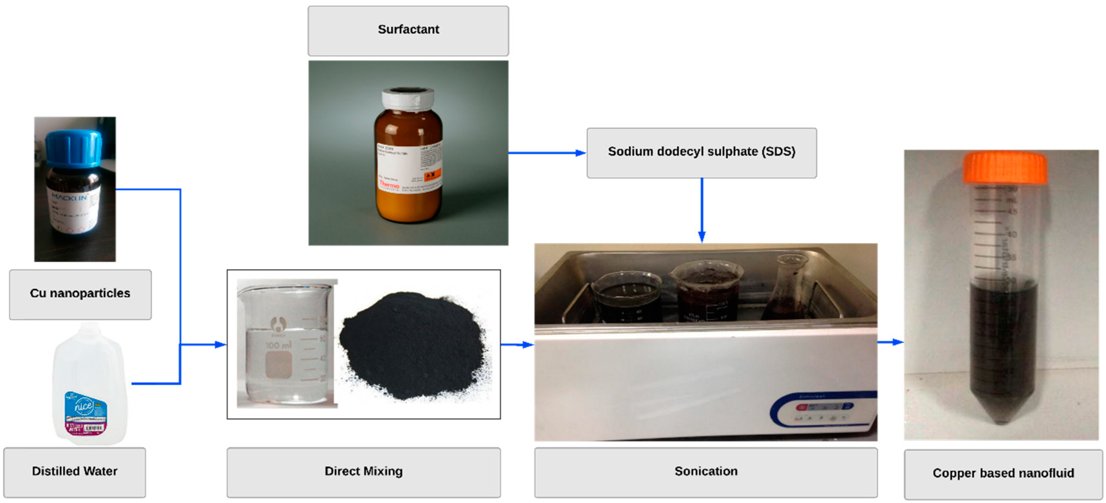
For nano-fluid based SQCL, a solution of copper nanoparticles suspended in distilled water was employed. Diionized water (DI water) was used as a coolant due to the fact that it has no harmful effects on workers’ health, and it is of low cost compared to other lubricants. Moreover, the addition of copper nanoparticles in distilled water increases its thermal stability, as reported by Mintsa et al. [14]. Copper nanoparticles with a 60 nm diameter were mixed with distilled water to prepare the solution (encouraged by reference [31]). The dispersion stability of nanoparticles is essential to investigate their performance. Thereby, the sodium dodecyl sulfate (SDS) was used as the surfactant in the mixture to achieve good stability. The stability mechanism of nano-fluid was measured in terms of zeta potential Z. Zeta potential values of more than 30 mV showed the high stability of the nano-fluid and its value was found to be positive 45 mV, depicting that the nano-fluid was highly stable. Figure 2 shows the preparation procedure of the Cu based nanofluid.
The focus of the study is to investigate the effect of cutting parameters on the responses above. Therefore, the technological parameters related to the SQCL system were kept constant by doing preliminary experiments and following the existing literature [11,12]. The nano-fluid SQCL was sprayed using a single nozzle at an air pressure of 4 bars, a lubricant flow rate of 300 mL/h; and a nozzle angle of 45°. The maximum material removal volume (MRV) was set to 2400 mm3. Experiments were designed according to the Taguchi L27 orthogonal array. Cutting parameters and their levels were selected by making preliminary trial runs and also from the published literature [32].
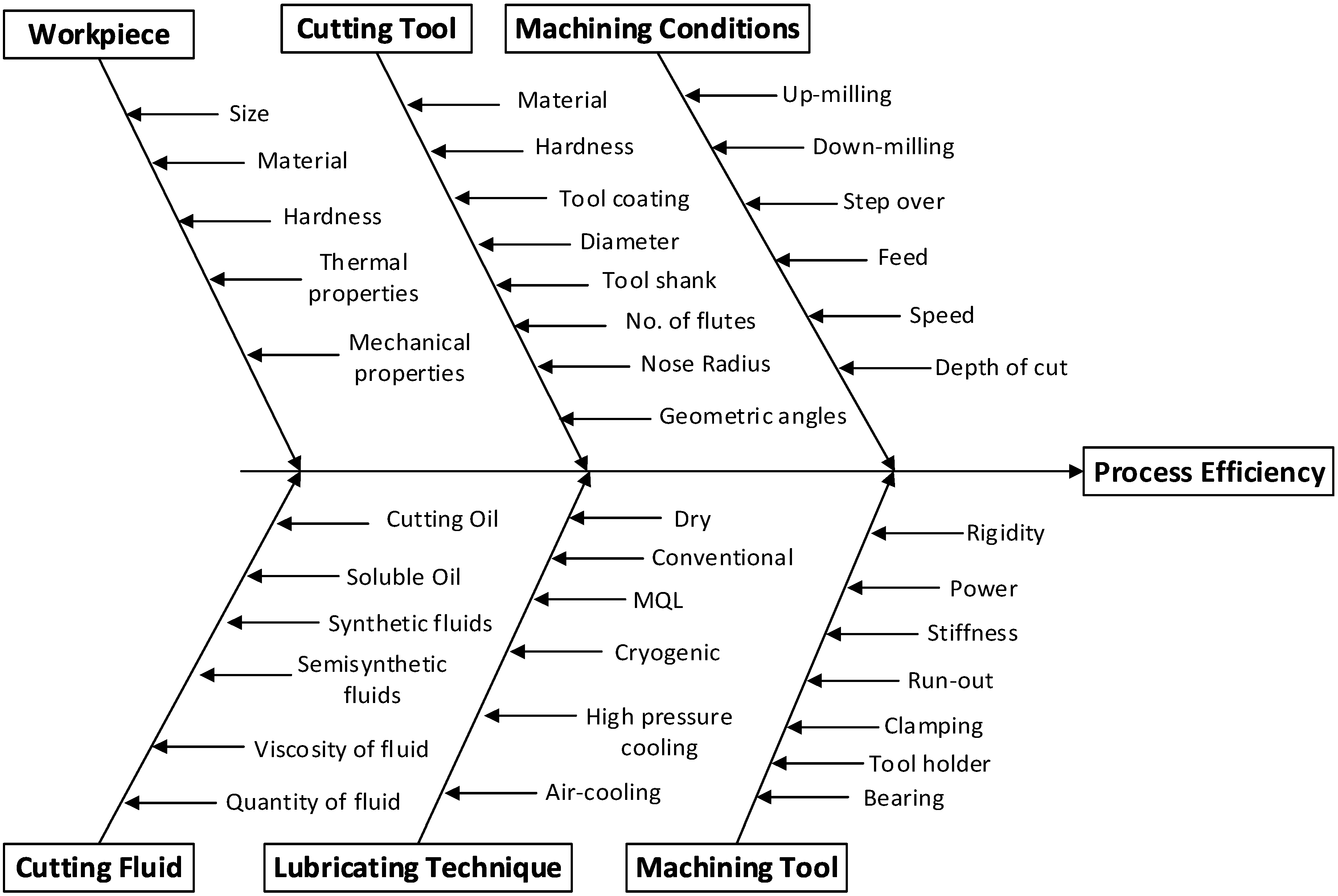
Figure 3 shows the cause-effect diagram for the efficiency of the machining process. In the current study, machining parameters (spindle speed, feed rate, depth of cut, and width of cut) were selected. Table 1 contains the levels of cutting parameters.

3. Response Measurements

The responses were measured for three successive runs, and finally, the average of the measured data was adopted as the mean value for further computation.

3.1. Production Rate

The production rate was determined by the material removal rate (mm3/min) which was computed using Equation (1) [32].
M R R = f z × z × N × a p × a e
where z , a p , a e are the number of tool flutes, depth of cut and width of cut, respectively.

3.2. Surface Quality

The quality of the produced machined surface was defined by the average of the roughness profile that the machining process was generating. For that purpose, the average surface roughness parameter (SR) was selected as the representative index of surface quality. It was measured using a portable stylus profilometer Mitutoyo Surftest SJ-410 at three equally separated points, and the average values were taken to mitigate errors [33].

3.3. Active Cutting Energy

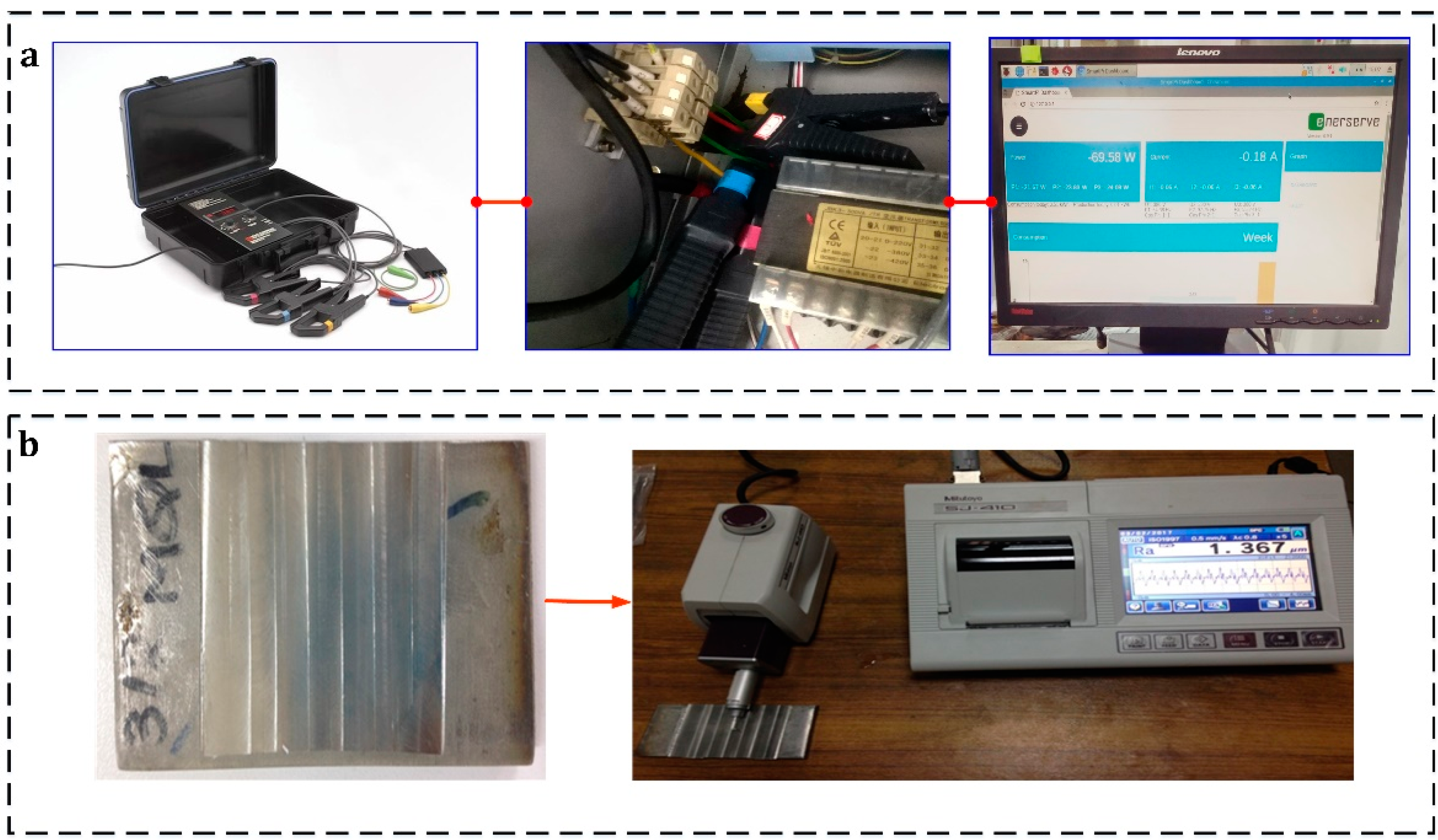
The Portable Power Cell model PPC-3 (Figure 4) was used to measure power demand during the cutting process. To measure the active energy consumption, a power sensor was attached to the main bus of the electrical cabinet of the CNC machine at a sampling frequency of 10Hz. Equation (2) can be used to estimate active energy consumption [32].
ACE = i = 1 k P i × t i 1000
where ACE ; active cutting energy (kJ), P i ; active power measured in watts (W), t i ; time, and k ; data samples during the process. In the experimental analysis, the lubricant delivery system used a separate power resource that was assumed to be constant. The measurement system for surface roughness and power consumption is shown in Figure 4.

4. Results and Discussion

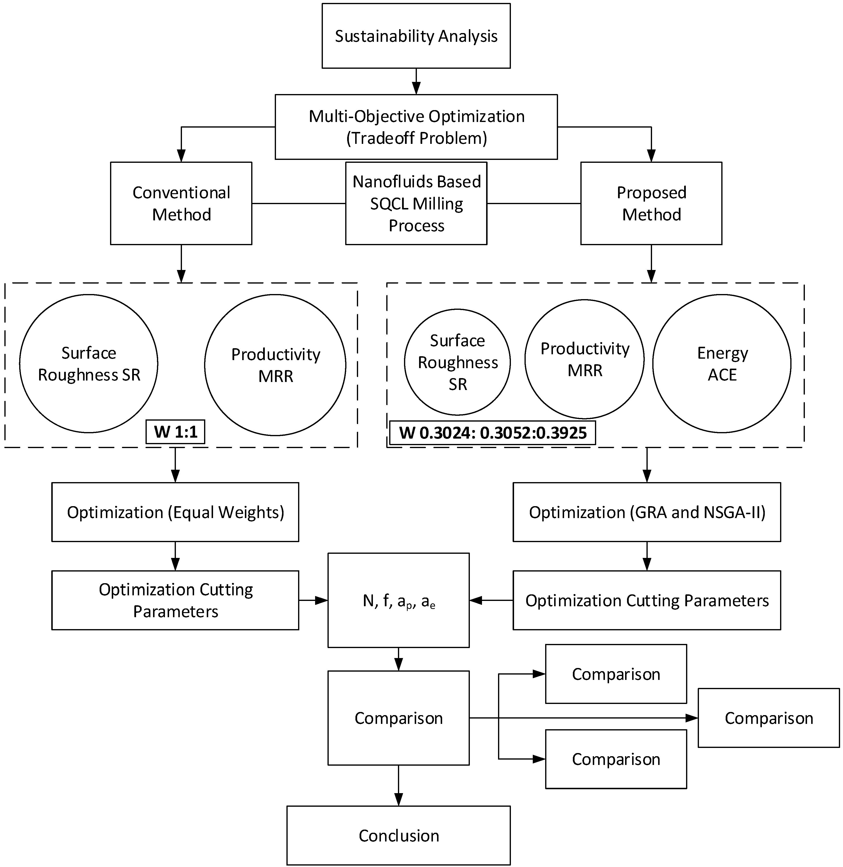
In this section, the multi-objective optimization is performed using Grey relational analysis (GRA) and NSGA-II methods to deal with difficult decision-making situations. Furthermore, the influence of the milling parameter on the surface quality, material removal rate and the cutting energy consumption is discussed. Finally, the mechanism of nano fluid assisted machining favorability is presented. The framework of the multi-objective optimization problem is shown in Figure 5. The framework explains the importance of energy consumption as a response. A comparison has been performed between the conventional method when only two responses (surface quality and productivity) are considered and a proposed method where energy is a sustainable parameter has been added. In the conventional method, equal weights are given to both responses to give them equal importance. However, in the proposed method an entropy method has been employed to the weights of each response according to the sensitivity of the response. In the proposed method, optimization has been performed using two algorithms: GRA and NSGA-II. The reason for employing both optimization algorisms is to get benefits from both methods to understand the complex multi-objective problem fully. The application of GRA is straight forward and quick. It converts the multi-objective optimization problem into a single objective and provides Grey relational grades (GRG).The GRG is a performance index of the GRA and provides information as a single characteristic in optimization problems. For example, a GRG value of 0.8678 highlights the best experiment in the L27 design. However, the heuristics are mostly recommended for the optimization instead of classic approaches, due to their capacity for a more precise global search. It is nearly impossible to get the optimal values of all responses simultaneously. So, NSGA-IIhas been used to obtain Pareto fronts to find the tradeoff relationships between a pair of two objects. GRA provides us the local optimal results. However, NSGA-II provides global optimal results.
Experimental design L27 along with process parameters and obtained results are presented in Table 2.

4.1. Grey Relational Analysis

Grey relational analysis was used to solve the complicated multi-objective optimization problem. There are three simple steps for this algorithm. In the first step, to avoid variability and different units, each response value was normalized. If the required objective is ‘the larger the better’, then the results were normalized using Equation (3). If the objective is ‘the smaller the better’, then the results were normalized using Equation (4) [26],
x i ( k ) = x i 0 ( k ) min ( x i 0 ( k ) ) max ( x i 0 ( k ) min ( x i 0 ( k ) )
x i ( k ) = max ( x i 0 ) x i 0 ( k ) max ( x i 0 ( k ) min ( x i 0 ( k ) )
The grey relation coefficients (GRC) for each factor were calculated by Equation (5). Finally, Grey relational grades (GRG) were computed using Equation (6) [26].
ξ ( k ) = Δ m i n + ξ Δ m a x Δ 0 i ( k ) + ξ Δ m a x
γ i = k = 1 n w k ξ i ( k )
Δ 0 i ( k ) is known as the deviation sequence and it is the absolute value. Minimum and maximum values of Δ 0 i ( k ) are denoted by Δ m i n and Δ m a x , respectively γ i represents the GRG of each experiment provided in Appendix A. The values of ξ lies between 0 and 1 and it is called a distinguishing coefficient, normally it is taken as 0.5. The w k represents the normalized weightage of factor k .
Traditionally, equal weights are assigned to objectives in simple problems. However, in complex problems, it is not easy to assume equal weights for each criterion. In complex multi-attribute decision making (MADM) problems, the weight of each criterion is calculatedby prioritization, expert opinion, and evaluation [34]. Finding an appropriate and effective way to assign the weights is a dire need of the MADM. Subjective and objective are the two well-known weight assignment methods. The examples of subjective weight assignment methods are the AHP, Delphi method, and weight least square method; in these methods, weights are assigned according to the preference of the decision makers.
Moreover, subjective weight methods are less accurate and have some drawbacks [35]. However, in the objective based weight assignment method, weights are assigned on the inherent information of indexes to determine weights of indexes. Entropy-based weight assignment is an objective weight assignment method which not only avoids human-made disturbances and assumptions but also provides results according to the sensitivity of the objectives. In that way, more realistic and accurate weights are calculated [35]. For these reasons, in this paper, the weight of each response was calculated in a systematic manner using entropy weighting.
In common practice, the concept of entropy is originated from thermo-science. This method finds the weight factor based on the influence of various input parameters on responses [24]. According to which, a higher weight should be assigned to the objective with higher variation in its values. In the first step, the mean values of each coefficient for each response were calculated based on Table 3. For example, to calculate the mean values of the Grey relation coefficients of the width of cut at cutting level 1 (5 mm), all experiments were selected with a width of cut at 5 mm and then the mean was taken.
Similarly, the mean was taken at level 2 (10 mm) and level 3 (15 mm), respectively. The range was calculated from the difference between the maximum and minimum values of the mean of GRC. The Ranges (R) for each factor were computed using Equation (7).
Ri,j = max{Qi,j,1, Qi,j,2, … Qi,j,s} − Min{Qi,j,1, Qi,j,2Qi,j,s}
w i = i = 1 c R i , j / i = 1 c j = 1 p R i , j
where, I = 1, 2, … c, c: number of response. j = 1, 2, … p , p : cutting parameters. s = 1, 2, … l, l: cutting parameter’s level. Similarly, R: GRC range, Q: mean Grey relational coefficient of each cutting parameter at three different levels (Appendix B).
Weights for each response were computed using Equation (8). Finally, Equation (9) was used to calculate grey relation grades and is given in Table 4.
GRG = 0.305 × GRC(MRR) + 0.302 × GRC(SR) + 0.392 × GRC(ACE)
GRC(MRR), GRC(SR), GRC(ACE) in Table 4 are the grey relation coefficients of material removal rate, surface roughness, and active cutting energy. GRG is an overall all Grey relation grade.

4.2. Development of RSM Models and Analysis of Variance

The second order Response Surface Methodology (RSM) models for the three objective functions: material removal rate, surface roughness, and active cutting energy were formulated using the measured data presented in Table 2. Process parameters in coded form affected the response more evenly, thereby accelerating the convergence speed of the algorithm and improving the precision of the algorithm. Coded variables were sometimes plotted on the x-axis and can easily be calculated by Equations (10)–(13).
A = ( N 1700 ) / 500   Coded   Variables = 1 ,   0 ,   1
B = ( f 270 ) / 50 Coded   Variables = 1 ,   0 ,   1
C = ( a p 0.4 ) / 0.1 Coded   Variables = 1 ,   0 ,   1
D = ( a e 10 ) / 5 Coded   Variables = 1 ,   0 ,   1
It is necessary to understand the relationship between cutting parameters and Grey relational grades forthe optimization of cutting parameters. Response surface methodology was employed to generate the second-order RSM model for MRR, SR, and ACE. Mia et al. [36] worked on the investigation of machinability characteristics and concluded that well-fitting mathematical models could be obtained using RSM. Equations (14)–(16) describe a second-order empirical model for MRR, SR, ACE respectively. Moreover, Equation (17) shows the mathematical relation of Grey relational grade regarding input parameters.
MRR(N,f,ap,ae) = 3048 − 1.45 × (N) − 3.15 × (f) − 10665 × (ap) + 51.3 × (ae) + 0.0002 × (N2) − 2.9 × 10⁻¹⁷ × (f2) + 6750 × (ap2) + 2.7 × (ae2) − 5.0 × 10⁻⁴ × (N × f) + 2.7 × (N × ap) − 0.054 × (N × ae) + 10.0 × (f × ap) + 0.4 × (f × ae)
SR(N,f,ap,ae) = − 8.9 − 5.56 × 10⁻⁴ × (N) + 0.043 × (f) + 37.67 × (ap) − 0.06 × (ae) + 1.0 × 10⁻⁶ × (N2) − 5.8 × 10⁻⁵ × (f2) − 32.44 × (ap2) + 0.015 × (ae2) − 5.16 × 10⁻⁶ × (N × f) − 0.007 × (N × ap) + 0.0001 × (N × ae) + 0.014 × (f × ap) − 3.53 × 10⁻⁴ × (f × ae)
ACE(N,f,ap,ae) = 2985.65 − 0.29 × (N) − 4.87 × (f) − 5911.40 × (ap) − 71.63 × (ae) + 5.4 × 10⁻⁵ × (N2) + 0.0036 × (f2) − 3794.33 × (ap2) + 2.67 × (ae2) − 3.12 × 10⁻⁵ (N × f) + 0.6535 × (N × ap) − 0.0133 × (N × ae) + 3.04 × (f × ap) + 0.083 × (f × ae)
GRG(N,f,ap,ae) = 0.895 − 0.00016 × (N) − 0.0015 × (f) + 1.91 × (ap) + 0.0057 × (ae) + 2.0 × 10⁻⁶ × (f2) + 1.17 × (ap2) + 0.0018 × (ae2) − 0.00002 × (f × N) + 0.00067 × (f × ap) + 0.00057 × (f × ae)
Figure 6 presents the relationship between the measured and predicted values of GRG. Measured values were close to predicted values, and the average percentage deviation was found to be 4.69, which indicated that experimental and predicted results were in good agreement.
Table 5 presents the analysis of variance (ANOVA) results for the regression model. ANOVA results illustrated that the coefficient of determination R-square value was 99.02%, and R-(adj) was 98.03%, which indicated the model’s excellent compatibility with experimental results. Experiment No. 9 (in bold in Table 4) was identified as the optimal trade-off having combination ( N = 1200 rev min ,   f = 320 mm min ,   a p = 0.5   mm ,   a e = 15   mm ) and can be verified from Figure 6 as having the highest GRG value.

4.3. Non-Dominated Sorting Genetic Algorithm NSGA-II

The genetic algorithm is a heuristic algorithm to optimize NP-hard problems inspired by a natural selection process in bio-science systems. Srinivas and Deb [37] proposed NSGA, and later Deb et al. [38] proposed NSGA-II, which elevates all the short-comings of NSGA, NSGA-II can obtain true Pareto optimal solutions based on the rank of non-domination. In NSGA-II, minimization of fitness is assumed, and each solution is given a rank which is equal to its non-domination level, e.g., one is considered the best level. Therefore, it obtains solutions not just within the experimental runs, but global space is used for searching for the optimal solution. A flowchart of GRA coupled with NSGA-II has been shown in Figure 7.
To convert multi-objective optimization into a single objective optimization problem, each objective function is multiplied with its respective weight. Improvement in the response highly depends on the weight assigned. In weight-based GA (WBGA), weights are random; this random assignment of weights does not consider the priority of responses. Therefore, the optimal solution is not guaranteed. In random weight assignment methods, weights are assigned to each objective function and then combined them to make a single objective. However, although these methods are simple to use, weight selection is still a challenging problem. In this paper, the weight of each response was calculated in a systematic manner using entropy weighting of GRA as discussed in Section 4.1.

4.3.1. Optimization Variables and Objective Function

Equations (14)–(16) serve as the objective function of NSGA-II. In this method, NSGA-II was the main technique, and GRA entropy was utilized to generate the weight of each response. NSGA-II was used to find four optimized milling parameters (spindle speed, feed rate, depth of cut, and width of cut) so that the best performance measures (MRR, SR, and ACE) were achieved without violating any of the constraints considered for this problem. For the simultaneous optimization of goals, the three objective functions were given as follows: Objective 1 = material removal rate; Objective 2 = surface roughness; Objective 3 = active cutting energy.

4.3.2. Constraints and Parameters for the NSGA-II Algorithm

The measured response must meet the constraints in the CNC milling process. Following the practical situation, the following constraints were considered.
Machine tool: CNC milling conditions must be within an allowable range of machine tool parameter values; Equation (18) explains this constraint for processing.
x m i n < x i < x m a x ( i = 1 , 2 , 3 , 4 )
P c = F c D n 318 < η P m a x
x i denotes milling parameters, Fc represents the maximum cutting force, P m a x is nominal motor power, and η themachine efficiency. In the optimization procedure using NSGA-II, the following parameters were listed based on the study to get optimal solutions with low computational effort and have been set by trial and error through many repeats of simulations and also determined from the literature [39]: crossover probability: 0.95; distribution index for the crossover: 10; mutation probability: 0.01; distribution index formulation: 10; population size: 100.

4.3.3. Pareto Optimal Front

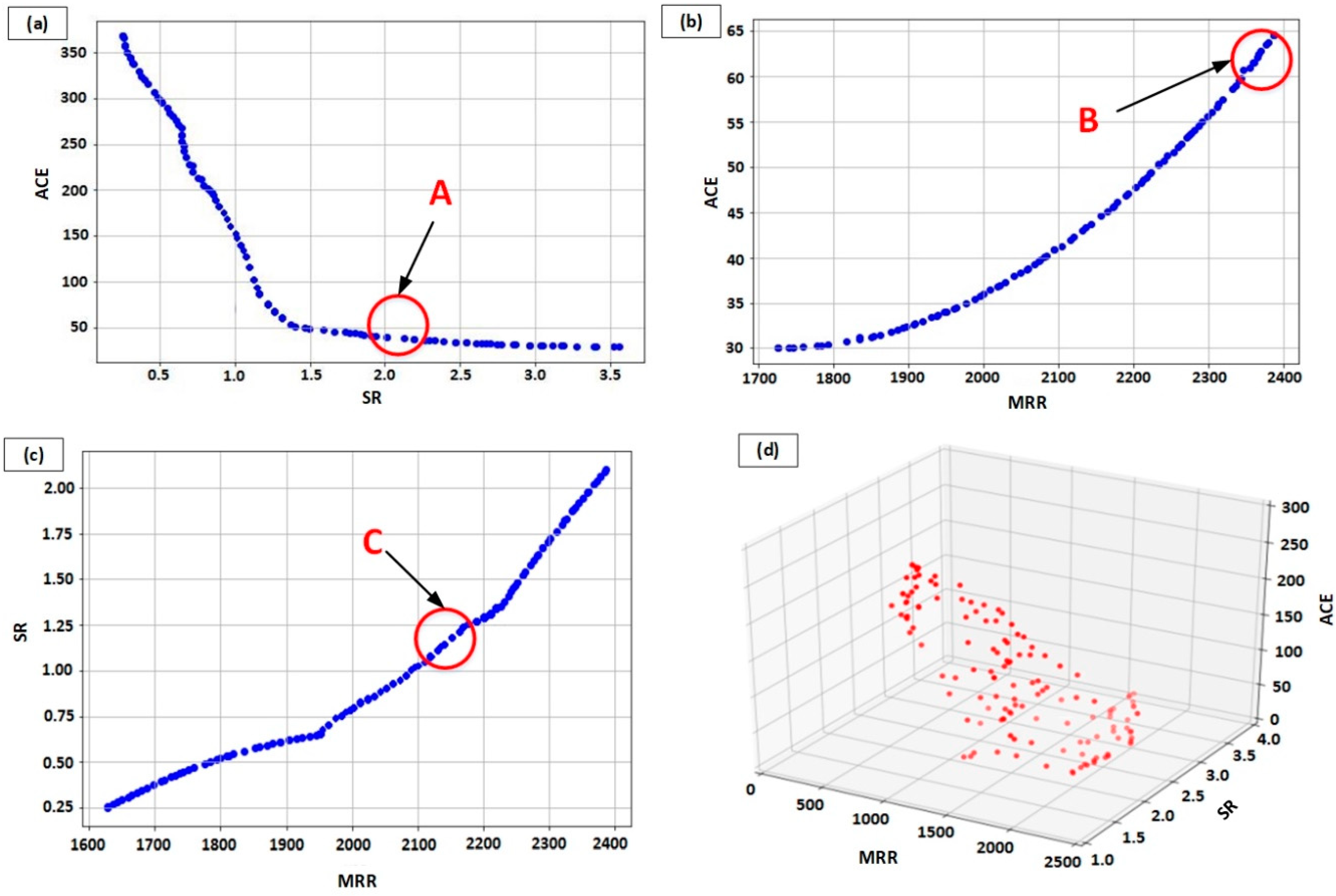
Pareto-optimal fronts were obtained from NSGA-II and are displayed in Figure 8. The data points in the Pareto-fronts do not dominate each other, and they represent the optimal combinations of milling parameters. The selection of any data points from Pareto fronts depended upon desired SQCL milling criterion. It is clear from Figure 8 the active energy consumption values decreased as the surface roughness increased.
However, ACE increased as the MRR increased. On the other hand, surface roughness values also increased as the MRR increased. As seen in Figure 8a, region A consisted of a Pareto-front solution, which was good for reducing ACE and at the same time not causing an increase in R a values. The optimized values of cutting parameters and response values were: (N:1622.38; f:300.394; ap:0.4999; ae:13.7012; SR:2.022; ACE:40.2928) at point A. In addition, the Pareto optimal solutions in region B were good for getting maximum productivity. However, the ACE was higher in this region. The optimized milling parameters at point B were: (N:1200; f:320; a p :0.5; a e :15) and the corresponding response values were: (MRR:2387.5; ACE:64.60). Similarly, point C was a tradeoff between SR and MRR with optimized milling parameters at point: (N:1217; f:320.001; a p :0.3; a e :15) and the response values were: (MRR:2135.73; SR:0.66). Besides, other solutions can be selected after considering the desired criteria. A wide range of Pareto-optimum solutions demonstrated the applicability of this method in machining optimization that considers conflicting objectives.

4.4. Influence of Milling Parameters on MRR, ACE, and SR

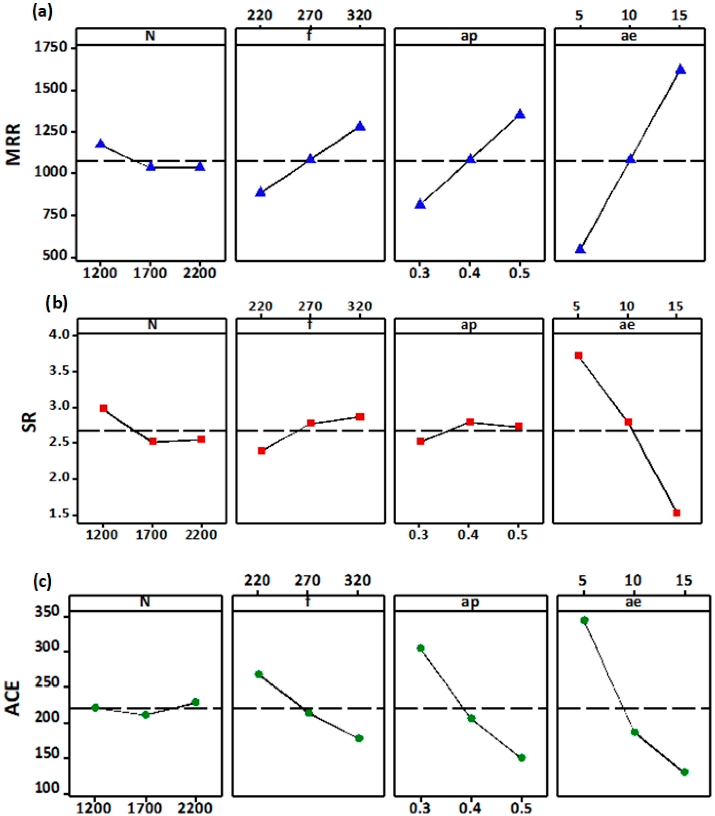
It is clear from Figure 9 that for active cutting energy (ACE) and MRR, the width of the cut had the most significant effect, while for spindle speed, this effect was the least significant.
Furthermore, GRC of ACE and MRR were in a linear relationship with the width of cut, so the highest value of the width of cut produced the lowest values of ACE and highest MRR. Similarly, for SR, the width of the cut also showed the most significant effect. From Table 2, the maximum SR values were found at a 5 mm width of cut, and the lowest SR value was found at 15 mm.
Extensive dispersion of Cu nanoparticles in the distilled water facilitated by cool high-pressure mist in workpiece and tool interface showed an excellent performance in reducing surface roughness. The mist from nano-fluid assisted SQCL systems exhibited more efficient feeding into the machining zone than the conventional cooling method [40]. This was because, in conventional wet cooling, lubricant splashes off by the rotating tool, but, mist sticks to the tool-workpiece interface and thus assists in improving cutting performance. In addition to this, the Cu nanoparticle in the SQCL provided a polishing effect, since an interacting force was then induced between the tool-particle interface, which is shown in Figure 9a [41]. This induced interacting force travelled upon the cutting tool interacting surface and produced power on the surface. Hence, the surface energy of the workpiece was significantly reduced due to a high interacting force between the particle workpiece interface [42].
On the one hand, the breaking of nanoparticles required a certain energy for the removal of asperities from the workpiece surface, which generated a new surface with better finish. On the other hand, the process of making Cu nanoparticles transferred potential energy from a cutting tool, which later became kinetic energy of workpiece surface atoms. Therefore, a 300 ml/h flow rate provided a number of Cu nanoparticles, which transferred more kinetic energy to surface atoms and enhanced heat dissipation from the cutting zone. Figure 9b explains how nanoparticles behave as a spacer and effectively minimize the frictional effects between interacting surfaces. In the high speed-milling process, heat generated in the cutting zone altered elasto-hydrodynamic lubrication into boundary lubrication, and thus, this may create a possibility of rolling effect (Figure 9b) which could result in a reduction in coefficient of friction [43].
Moreover, the increase in the concentration of Cu particles in distilled water strengthened the thin protective film on the workpiece surface. Thiswas due to the strong chemical interaction between the newly generated surface and nanoparticles. This phenomenon increased the surface quality of the workpiece [42]. The decrease in surface roughness was mainly due to the nanoparticles between the workpiece-tool interface. A good surface finish was mainly due to the excellent lubrication that slides the chips away from tool surface; better chip quality resulted in less surface roughness. Furthermore, a mist formation that entered the machining zone reduced the friction due to a ball bearing effect due to billions of rolling nanoparticles, and high-pressure spray removed the chips, ultimately leading to a better surface finish [44]. A higher concentration of solid fine Cu nanoparticles of a large size provided effective lubrication under aggravated sliding conditions. Because these particles easily penetrated the surface between rubbing face, the original sliding friction divided into sliding as well as rolling friction, and that reduced the coefficient of friction [45].

4.5. Comparative Analysis and Validation

Traditionally, specialized handbooks and worker experience are used to determine the desired cutting parameters, but these sources provide starting values of cutting parameters, and these values are not necessarily suitable for optimal conditions. Initially, the levels of milling parameters were set at (N2, f2, a p 1 ,   a e 1 ), and this combination is shown in Table 2 at experiment number 13. In this study, Figure 2 describes conventional multi-objective optimization, different from our purposed optimization method, only surface roughness, and material removal rate were selected as the optimization objectives in conventional optimization. Milling parameters (N = 2200 rev/min, f = 320 mm/min, a p = 0.5 mm and a e = 15 mm) were identified as the optimal setting for conventional multi-objective optimization. In order to perform the comparison between conventional and proposed multi-objective optimization method, we have also obtained optimal milling parameters from conventional optimization with two objectives. Table 6 shows the comparison of the experimental results of two optimization methods.
Initially, the GRA based optimization results compared with the initial settings of milling parameters. For the comparison of two methods, material removal volume (MRV) was fixed to the maximum level, i.e., 2400 mm3. As a result, SR and ACE decreased from 2.85 µm to 2.29 µm and 269.6 kJ to 53.98 kJ respectively. Parameters settings based on the proposed optimization method resulted in a 79.9% reduction in energy consumption as compared to the initial setting. It is clear that the proposed optimization method can improve multi-response in the cutting process. The feasibility of the proposed method is indicated by the promising results obtained.
As shown in Table 6, the GRA based optimization resulted in a 20.7% reduction in ACE as compared with conventional objectives optimization. Moreover, along with traditional objectives, the proposed method also added a sustainable objective, i.e., active energy consumption, which promotes environmental benefits and saves energy.

5. Conclusions

With an objective to simultaneously reduce the energy consumption and improve the surface quality, this study presented an experimental and optimization approach to reduce energy consumption and improve surface quality without compromising the material removal quantity under the use of nano-fluid assisted SQCL. The optimization was performed as a ‘multi-objective’ using GRA and NSGA-II methods. The following concluding remarks are found:
  • The GRA based optimization method has revealed that a cutting speed of 1200 rev/min, a feed rate of 320 mm/min, a depth of cut of 0.5 mm, and a width of cut of 15 mm were the optimal cutting levels. It also found that the width of the cut hold had the most significant effect on response measurements.
  • Comparison of experimental results revealed that a lower spindle speed and higher width of cut were suitable for energy efficiency in the practiced milling process. The reduction of energy consumption was 20.7% as compared to the conventional optimization method.
  • In NSGA-II, three conflicting objective functions, i.e., MRR, SR, and ACE, were considered for the optimization problem. The optimal solution for milling process was found from Pareto-fronts. The GRA converted the complex multi-objective problem into a single objective, and a maximum value of GRG represented the initial optimal cutting condition.
  • The results showed that NSGA-II gave an efficient result and similarly, GRA predicted results accurately with less than 5% error.
  • Comparison of experimental results revealed that lower spindle speed and higher levels of the width of cut were suitable for energy efficiency of machine tools. Hence, the proposed algorithm in this paper provides broader solutions for engineers to choose cutting parameters according to optimal results; therefore, the proposed method demonstrated applicability for manufacturing engineers working in the metal processing industries.
In conclusion, the implementation of the current study in the industry can reduce a significant amount of energy consumption.

Author Contributions

Conceptualization, A.M.K. and N.H.; Data curation, G.L.Z., A.M.K. and M.J.; Formal analysis, A.M.K.; Funding acquisition, K.S.; Investigation, A.M.K. and M.J.; Methodology, A.M.K.; Project administration, S.S., W.Z. and N.H.; Resources, W.Z. and N.H.; Software, A.M.K., M.J., S.S. and M.M.; Supervision, N.H., G.L.Z.; Validation, K.S., M.J. and M.M.; Visualization, M.J. and M.M; Writing—original draft, A.M.K.; Writing—review, editing, layout formatting K.S., S.S., and M.M., G.L.Z.

Funding

The work is supported by the National Natural Science Foundation of China (No. 51875285), the Natural Science Foundation of Jiangsu Province (No. BK20160792), the Fundamental Research Funds for the Central Universities (NO. NP2018302).

Acknowledgments

The authors would like to acknowledge the efforts made by Prof. Kornel F. Ehmann of Northwestern University (USA) who reviewed the manuscript and gave some valuable suggestions.

Conflicts of Interest

The authors declare no conflict of interest.

Appendix A

Table A1. The normalization, grey relational coefficient and grey relational grade generation.
Sr.NormalizationGrey Relational CoffiecientGRG
MRR (mm3/min) R a   ( µ m ) ACE (kJ)MRR R a ACE
10.0000.2740.0000.3330.4080.3330.3559
20.2660.3910.7280.4050.4510.6480.5142
30.6380.9060.9280.5800.8420.8750.7748
40.0360.0970.2280.3420.3560.3930.3662
50.3620.0840.8090.4390.3530.7240.5248
60.8190.8160.9670.7340.7310.9380.8132
70.0720.0500.3610.3500.3450.4390.3834
80.4590.1970.8570.4800.3840.7770.5677
91.0000.6121.0001.0000.5631.0000.8678
100.1590.7730.4130.3730.6870.4600.5021
110.4781.0000.8160.4891.0000.7310.7385
120.1060.2170.4910.3590.3900.4960.4219
130.2320.4250.5520.3940.4650.5280.4680
140.6230.9060.8760.5700.8420.8020.7432
150.1670.0700.6170.3750.3500.5660.4424
160.3040.5250.6690.4180.5130.6020.5187
170.7680.9130.9200.6830.8520.8620.8043
180.2270.0000.7110.3930.3330.6340.4694
190.3190.7890.6050.4230.7040.5590.5611
200.0530.2640.2280.3460.4050.3930.3821
210.3720.5890.7680.4430.5490.6830.5693
220.4280.9870.7100.4660.9740.6330.6850
230.1010.1340.4090.3580.3660.4580.3996
240.4930.5150.8390.4960.5080.7570.6020
250.5360.9060.7780.5190.8420.6930.6848
260.1500.0870.5170.3700.3540.5080.4195
270.6140.4550.8880.5640.4780.8160.6372

Explanation for Experiment No. 1

Step 1: Normalized Data using Equations (A1) and (A2)
The response MRR is ‘the larger the better’, so Equation (A1) was used for normalization of MRR, and SR and ACE are ‘the minimum the better’, so Equation (A2) was used for the normalization of SR and ACE.
x i ( k ) =   x i 0 ( k ) min ( x i 0 ( k ) ) max ( x i 0 ( k ) min ( x i 0 ( k ) )
x i ( k ) = max ( x i 0 ) x i 0 ( k ) max ( x i 0 ( k ) min ( x i 0 ( k ) )
  • Normalization of MRR Experiment 1: x i ( k ) = ( 330 330 2070 ) = 0
  • Normalization of SR Experiment 1: x i ( k ) = ( 4.12 3.3 2.99 ) = 0.274
  • Normalization of SR Experiment 1: x i ( k ) = ( 535.82 535.82 481 ) = 0
  • “Reversing operator” was applied on the normalized data to get final values
Step 2: Calculation of Grey relational coffiecient (GRC)
GRC was calculated using Equation (A3)
ξ ( k ) =   Δ m i n + ξ Δ m a x Δ 0 i ( k ) + ξ Δ m a x
GRC of Experiment. 1:
GRC MRR = ( 0 + 0.5 1 ) ( 1 + 0.5 1 ) = 0.333 GRCSR = ( 0 + 0.5 1 ) ( 0.726 + 0.5 1 ) = 0.408 GRC ACE = ( 0 + 0.5 1 ) ( 1 + 0.5 1 ) = 0.333
Step 3: Calculation of Grey relational grade (GRG)
GRG was calculated using Equation (A4).
γ i = k = 1 n w k ξ i ( k )
GRG of Experiment 1:
GRG = ( 0 + 0.5 1 ) ( 1 + 0.5 1 ) = ( 0.305 0.333 + 0.302 0.408 + 0.393 0.333 ) = 0.355

Appendix B

Calculation of Weights

In this example weights of MRR were calculated, the other weights were calculated in the same fashion.
  • Each cutting parameter had 3 levels and each level possessed its own Grey rational coefficient (GRC) value. For example, Spindle Speed (N) had three levels: 1200, 1700 and 2200. So, GRC values for each levels were added and then its averagewas taken.
    Effect of N on MRR; GRC values at level 1 of N: = (0.3333 + 0.4051 + 0.5798 + 0.3416 + 0.4395 + 0.7340 + 0.3503 + 0.4803 + 1.00)/9
  • Similarly, these average values were taken for 1700 and 2200 levels of spindle speed.
    Level 1(1200) = 0.5182Level 2 (1700) = 0.4505Level 3 (2200) = 0.4428See Table 3
  • Step 1 and 2 was repeated for each level of feed, depth of cut and width of cut.
  • Ranges were found by the difference of maximum and minimum values using Equation (A5).
    Ri,j = max{Qi,j,1, Qi,j,2, … Qi,j,s} − Min{Qi,j,1, Qi,j,2 … Qi,j,s}
    For example, Range R for spindle speed in MRR = 0.5182 − 0.4405 = 0.0777
  • Step 4 was repeated for feed, depth of cut and width of cut.
  • All ranges values were summed up. For example, in the case of MRR0.07 + 0.114 + 0.1472 + 0.2489 = 0.5801
  • Similarly, sum ranges for Surface roughness (SR) and Active cutting energy (ACE) were also determined.
  • In the end Equation (A6)was used to find the weights of each factor.
    w i = i = 1 c R i , j / i = 1 c j = 1 p R i , j
    where, I = 1, 2, … c, c is the number of response. j = 1, 2, … p , p is the number of cutting parameters. s = 1, 2, …. l. l is the number of cutting parameter’s level. Similarly, R represents the Grey relational coefficient range. Q denotes the mean Grey relational coefficient of each cutting parameter at three different levels.

References

  1. Liu, F. Content Architecture and Future Trends of Energy Efficiency Research on Machining Systems. J. Mech. Eng. 2013. [Google Scholar] [CrossRef]
  2. Gutowski, T.; Dahmus, J.; Thiriez, A. Electrical Energy Requirements for Manufacturing Processes. In Proceedings of the 13th CIRP International Conference on Life Cycle Engineering, Leuven, Belgium, 31 May–2 June 2006. [Google Scholar] [CrossRef]
  3. Newman, S.T.; Nassehi, A.; Imani-Asrai, R.; Dhokia, V. Energy efficient process planning for CNC machining. CIRP J. Manuf. Sci. Technol. 2012, 5, 127–136. [Google Scholar] [CrossRef] [Green Version]
  4. Salonitis, K.; Jolly, M.R.; Zeng, B.; Mehrabi, H. Improvements in energy consumption and environmental impact by novel single shot melting process for casting. J. Clean. Prod. 2016, 137, 1532–1542. [Google Scholar] [CrossRef] [Green Version]
  5. Hegab, H.; Abdelfattah, W.; Rahnamayan, S.; Mohany, A.; Kishawy, H. Multi-Objective Optimization During Machining Ti-6Al-4V Using Nano-Fluids. CSME Conf. Proc. 2018. [Google Scholar] [CrossRef]
  6. Cetin, M.H.; Ozcelik, B.; Kuram, E.; Demirbas, E. Evaluation of vegetable based cutting fluids with extreme pressure and cutting parameters in turning of AISI 304L by Taguchi method. J. Clean. Prod. 2011, 19, 2049–2056. [Google Scholar] [CrossRef]
  7. Kuram, E.; Ozcelik, B.; Demirbas, E.; Şık, E. Effects of the Cutting Fluid Types and Cutting Parameters on Surface Roughness and Thrust Force. World Congr. Eng. 2010, 2, 978–988. [Google Scholar]
  8. Khan, A.M.; Jamil, M.; Mia, M.; Pimenov, D.Y.; Gasiyarov, V.R.; Gupta, M.K.; He, N. Multi-objective optimization for grinding of AISI D2 steel with Al2O3 wheel under MQL. Materials 2018, 11, 2269. [Google Scholar] [CrossRef]
  9. Maruda, R.W. Influence of cooling conditions on the machining process under MQCL and MQL conditions. Tehnički Vjesnik 2015, 22, 965–970. [Google Scholar] [CrossRef] [Green Version]
  10. Maruda, R.W.; Krolczyk, G.M.; Nieslony, P.; Wojciechowski, S.; Michalski, M.; Legutko, S. The influence of the cooling conditions on the cutting tool wear and the chip formation mechanism. J. Manuf. Process. 2016, 24, 107–115. [Google Scholar] [CrossRef]
  11. Manojkumar, K.; Ghosh, A. Assessment of cooling-lubrication and wettability characteristics of nano-engineered sunflower oil as cutting fluid and its impact on SQCL grinding performance. J. Mater. Process.Technol. 2016, 23, 55–64. [Google Scholar] [CrossRef]
  12. Verma, N.; ManojKumar, K.; Ghosh, A. Characteristics of aerosol produced by an internal-mix nozzle and its influence on force, residual stress and surface finish in SQCL grinding. J. Mater. Process. Technol. 2017, 240, 223–232. [Google Scholar] [CrossRef]
  13. Gu, Y.; Zhao, X.; Liu, Y.; Lv, Y. Preparation and tribological properties of dual-coated TiO2nanoparticles as water-based lubricant additives. J. Nanomater. 2014, 2. [Google Scholar] [CrossRef]
  14. Mintsa, H.A.; Roy, G.; Nguyen, C.T.; Doucet, D. New temperature dependent thermal conductivity data for water-based nanofluids. Int. J. Therm. Sci. 2009, 48, 363–371. [Google Scholar] [CrossRef]
  15. Xue, Q.-Z. Model for effective thermal conductivity of nanofluids. Phys. Lett. A 2003, 307, 313–317. [Google Scholar] [CrossRef]
  16. Lv, J.; Tang, R.; Tang, W.; Liu, Y.; Zhang, Y.; Jia, S. An investigation into reducing the spindle acceleration energy consumption of machine tools. J. Clean. Prod. 2017, 143, 794–803. [Google Scholar] [CrossRef] [Green Version]
  17. Salonitis, K.; Ball, P. Energy efficient manufacturing from machine tools to manufacturing systems. Procedia CIRP 2013, 7, 634–639. [Google Scholar] [CrossRef]
  18. Kara, S.; Li, W. Unit process energy consumption models for material removal processes. CIRP Ann. Manuf. Technol. 2011, 60, 37–40. [Google Scholar] [CrossRef]
  19. Abhang, L.B.; Hameedullah, M. Power prediction model for turning EN-31 steel using response surface methodology. J. Eng. Sci. Technol. Rev. 2010, 3, 116–122. [Google Scholar] [CrossRef]
  20. Bhattacharya, A.; Das, S.; Majumder, P.; Batish, A. Estimating the effect of cutting parameters on surface finish and power consumption during high speed machining of AISI 1045 steel using Taguchi design and ANOVA. Prod. Eng. 2009, 3, 31–40. [Google Scholar] [CrossRef]
  21. Camposeco-Negrete, C. Optimization of cutting parameters for minimizing energy consumption in turning of AISI 6061 T6 using Taguchi methodology and ANOVA. J. Clean. Prod. 2013, 53, 195–203. [Google Scholar] [CrossRef]
  22. Pusavec, F.; Deshpande, A.; Yang, S.; M’Saoubi, R.; Kopac, J.; Dillon, O.W.; Jawahir, I.S. Sustainable machining of high temperature Nickel alloy—Inconel 718: Part 1—Predictive performance models. J. Clean. Prod. 2014, 81, 255–269. [Google Scholar] [CrossRef]
  23. Velchev, S.; Kolev, I.; Ivanov, K.; Gechevski, S. Empirical models for specific energy consumption and optimization of cutting parameters for minimizing energy consumption during turning. J. Clean. Prod. 2014, 80, 139–149. [Google Scholar] [CrossRef]
  24. Kumar, R.; Bilga, P.S.; Singh, S. Multi objective optimization using different methods of assigning weights to energy consumption responses, surface roughness and material removal rate during rough turning operation. J. Clean. Prod. 2017, 164, 45–57. [Google Scholar] [CrossRef]
  25. Maruda, R.W.; Krolczyk, G.M.; Feldshtein, E.; Pusavec, F.; Szydlowski, M.; Legutko, S.; Sobczak-Kupiec, A. A study on droplets sizes, their distribution and heat exchange for minimum quantity cooling lubrication (MQCL). Int. J. Mach. Tools Manuf. 2016, 100, 81–92. [Google Scholar] [CrossRef]
  26. Jomaa, W.; Lévesque, J.; Bocher, P.; Divialle, A.; Gakwaya, A. Optimization study of dry peripheral milling process for improving aeronautical part integrity using Grey relational analysis. Int. J. Adv. Manuf. Technol. 2017, 91, 931–942. [Google Scholar] [CrossRef]
  27. Mia, M.; Khan, M.A.; Rahman, S.S.; Dhar, N.R. Mono-objective and multi-objective optimization of performance parameters in high pressure coolant assisted turning of Ti-6Al-4V. Int. J. Adv. Manuf. Technol. 2017, 90, 109–118. [Google Scholar] [CrossRef]
  28. Deb, K.; Pratap, A.; Agarwal, S.; Meyarivan, T. A fast and elitist multiobjective genetic algorithm: NSGA-II. IEEE Trans. Evol. Comput. 2002, 6, 182–197. [Google Scholar] [CrossRef] [Green Version]
  29. Pawar, P.J.; Rao, R.V. Parameter optimization of machining processes using teaching-learning-based optimization algorithm. Int. J. Adv. Manuf. Technol. 2013, 67, 995–1006. [Google Scholar] [CrossRef]
  30. Li, J.; Yang, X.; Ren, C.; Chen, G.; Wang, Y. Multiobjective optimization of cutting parameters in Ti-6Al-4V milling process using nondominated sorting genetic algorithm-II. Int. J. Adv. Manuf. Technol. 2014, 76, 941–953. [Google Scholar] [CrossRef]
  31. Yu, W.; Xie, H. A review on nanofluids: Preparation, stability mechanisms, and applications. J. Nanomater. 2012, 1. [Google Scholar] [CrossRef]
  32. Li, C.; Xiao, Q.; Tang, Y.; Li, L. A method integrating Taguchi, RSM and MOPSO to CNC machining parameters optimization for energy saving. J. Clean. Prod. 2016, 135, 263–275. [Google Scholar] [CrossRef]
  33. Khan, A.M.; Jamil, M.; Ul Haq, A.; Hussain, S.; Meng, L.; He, N. Sustainable machining. Modeling and optimization of temperature and surface roughness in the milling of AISI D2 steel. Ind. Lubr. Tribol. 2018. [Google Scholar] [CrossRef]
  34. Winkler, R.L.; Cochrane, J.L.; Zeleny, M. Multiple Criteria Decision Making. J. Am. Stat. Assoc. 1975. [Google Scholar] [CrossRef]
  35. Lotfi, F.H.; Fallahnejad, R. Imprecise shannon’s entropy and multi attribute decision making. Entropy 2010, 12, 53–62. [Google Scholar] [CrossRef]
  36. Mia, M.; Rifat, A.; Tanvir, M.F.; Gupta, M.K.; Hossain, M.J.; Goswami, A. Multi-objective optimization of chip-tool interaction parameters using Grey-Taguchi method in MQL-assisted turning. Meas. J. Int. Meas. Confed. 2018, 129, 156–166. [Google Scholar] [CrossRef]
  37. Srinivas, N.; Deb, K. Muiltiobjective Optimization Using Nondominated Sorting in Genetic Algorithms. Evol. Comput. 1994, 2, 221–248. [Google Scholar] [CrossRef] [Green Version]
  38. Qu, S.; Zhao, J.; Wang, T. Experimental study and machining parameter optimization in milling thin-walled plates based on NSGA-II. Int. J. Adv. Manuf. Technol. 2017, 89, 2399–2409. [Google Scholar] [CrossRef]
  39. Yang, S.H.; Natarajan, U. Multi-objective optimization of cutting parameters in turning process using differential evolution and non-dominated sorting genetic algorithm-II approaches. Int. J. Adv. Manuf. Technol. 2010, 49, 773–784. [Google Scholar] [CrossRef]
  40. Liew, W.Y.H. Low-speed milling of stainless steel with TiAlN single-layer and TiAlN/AlCrN nano-multilayer coated carbide tools under different lubrication conditions. Wear 2010, 269, 617–631. [Google Scholar] [CrossRef]
  41. Yan, J.; Zhang, Z.; Kuriyagawa, T. Effect of nanoparticle lubrication in diamond turning of reaction-bonded SiC. Int. J. Autom. Technol. 2011, 5, 307–312. [Google Scholar] [CrossRef]
  42. Lee, K.; Hwang, Y.; Cheong, S.; Choi, Y.; Kwon, L.; Lee, J.; Kim, S.H. Understanding the role of nanoparticles in nano-oil lubrication. Tribol. Lett. 2009, 35, 127–131. [Google Scholar] [CrossRef]
  43. Sayuti, M.; Sarhan, A.A.D.; Hamdi, M. An investigation of optimum SiO2nanolubrication parameters in end milling of aerospace Al6061-T6 alloy. Int. J. Adv. Manuf. Technol. 2013, 67, 833–849. [Google Scholar] [CrossRef]
  44. Tawakoli, T.; Hadad, M.J.; Sadeghi, M.H.; Daneshi, A.; Stöckert, S.; Rasifard, A. An experimental investigation of the effects of workpiece and grinding parameters on minimum quantity lubrication-MQL grinding. Int. J. Mach. Tools Manuf. 2009, 49, 924–932. [Google Scholar] [CrossRef]
  45. Tao, X.; Jiazheng, Z.; Kang, X. The ball-bearing effect of diamond nanoparticles as an oil additive. J. Phys. D Appl. Phys. 1996, 29, 2932. [Google Scholar] [CrossRef]
Figure 1. Experimental setup for a small quantity cooling lubrication (SQCL) assisted milling process (a) schematic diagram (b) Experimental setup.
Energies 12 00710 g001
Figure 2. The preparation of copper based nanofluid.
Energies 12 00710 g002
Figure 3. The effect of process parameters on process efficiency.
Energies 12 00710 g003
Figure 4. Experimental equipment used, showing: (a) power measurement using a Portable Power Cell PPC-3 (b) surface roughness measurement.
Energies 12 00710 g004
Figure 5. A framework for the energy reduction problem in the milling process.
Energies 12 00710 g005
Figure 6. Comparison of measured GRG and predicted GRG values.
Energies 12 00710 g006
Figure 7. Flow chart of the milling process optimization algorithm with GRA Coupled with theNon-Dominated Sorting Genetic Algorithm (NSGA-II).
Energies 12 00710 g007
Figure 8. Pareto optimal-front for optimization objectives: (a) Active cutting energy (ACE) vs. Surface roughness (SR), (b) Active cutting energy (ACE) vs. Material removal rate (MRR) and (c) Surface roughness (SR) vs. Material removal rate (MRR) (d) 3D Pareto front.
Energies 12 00710 g008
Figure 9. Main effect plots for, (a) MRR, (b) SR, (c) ACE.
Energies 12 00710 g009
Table 1. Cutting parameters and their levels.
FactorsCutting ParametersLevel 1Level 2Level 3
Cutting SpeedN (rev/min)120017002200
Feed Rate f (mm/min)220270320
Depth of Cut a p (mm)0.30.40.5
Width of Cut a e (mm)51015
Table 2. Experimental design with measured values of responses.
Serial No.N (rev/min) f   ( mm / min ) a p   ( mm ) a e   ( mm ) MRR (mm3/min) R a   ( µ m ) ACE (kJ)
112002200.353303.30535.802
212002200.4108802.95184.929
312002200.51516501.4188.519
412002700.354053.83426.109
512002700.41010803.87146.050
612002700.51520251.6869.823
712003200.354803.97361.832
812003200.41012803.53122.976
912003200.51524002.2953.988
1017002200.3106601.81337.042
1117002200.41513201.13142.727
1217002200.555503.47299.031
1317002700.3108102.85269.604
1417002700.41516201.41113.648
1517002700.556753.91238.476
1617003200.3109602.55213.559
1717003200.41519201.3992.551
1817003200.558004.12193.109
1922002200.3159901.76244.303
2022002200.454403.33425.797
2122002200.51011002.36165.620
2222002700.31512151.17193.939
2322002700.455403.72338.579
2422002700.51013502.58131.343
2522003200.31514401.41160.886
2622003200.456403.86286.850
2722003200.51016002.76108.147
Table 3. Weight calculation for each response using Grey entropy weight.
ParameterMRRSRACE
Level 1Level 2Level 3RLevel 1Level 2Level 3RLevel 1Level 2Level 3R
Cutting speed0.5180.4500.4420.0750.4920.4500.4420.0750.6800.6310.6110.069
feed rate0.4160.4630.5300.1140.4160.4630.5300.1140.5750.6440.7030.128
Cutting depth0.4020.4190.5490.1470.4020.4190.5490.1470.5150.6550.7510.236
Width of cut0.3580.4040.6070.2480.3580.4040.6070.2480.4690.5750.7870.318
R 0.585 0.580 0.753
Weight 0.305 0.302 0.392
Level = Cutting parameters level; R = Range.
Table 4. Grey relation coefficients (GRC) and Grey relation grade (GRG) values for each response.
No.GRC(MRR)GRC(SR)GRC(ACE)GRG
10.3330.4080.3330.355
20.4050.4510.6480.514
30.5800.8420.8750.774
40.3420.3560.3930.366
50.4390.3530.7240.524
60.7340.7310.9380.813
70.3500.3450.4390.383
80.4800.3840.7770.567
91.0000.5631.0000.867
100.3730.6870.4600.502
110.4891.0000.7310.738
120.3590.3900.4960.421
130.3940.4650.5280.468
140.5700.8420.8020.743
150.3750.3500.5660.442
160.4180.5130.6020.518
170.6830.8520.8620.804
180.3930.3330.6340.469
190.4230.7040.5590.561
200.3460.4050.3930.382
210.4430.5490.6830.569
220.4660.9740.6330.685
230.3580.3660.4580.399
240.4960.5080.7570.602
250.5190.8420.6930.684
260.3700.3540.5080.419
270.5640.4780.8160.637
Table 5. ANOVA table for the Grey relational grade (GRG).
FactorDOFSeq-SSAdj-MSFValueP-ValueF0.01
Regression model100.6080.0467100.750.0003.705
Error160.0060.0004___
Total260.6143____
S = 0.021; R-Sq = 99.02%; R-Sq (adj) = 98.03%; R-Sq (pred) = 95.40%.
Table 6. Optimal responses using various optimization techniques.
Optimization MethodMRVOptimal Parameter CombinationOptimal Response
NfapaeMRRSRACE
Initial parameter a240017002700.3108102.85269.6
Conventional optimization b240022003200.51524002.2368.15
Grey relational analysis c240012003200.51524002.2953.98
GRA coupled with NSGA-II d24001200.013200.5152387.52.0964.4
a Experiment 13; b MRR & SR (with equal weights); c Experiment 9, MRR + SR + ACE with weights (0.3052:0.3024:0.3925); d MRR + SR + ACE with weights (0.3052:0.3024:0.3925).