The Piezoelectric Phenomenon in Energy Harvesting Scenarios: A Theoretical Study of Viable Applications in Unbalanced Rotor Systems

Abstract

The present paper deals with the promising energy harvesting applications of a composite piezoelectric metal support that is properly designed for the rotor of a mechanical system. The aim is to determine whether the vibrational power coming from the static residual imbalance, which is generally considered to be an undesired and useless side-effect of the rotation, can be converted into electric power and then stored to be used in other applications. The analysis, starting from the Jeffcott rotor model and the piezoelectric constitutive equations, has been carried out by developing an approximated linear model of a piezoelectric support, in order to theoretically evaluate the performance and the feasibility of the proposed system. The accuracy of the exploited analytical model has been validated for both static and dynamic operations by 3D Ansys^® Mechanical APDL. Finally, a MatLab^®/Simulink^® model has been built to simulate the electric behavior of the piezoelectric material, and to estimate the power that it is possible to extract via an alternative/direct current converter (AC/DC converter). The numerical results achieved confirm the effectiveness of the proposed energy-harvesting system.

1. Introduction

Energy harvesting based on piezoelectric technology has been developed over the last decades for charging portable electronic devices and/or for micro-sensors and actuators, where the prominent aspect is to ensure the operation of the electronic devices [1,2]. Indeed, a literature survey on piezoelectric energy harvesters shows that they are classified into three groups with reference to their correspondent sizes: macro- and mesoscale, MEMS (Micro Electro-Mechanical Systems) scale, and nanoscale [3]. However, this approach seems that neglect the possibility for employing this technology in order to scavenge and store energy [4]. In an actual energetic context where the global demand is always increasing [5,6], it is needful to exploit any source of renewable energy, in order to improve eco-sustainability. This work is focused on the extraction principle of a form of energy that is usually available in any rotating system: side vibrations. Indeed, via the piezoelectric effect, which is the capability of some solid materials to convert mechanical energy into electric energy and vice versa by accumulating electric charge in response to mechanical stress, it is possible to exploit these vibrations, and, for instance, deliver the extracted energy to a storage device.

Piezoelectric materials are historically associated with micro-actuators/sensors, or, in the last two decades, micro-power generation [7,8,9,10,11]. The main reasons that have led to their establishment in these sectors are the simplicity of their shaping, especially for piezocomposites such as PZT (Lead zirconate titanate), and the impressive performances that are possible to be obtain with their very small dimensions [12,13,14,15,16,17]. In this context, the accuracy with which it is possible to predict the mechanical/electric responses of these materials has been the key factor to their success. In the last decade, in particular, the attention of the scientific community has been mainly focused on applications other than in the sensor field, i.e., the energy harvesting applications.

This paper aims to demonstrate that the piezoelectric phenomenon can be exploited, without performance losses, in order to scavenge the energy related to the mechanical vibrations of a system where the main power is delivered through rotation.

2. Materials and Methods

The proposed application employs the direct piezoelectric effect [18,19]: the piezoelectric material is driven by mechanical vibrations coming from an unbalanced rotor, and the consequently produced voltage is collected through an AC/DC converter, so that when a load is connected, electrical power can be generated and/or stored. The motor concept can be seen in Figure 1a. The piezoelectric material is inserted in a piezoelectric support, modelled in a unimorph-like fashion [12], leading to a double-layered piezoelectric-steel beam. In particular, each of the four positioned supports is embedded at one end and rigidly connected to the ball bearings at the other end, as schematized in Figure 1b. Naturally, in contrast to the motor-operating conditions [18], no additional electric sources are required.

2.1. Piezoelectric Material Characterization

The employed piezoelectric material for this application is PZT, a lead–titanium–zirconium alloy belonging to the symmetry class ${\mathrm{C}}_{2\mathrm{v}}$ 21 [20,21,22,23,24,25,26]. In particular, PZT 850, produced by the American group Piezo Ltd., has been considered. This material, whose datasheet [26] values are summed up in

Table 1. Properties of PZT 850.

Parameter	Symbol	Value
Dielectric constant	${\mathrm{K}}_{33}^{\mathrm{T}}$	$1900$
Curie temperature	${\mathrm{T}}_{\mathrm{C}}$	$360$ °C
Electromechanical coupling factors	${\mathrm{k}}_{\mathrm{p}}$	$0.63$
	${\mathrm{k}}_{33}$	$0.72$
	${\mathrm{k}}_{31}$	$0.36$
	${\mathrm{k}}_{15}$	$0.68$
Piezoelectric charge constants	${\mathrm{d}}_{33}$	$400$ pC/N
	${\mathrm{d}}_{31}$	$-175$ pC/N
	${\mathrm{d}}_{15}$	$590$ pC/N
Young constants	${\mathrm{c}}_{11}^{\mathrm{E}}$	$63$ GPa
	${\mathrm{c}}_{33}^{\mathrm{E}}$	$54$ GPa
Density	$\mathsf{\rho }$	$7.6$${\mathrm{g}/\mathrm{cm}}^3$

, belongs to the Navy Type II [27], and has been chosen due to its high piezoelectric coefficients ${\mathrm{d}}_{3\mathrm{i}}$ and its good deformability.

The following form of the constitutive equations, among the four possible forms [23], has been employed:

$$\begin{gathered} {\mathrm{T}}_{\mathrm{kl}}{=\mathrm{c}}_{\mathrm{ijkl}}^{\mathrm{E}}{\mathrm{S}}_{\mathrm{ij}}-{\mathsf{\epsilon }}_{\mathrm{mkl}}^{\mathrm{S}}{\mathrm{E}}_{\mathrm{m}}, \\ {\mathrm{D}}_{\mathrm{n}}={\mathsf{\epsilon }}_{\mathrm{mn}}^{\mathrm{S}}{\mathrm{E}}_{\mathrm{m}}{+\mathrm{e}}_{\mathrm{nij}}{\mathrm{S}}_{\mathrm{ij}}, \end{gathered}$$

(1)

The relations (1), derived from the differentiation of the internal energy of a piezoelectric crystal, require the definition of the tensors ${\mathrm{s}}_{\mathrm{ij}}^{\mathrm{E}}{,\mathrm{e}}_{\mathrm{in}}$ and ${\mathsf{\epsilon }}_{\mathrm{nm}}^{\mathrm{T}}$, while the other mechanical, electric, and piezoelectric tensors can be consequently derived by using the relations contained in

Table 2. Relations between the electric, piezoelectric, and mechanic tensors.

Elastic Coefficients	Piezoelectric Coefficients	Dielectric Coefficients
${\mathrm{s}}_{\mathrm{ijkl}}^{\mathrm{D}}{=\mathrm{s}}_{\mathrm{ijkl}}^{\mathrm{E}}{-\mathrm{d}}_{\mathrm{mij}}{\mathrm{g}}_{\mathrm{mkl}}$	${\mathrm{g}}_{\mathrm{mkl}}{=\mathsf{\beta }}_{\mathrm{mn}}^{\mathrm{T}}{\mathrm{d}}_{\mathrm{nkl}}$	${\mathsf{\beta }}_{\mathrm{mn}}^{\mathrm{T}}=\frac{{\left(-1\right)}^{\mathrm{m}+\mathrm{n}}\Delta {\mathsf{\epsilon }}_{\mathrm{mn}}^{\mathrm{T}}}{\Delta {\mathsf{\epsilon }}^{\mathrm{T}}}$
${\mathrm{c}}_{\mathrm{ij}}^{\mathrm{E}}=\frac{{\left(-1\right)}^{\mathrm{i}+\mathrm{j}}\Delta {\mathrm{s}}_{\mathrm{ij}}^{\mathrm{E}}}{\Delta {\mathrm{s}}^{\mathrm{E}}}$	${\mathrm{e}}_{\mathrm{mkl}}{=\mathrm{d}}_{\mathrm{mij}}{\mathrm{c}}_{\mathrm{ijkl}}^{\mathrm{E}}$	${\mathsf{\epsilon }}_{\mathrm{mn}}^{\mathrm{S}}{=\mathsf{\epsilon }}_{\mathrm{mn}}^{\mathrm{T}}{-\mathrm{d}}_{\mathrm{nkl}}{\mathrm{e}}_{\mathrm{mkl}}$
${\mathrm{c}}_{\mathrm{ijkl}}^{\mathrm{D}}{=\mathrm{c}}_{\mathrm{ijkl}}^{\mathrm{E}}{+\mathrm{e}}_{\mathrm{mkl}}{\mathrm{h}}_{\mathrm{mij}}$	${\mathrm{h}}_{\mathrm{nkl}}{=\mathsf{\beta }}_{\mathrm{mn}}^{\mathrm{S}}{\mathrm{e}}_{\mathrm{mkl}}$	${\mathsf{\beta }}_{\mathrm{mn}}^{\mathrm{S}}{=\mathsf{\beta }}_{\mathrm{mn}}^{\mathrm{T}}{+\mathrm{g}}_{\mathrm{nkl}}{\mathrm{h}}_{\mathrm{mkl}}$
${\mathrm{c}}_{\mathrm{ij}}^{\mathrm{D}}=\frac{{\left(-1\right)}^{\mathrm{i}+\mathrm{j}}\Delta {\mathrm{s}}_{\mathrm{ij}}^{\mathrm{D}}}{\Delta {\mathrm{s}}^{\mathrm{D}}}$	${\mathrm{h}}_{\mathrm{nkl}}{=\mathrm{g}}_{\mathrm{nij}}{\mathrm{c}}_{\mathrm{ijkl}}^{\mathrm{D}}$	${\mathsf{\beta }}_{\mathrm{mn}}^{\mathrm{S}}=\frac{{\left(-1\right)}^{\mathrm{m}+\mathrm{n}}\Delta {\mathsf{\epsilon }}_{\mathrm{mn}}^{\mathrm{S}}}{\Delta \mathsf{\epsilon }}$

. For single-term characterization, the relations contained in [28,29] have been employed.

By using an orthotropic model for the anisotropic PZT material, and by putting ${\mathrm{K}}_{11}^{\mathrm{T}}=1980$ and ${\mathsf{\nu }}_{31}=0.39$, the compliance tensors ${\mathrm{s}}_{\mathrm{ij}}^{\mathrm{E}}$ and ${\mathrm{e}}_{\mathrm{in}}$ are derived:

$${\mathrm{s}}_{\mathrm{ij}}^{\mathrm{E}}=\left[\begin{array}{cccccc}14.1& -4.9& -7.2& 0& 0& 0\\ -4.9& 14.1& -7.2& 0& 0& 0\\ -7.2& -7.2& 18.4& 0& 0& 0\\ 0& 0& 0& 42.9& 0& 0\\ 0& 0& 0& 0& 42.9& 0\\ 0& 0& 0& 0& 0& 37.8\end{array}\right]{\mathrm{pm}}^2/\mathrm{N},$$

(2)

$${\mathrm{e}}_{\mathrm{in}}=\left[\begin{array}{cc}\begin{array}{ccc}0& 0& 0\\ 0& 0& 0\\ -10.1& -10.1& 11.5\end{array}& \begin{array}{ccc}0& 13.7& 0\\ 13.7& 0& 0\\ 0& 0& 0\end{array}\end{array}\right]\mathrm{N}/\mathrm{Vm},$$

(3)

2.2. Analytical Model

Since the four piezoelectric devices are arranged symmetrically in two couples of 90°-shifted supports, the system behavior can be derived by characterizing the mechanical stress of a generic couple of supports.

Table 3. Main mechanical stress for the two supports.

$\mathsf{\theta }$ [°].	Lower Support	Upper Support
0	Traction	Bending
90	Bending	Traction
180	Buckling	Bending
270	Bending	Buckling

particularizes the mechanical stress (force or torque) for each support (lower and upper), depending on the phase shift $\mathsf{\theta }$ of the rotor mass center with respect to the y axis. Indeed, for each $\mathsf{\theta }$, two kinds of mechanical stress can be identified: a buckling/traction stress (driven by the inertia force component N along the support axis) and a bending one (driven by the torque T, associated with the complementary inertia force component).

The double-layered support has been modeled for static and dynamic analyses as a one-dimensional beam [30,31] with only one degree of freedom, i.e., the displacement of the free end in the direction orthogonal to the axis of the beam. The analysis was performed with reference to one of the lower supports. Naturally, the relative results can be easily extended to the upper supports. Moreover, it is assumed that the rotor-generated mechanical stress is equally distributed and concentrated on the supports’ free ends, whose masses are neglected. In this context, the PZT material is assumed to be isotropic and characterized by a Young constant: ${\mathrm{E}}_{\mathrm{PZT}}=74\mathrm{GPa}.$ The analytical analysis was validated by a numerical one in the Ansys^® environment, where the actual orthotropic model of the material and the relative constitutive equations were implemented. The geometric and mechanical characteristics of the beam are listed in

Table 4. Composite support-beam geometric and mechanic properties.

Layer	PZT	Steel
Yield stress	$0.3\mathrm{GPa}$
Young constant	$74\mathrm{GPa}$	$220\mathrm{GPa}$
Thickness	$0.7\mathrm{mm}$	$1.8\mathrm{mm}$
Width	$8\mathrm{mm}$
Length	$3.5\mathrm{cm}$

, while the mono-dimensional scheme is shown in Figure 2.

The amplitude of the force exerted on the free end has been calculated from the bending stress, constrained to its maximum admissible value ${\mathrm{T}}_{\mathrm{MAX}}$. By imposing the ratio $\frac{{\mathrm{T}}_{\mathrm{ADM}}}{{\mathrm{T}}_{\mathrm{MAX}}}$ to be equal to 1.25, the target stress force is found:

$$\mathrm{F}=\frac{{\mathrm{M}}_{\mathrm{f}}}{\mathrm{l}}{=(\mathrm{T}}_{\mathrm{MAX}}{\mathrm{W}}_f)/\mathrm{l}=55\mathrm{N}$$

(4)

The mechanical stress due to the normal loads (compressive/tensile), which represents $0.08\%$ of the total axial stress, has been neglected.

While in the static analysis the force (4) generates a constant displacement along the z-axis of the beam, in the dynamic one, it represents the amplitude of an alternative stress that produces a motion of the free end of the beam. In each case, the relation between the free-end displacement and the PTZ voltage will be derived.

3. Static and Dynamic Analyses

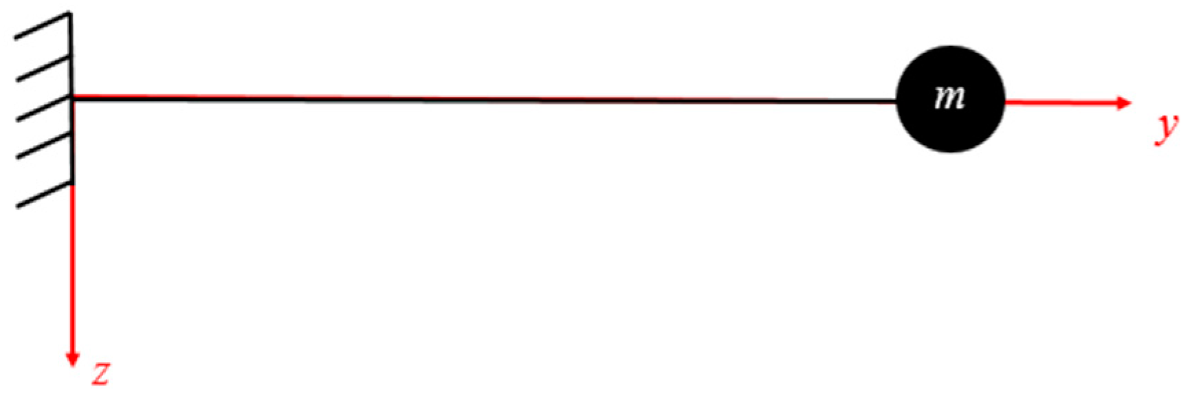
3.1. Static Analysis: Free-End Displacement

With reference to Figure 2, the free-end displacement is computed by the Virtual Work Principle (VWP). In particular, the strain field $\mathrm{S}\left(\mathrm{y},\mathrm{z}\right)$ and the displacement field $\mathrm{v}(\mathrm{z},\mathrm{y})$ along the beam axis are linked by the relation:

$$\mathrm{S}\left(\mathrm{y},\mathrm{z}\right)=\frac{\partial \mathrm{v}\left(\mathrm{z},\mathrm{y}\right)}{\partial \mathrm{y}}$$

(5)

In a generic system Π, the displacement field can be determined by minimizing the relative potential energy with the Rayleigh–Ritz method: the displacement field is therefore a linear combination of a function $\mathrm{f}(\mathrm{y},\mathrm{z})$, and its $\mathrm{m}-1$ differentials via m coefficients are calculated as follows:

$$\frac{\partial \mathsf{\Pi }}{\partial {\mathrm{c}}_{\mathrm{i}}}=0\mathrm{i}=1,\dots ,\mathrm{m}$$

(6)

In the case of the bending beam, according to the Euler–Bernoulli theory, the axial displacement field can be given as a function of the rotation ${\mathsf{\phi }}_{\mathrm{x}}$ and the orthogonal displacement field $\mathrm{w}\left(\mathrm{y}\right)$:

$$\mathrm{v}\left(\mathrm{y},\mathrm{z}\right){=\mathrm{z}\mathsf{\phi }}_{\mathrm{x}}=\mathrm{z}\frac{\partial \mathrm{w}\left(\mathrm{y}\right)}{\partial \mathrm{y}}$$

(7)

with $\mathrm{w}\left(\mathrm{y}\right)$ being a Hermite polynomial function. Since the axial strain field is obtained as the differential of the axial displacement field $\mathrm{v}\left(\mathrm{y},\mathrm{z}\right)$ with respect to $\mathrm{y}$, the z displacement field has to be a second-degree polynomial, so that the strain field is at least constant. However, when a continuous domain is discretized via finite elements that are linked through several nodes, a displacement field is valid if there is a correspondence between the total degree of freedom of the nodes and the number of $\mathrm{m}$ coefficients used. Therefore, the minimum degree possible for the sought polynomial is the third degree:

$$\mathrm{w}\left(\mathrm{y}\right){=\mathrm{c}}_0{+\mathrm{c}}_1{\mathrm{y}+\mathrm{c}}_2{\mathrm{y}}^2{+\mathrm{c}}_3{\mathrm{y}}^3$$

(8)

Given that $\mathrm{y}\in [0,\mathrm{l}]$ and the boundary conditions $\mathrm{w}\left(0\right)=0$ and $\dot{\mathrm{w}}\left(0\right)=0$ imposed by the joint configuration, it can be simply verified that the first two constants are null, so that the elastic internal energy is:

$${\mathrm{E}}_{\mathrm{el}}=\frac{1}{2}\mathrm{EI}{{\displaystyle \int }}_0^{\mathrm{l}}{\left(\frac{{\partial }^2\mathrm{w}}{\partial {\mathrm{y}}^2}\right)}^2\mathrm{dy}=\frac{1}{2}\mathrm{EI}\left[{4\mathrm{c}}_2^2{\mathrm{l}+12\mathrm{c}}_2{\mathrm{c}}_3{\mathrm{l}}^2{+12\mathrm{c}}_3^2{\mathrm{l}}^3\right]$$

(9)

Naturally, ${\mathrm{E}}_{\mathrm{el}}$ is related to the displacement of the beam free end by the relation:

$${\mathrm{E}}_{\mathrm{el}}=-\mathrm{F}\times \mathrm{w}\left(\mathrm{l}\right)=\left({\mathrm{Fc}}_2{\mathrm{l}}^2{+\mathrm{Fc}}_3{\mathrm{l}}^3\right)$$

(10)

From (9) and (10), ${\mathrm{c}}_2$ and ${\mathrm{c}}_3$ are determined. In particular:

$$\mathrm{w}\left(\mathrm{y}\right)=\frac{\mathrm{F}}{2\mathrm{EI}}\left(\frac{1}{3}{\mathrm{y}}^3-\mathrm{l}\right)$$

(11)

$$\mathrm{w}\left(\mathrm{l}\right)=-\frac{{\mathrm{Fl}}^3}{3\mathrm{EI}}$$

(12)

Once the shape function is introduced:

$${\mathrm{b}}_{\mathrm{s}}\left(\mathrm{y}\right)=\frac{\mathrm{w}\left(\mathrm{y}\right)}{\mathrm{w}\left(\mathrm{l}\right)}=\frac{3}{2}{\left(\frac{\mathrm{y}}{\mathrm{l}}\right)}^2-\frac{1}{2}{\left(\frac{\mathrm{y}}{\mathrm{l}}\right)}^3$$

(13)

the strain field can be written as:

$$\mathrm{v}\left(\mathrm{y},\mathrm{z}\right)=\mathrm{z}\frac{\partial \mathrm{w}\left(\mathrm{y}\right)}{\partial \mathrm{y}}\to {\mathrm{S}}_{\mathrm{y}}=\frac{\partial \mathrm{v}\left(\mathrm{y},\mathrm{z}\right)}{\partial \mathrm{y}}=\frac{\mathrm{z}{\partial }^2\mathrm{w}\left(\mathrm{y}\right)}{\partial \mathrm{y}}=\mathrm{z}\left[\frac{3}{{\mathrm{l}}^2}-\frac{3\mathrm{y}}{{\mathrm{l}}^3}\right]\mathrm{w}\left(\mathrm{l}\right)=\mathrm{g}\left(\mathrm{z},\mathrm{y}\right)\mathrm{w}\left(\mathrm{l}\right)$$

(14)

Concerning the (12), which refers to a homogeneous beam, an equivalent expression can be given for a composite beam, using an approximated calculation of the stiffness [27]:

$$\mathrm{K}=\frac{\mathrm{F}}{\mathrm{w}}=\frac{3\mathrm{D}}{{\mathrm{l}}^3}$$

(15)

The modeled beam is a composite, so that (15) represents an approximation with respect to the Classical Lamination Theory. The comparison between the results obtained by the analytical model and the finite element (FE) model will give a measure of this approximation. The parameter D is the equivalent to the Young constant of a homogenous beam multiplied by its bending inertial moment, so that for a composite beam, it results in the following:

$${\mathrm{D}=\mathrm{E}}_{\mathrm{i}}{\times \mathrm{I}}_{\mathrm{i}}$$

(16)

The inertial moment of the generic layer is related to its thickness, its width, and the orthogonal distance between its center of mass and the neutral bending axis. The neutral bending axis position can be found according to the geometric/mechanical properties of the layers considered. Assuming the lower layer as the steel one, the neutral bending axis coordinate is:

$${\mathrm{z}}_{\mathrm{n}}=1.02\mathrm{mm}$$

(17)

Consequently, it results in the following:

$$\begin{gathered} {\mathrm{I}}_{\mathrm{STE}}=3.87{\mathrm{mm}}^4 \\ {\mathrm{I}}_{\mathrm{PZT}}=6.76{\mathrm{mm}}^4 \end{gathered}$$

(18)

$$\mathrm{D}=1.35{\mathrm{Nm}}^2$$

(19)

$${\mathrm{K}}_{\mathrm{mech}}=94.5\mathrm{kN}/\mathrm{m}$$

(20)

$$\mathrm{w}\left(\mathrm{l}\right)=\frac{\mathrm{F}}{{\mathrm{K}}_{\mathrm{mech}}}=\frac{54.88}{94500}=0.58\mathrm{mm}$$

(21)

An equivalent stiffness of the PZT material can be determined by using the constitutive piezoelectric Equation (1). Since:

$${\mathrm{V}}_{\mathrm{A}}-{\mathrm{V}}_{\mathrm{B}}=-{{\displaystyle \int }}_{\mathrm{A}}^{\mathrm{B}}\overrightarrow{\mathrm{E}}\mathrm{x}\overrightarrow{\mathrm{dl}}$$

(22)

by assuming a mono-dimensional and constant electric field, and by imposing ${\mathrm{V}}_{\mathrm{A}}=0$, the voltage ${\mathrm{V}}_{\mathrm{B}}$ is obtained:

$${\mathrm{V}}_{\mathrm{B}}=-\mathrm{E}\times \mathrm{z}\to \mathrm{E}=-\frac{{\mathrm{V}}_{\mathrm{B}}}{\mathrm{z}}{=\mathrm{b}}_{\mathrm{e}}{\left(\mathrm{z}\right)\times \mathrm{q}}_{\mathrm{e}}$$

(23)

The electric stiffness of the system can be calculated by imposing that the internal work ${\mathrm{L}}_{\mathrm{int}}$ is the result of the work where the stresses perform for the virtual strains $\mathsf{\delta }\mathrm{S}$, and the one that the electric displacement performs for the virtual electric field $\mathsf{\delta }\mathrm{E}$. Thus, by expressing the stress and the electric displacement according to Equation (1), the following relation can be written:

$${\mathrm{L}}_{\mathrm{int}}={{\displaystyle \int }}_{\mathrm{V}}^{}{\mathrm{S}}^{\mathrm{T}}{\mathrm{c}}^{\mathrm{T}}\mathsf{\delta }\mathrm{S}\mathrm{dV}-{{\displaystyle \int }}_{\mathrm{V}}^{}{\mathrm{E}}^{\mathrm{T}}{\mathrm{e}}^{\mathrm{T}}\mathsf{\delta }\mathrm{S}\mathrm{dV}+{{\displaystyle \int }}_{\mathrm{V}}^{}{\mathrm{S}}^{\mathrm{T}}{\mathrm{e}}^{\mathrm{T}}\mathsf{\delta }\mathrm{E}\mathrm{dV}+{{\displaystyle \int }}_{\mathrm{V}}^{}{\mathrm{E}}^{\mathrm{T}}{\mathsf{\epsilon }}^{\mathrm{T}}\mathsf{\delta }\mathrm{E}\mathrm{dV}$$

(24)

Using (14) and (23), the integrals in (24) can be evaluated by assuming a linear behavior, and by splitting each contribution in the correspondent layer. In particular, the steel layer will contribute only to the stiffness term, while the PZT one will contribute to all terms. Given the isotropic assumption for the PZT and that the Young modules are constants, the mechanical stiffness is calculated as:

$${\mathrm{K}}_{\mathrm{mech}}={\displaystyle \sum }_{\mathrm{i}=1}^2{\mathrm{E}}_{\mathrm{i}}{{\displaystyle \int }}_{\mathrm{A}}^{}{\mathrm{z}}^2\mathrm{dA}{{\displaystyle \int }}_0^{\mathrm{l}}{\overline{\mathrm{g}}}^2\mathrm{dy}$$

(25)

where the term $\overline{\mathrm{g}}\left(\mathrm{y}\right)=\mathrm{g}(\mathrm{z},\mathrm{y})/\mathrm{z}$ is defined in order to separate the surface and the linear integrals.

The surface integral of ${\mathrm{z}}^2$ is the inertial moment with respect to the x-axis, and it has already been calculated in (18). By computing the remaining integral, the mechanical stiffness of the beam is derived:

$${\mathrm{K}}_{\mathrm{mech}}=\frac{3}{{\mathrm{l}}^3}\left({\mathrm{E}}_{\mathrm{PZT}}{\times \mathrm{I}}_{\mathrm{xPZT}}{+\mathrm{E}}_{\mathrm{STE}}{\times \mathrm{I}}_{\mathrm{xSTE}}\right)=\frac{3\mathrm{D}}{{\mathrm{l}}^3}=94.5\mathrm{kN}/\mathrm{m}$$

(26)

which obviously coincides with (20), since this term is not affected by the electro-mechanical effect.

The volume piezoelectric coupling constant is given by:

$$\mathsf{\Theta }=-{{\displaystyle \int }}_{\mathrm{V}}^{}{\mathrm{g}}_{\mathrm{s}}\left(\mathrm{z},\mathrm{y}\right){\mathrm{e}}_{\mathrm{i}}^{}{\mathrm{b}}_{\mathrm{e}}\left(\mathrm{z}\right)\mathrm{dV}$$

(27)

Based on the computed strain along y and electric field along z, by taking into account the piezoelectric constant ${\mathrm{e}}_{32}=-10.1\mathrm{NV}/\mathrm{m}$, (27) becomes:

$${\mathsf{\Theta }=-\mathrm{e}}_{32}{{\displaystyle \int }}_{\mathrm{V}}^{}\mathrm{z}\left(\frac{3}{{\mathrm{l}}^2}-\frac{3\mathrm{y}}{{\mathrm{l}}^3}\right)\ast \frac{1}{\mathrm{z}}{\mathrm{dV}=-\mathrm{e}}_{23}{\mathrm{s}}_{\mathrm{PZT}}\mathrm{b}{{\displaystyle \int }}_0^{\mathrm{l}}\left(\frac{3}{{\mathrm{l}}^2}-\frac{3\mathrm{y}}{{\mathrm{l}}^3}\right)\mathrm{dy}=2.4\mathrm{mN}/\mathrm{V}$$

(28)

Hence, the PZT volume dielectric constant is calculated as:

$${\mathrm{C}}_{\mathrm{p}}={{\displaystyle \int }}_{\mathrm{V}}^{}{\mathrm{b}}_{\mathrm{e}}^{}\left(\mathrm{z}\right){\mathsf{\epsilon }}_{\mathrm{i}}{\mathrm{b}}_{\mathrm{e}}\left(\mathrm{z}\right)\mathrm{dV}$$

(29)

The polarization occurs along z, and it is assumed to be independent of the length and the width of the beam. The remaining integral can be therefore computed as:

$${\mathrm{C}}_{\mathrm{p}}=\frac{{\mathsf{\epsilon }}_3\mathrm{lb}}{{\mathrm{s}}_{\mathrm{PZT}}}=6.73\mathrm{n}F$$

(30)

Analogously, the external work is based on the contributions of the work surface charge density ${\mathsf{\sigma }}_{\mathrm{e}}$, and the external force $\mathrm{F}$:

$${\mathrm{L}}_{\mathrm{ext}}={{\displaystyle \int }}_{\mathrm{A}}{\mathsf{\sigma }}_{\mathrm{e}}\mathsf{\delta }{\mathrm{V}}_{\mathrm{B}}\mathrm{dA}+{\mathrm{F}}^{\mathrm{T}}\mathsf{\delta }\mathrm{w}\left(\mathrm{l}\right)$$

(31)

By constraining ${\mathrm{L}}_{\mathrm{ext}}$ to zero, the integral constitutive equation for the beam is derived:

$$\{\begin{array}{c}{\mathrm{K}}_{\mathrm{mecc}}\mathrm{W}-\mathsf{\Theta }\mathrm{V}=\mathrm{F}\\ {\mathrm{C}}_{\mathrm{p}}\mathrm{V}+\mathsf{\Theta }\mathrm{W}=0\end{array}$$

(32)

from which the electric equivalent stiffness of the beam is obtained as:

$${\mathrm{K}}_{\mathrm{elmec}}{=\mathrm{K}}_{\mathrm{mecc}}\left(1+\frac{{\mathsf{\Theta }}^2}{{\mathrm{C}}_{\mathrm{p}}{\mathrm{K}}_{\mathrm{mecc}}}\right)=95400\mathrm{N}/\mathrm{m}$$

(33)

Equation (33) is higher than the (20). Indeed, the electric properties of PZT tighten up the system and, consequently, the actual displacement of the free end is lower than (21):

$$\mathrm{w}\left(\mathrm{l}\right)=\frac{\mathrm{F}}{{\mathrm{K}}_{\mathrm{elmecc}}}=0.58\mathrm{mm}$$

(34)

The deformed shapes of the beam have been represented in Figure 3, solving the displacement field in a Matlab^® script.

After the analytical solution, a 3D model of the support has been produced with Ansys^® Mechanical APDL, to determine both the mechanical and the electric–mechanical responses, in terms of the free-end displacement of the beam. SHELL281 elements have been used in purely mechanical analyses, with these being the most suitable for the analysis of a thin composite structure. The deformed shapes for the isotropic and the orthotropic models are depicted, respectively, in Figure 4.

Comparing the analytical results (21) with the simulation ones in 4a and 4b, and (34) with 4c and 4b, the deviations in

Table 5. Deviations.

Deviation	Mechanical	Piezoelectric
Model	$1.26\%$	$-0.14\%$
Isotropic approximation	$0.15\%$	$-1.53\%$

have been found:

With reference to the first column of the table, it is evident that in an isotropic condition, the FE model is stiffer than the analytical one. This aspect can be attributed to the discretization operated by the meshing process. Naturally, the orthotropic model registers a higher deviation, even though the accuracy is still acceptable. A purely mechanical analysis has been performed with the SOLID226 model, whose results are consistent with analytical ones.

All of the results from the analytical analyses are summarized in

Table 6. Static analysis results.

$\left[\mathbf{mm}\right].$	Analytical Model	SHELL281 Model		SOLID226 Model
	Isotropic	Isotropic	Orthotropic	Isotropic	Orthotropic
${\mathbf{w}}_{\mathbf{mec}}$	$0.58$	$0.57$	$0.58$	$0.58$	$0.58$
${\mathbf{w}}_{\mathbf{el}}$	$0.58$			$0.58$	$0.58$
${\mathbf{K}}_{\mathbf{mec}}$	$94512$	$95710$	$94360$	$95234$	$93901$
${\mathbf{K}}_{\mathbf{el}}$	$95385$			$95250$	$93935$
${\mathbf{D}}_{\mathbf{el}}$	$1.36$			$1.36$	$1.34$
${\mathbf{E}}_{\mathbf{el}}$	$7.58{\times 10}^{10}$			$7.55{\times 10}^{10}$	$7.27{\times 10}^{10}$

.

It should be pointed out that the Young constant derived from the piezoelectric results of the SOLID226 model gives ${\mathrm{E}}_{\mathrm{PZT}}=72.7\mathrm{GPa}$.

3.2. Static Analysis: Buckling

When a structure has a preponderant dimension with respect to the other two, an instability may occurs if the mechanical stress acts along the considered direction. To analysis this aspect in the case of an embedded beam with an axial force exerted on the free end, the beam equilibrium is considered with respect to the deformed shape, since the hypothesis of small displacements no longer applies.

The critical buckling load for a composite beam can be evaluated by the Euler relation (16):

$${\mathrm{P}}_{\mathrm{cr}}=\frac{1}{4}\frac{{\mathsf{\pi }}^2\mathrm{D}}{{\mathrm{l}}^2}=2704\mathrm{N}$$

(35)

where $\mathrm{l}$ is the beam length and $\mathrm{C}$ is a constrain factor. The evaluated critical load is two orders of magnitude bigger than the load considered in this context, $\mathrm{F}=54.88\mathrm{N}$, so that the stability test is satisfied. By considering the slim ratio $\mathrm{l}/\mathrm{k}$, the buckling analysis also has to be extended to the Euler buckling hyperbole, which is defined by the relation:

$${\mathrm{T}}_{\mathrm{cr}}=\frac{{\mathrm{P}}_{\mathrm{cr}}}{\mathrm{A}}=\frac{1}{4}\frac{{\mathsf{\pi }}^2\mathrm{E}}{{\left(\frac{\mathrm{l}}{\mathrm{k}}\right)}^2}$$

(36)

Finally, the Johnsons critical stress also has to be considered:

$${\mathrm{T}}_{\mathrm{cr}}{=\mathrm{T}}_{\mathrm{y}}-{\left(\frac{{\mathrm{T}}_{\mathrm{y}}}{2\mathsf{\pi }}\right)}^2\frac{4}{\mathrm{E}}{\left(\frac{\mathrm{l}}{\mathrm{k}}\right)}^2$$

(37)

The intersection between (36) and the (37), represented in Figure 5a, gives the threshold slim ratio, such that if the slim ratio of the considered beam is smaller than this limit, the critical stress has to be calculated with (36), otherwise (37) must be used. In this case, the threshold slim ratio is higher than the beam slim ratio, so that the critical load is evaluated via (37):

$${\mathrm{P}}_{\mathrm{cr}}=573\mathrm{N}$$

(38)

From (38), it can be deduced that the bucking verification is also satisfied.

The same analysis has been performed on the SHELL281 model, and the eigenvalues in Figure 5b have been obtained. The buckling analysis can indeed be expressed as an eigenvalues problem resulting from the deformed shape equilibrium:

$$(\mathrm{K}+\mathsf{\lambda }{\mathrm{K}}_{\mathrm{G}})\mathrm{v}=\mathsf{\lambda }{\mathrm{P}}^{\ast }$$

(39)

where $\mathrm{K}$ is the stiffness matrix of the system, ${\mathrm{K}}_{\mathrm{G}}$ is the geometric stiffness matrix of the system, whose value depends on the baseline load fixed ${\mathrm{P}}^{\ast }$, and $\mathsf{\lambda }$ is an eigenvalue such that the characteristic polynomial $\left|\mathrm{K}+\mathsf{\lambda }{\mathrm{K}}_{\mathrm{G}}\right|=0$.

Supposing a baseline load ${\mathrm{P}}^{\ast }$, a static analysis followed by the buckling analysis has been performed, obtaining the eigenvalues in Figure 5b. It has to be noted that since the beam is a composite, the instability could be misinterpreted as an excessive bending reaction. With respect to the first positive eigenvalue, the Euler critical load can be determined as:

$${\mathrm{P}}_{\mathrm{cr},\mathrm{mod}}=49.8\mathrm{P}\mathrm{b}=2733\mathrm{N}$$

(40)

so that the deviation between the analytical model (35) and the FE model (40) can be calculated as:

$$\mathsf{\epsilon }=\frac{2704-2733}{2704}=-1.08\%$$

(41)

The software has therefore overestimated the structural resistance, although the deviation is acceptable.

3.3. Dynamic Analysis: Fatigue

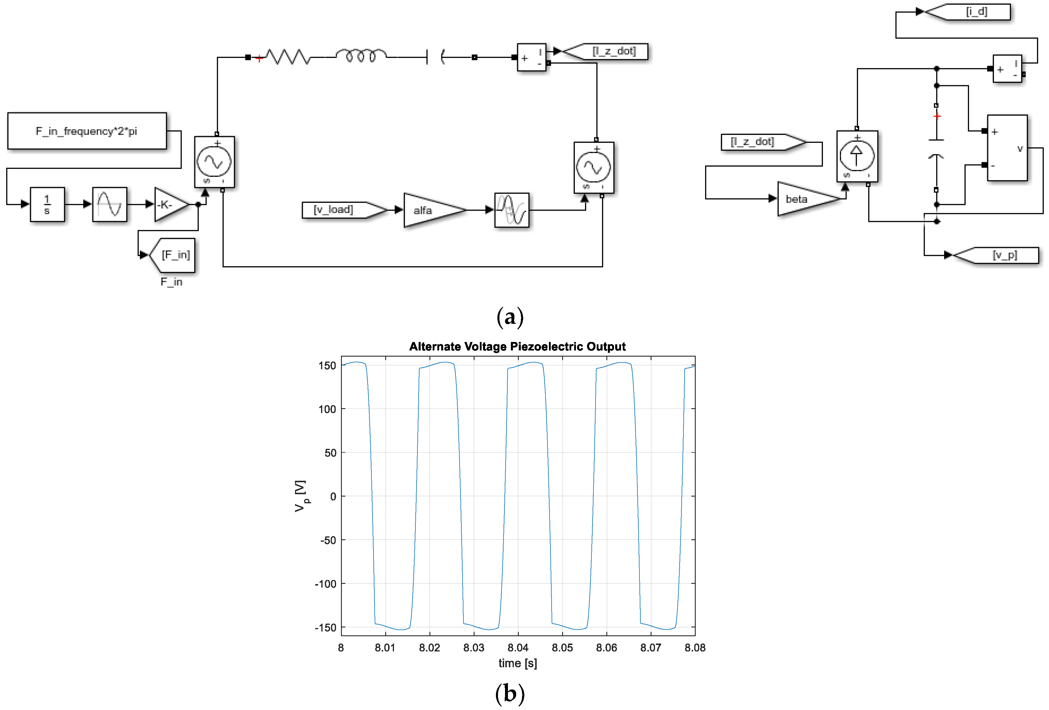
The mechanical stress applied on the free end of the support is an alternative bending with amplitude:

$${\mathrm{T}}_{\mathrm{a}}=\frac{{\mathrm{T}}_{\max }{-\mathrm{T}}_{\min }}{2}=0.24{10}^8\mathrm{GPa}$$

(42)

The frequency of the load is equal to the speed of the rotor, set to $3000\mathrm{rpm}$, $4500\mathrm{rpm}$, and $6000\mathrm{rpm}$. The amplitude is maintained as a constant for the variation of the speed, by adjusting the eccentricity value. In this case, the term eccentricity has been improperly used to represent the product between the mass and the actual eccentricity, i.e., the distance between the center of mass and the center of rotation. The three load curves have been plotted in Figure 6a with respect to the period of the slower one, while the Whӧler plot of the material has been represented in Figure 6b. This plot is divided in three successive parts: the first part, low fatigue cycle (LFC), starts from the ultimate strength of the material, and the third part is a plateau representing the stress magnitude that corresponds to an infinite life of the component (Cutoff), while for the second part high fatigue cycle (HFC) the following relation has been used:

$${\ln \mathrm{S}}_{\mathrm{f}}=\ln \mathrm{a}+\mathrm{b}\ln \mathrm{N}$$

(43)

where $\mathrm{a}$ and $\mathrm{b}$ are two parameters derived by forcing the line (43) to pass through the following points:

$$\begin{gathered} \mathrm{A}\left({10}^3{,\mathrm{S}}_{\mathrm{f}}\left({10}^3\right)\right) \\ {\mathrm{B}(10}^6{,\mathrm{S}}_{\mathrm{e}}) \end{gathered}$$

(44)

with ${\mathrm{S}}_{{\mathrm{f}(10}^3)}$ as the maximum stress amplitude that can be applied for ${10}^3$ cycles before collapse, and ${\mathrm{S}}_{\mathrm{e}}$ as the cutoff stress limit. While ${\mathrm{S}}_{\mathrm{f}({10}^3)}$ can be estimated from the ultimate strength via a factor $\mathrm{f}<1$, which decreases as the ultimate strength increases, ${\mathrm{S}}_{\mathrm{e}}$ can be assigned once the stress amplitude ${\mathrm{S}}_{\mathrm{e}}^{\prime }$ is identified. Once ${\mathrm{S}}_{\mathrm{e}}^{\prime }$, the fatigue limit of a sample that is stressed with alternative bending, is estimated as being half the ultimate strength of the material, ${\mathrm{S}}_{\mathrm{e}}$ is obtained as:

$${\mathrm{S}}_{\mathrm{e}}{=\mathrm{k}}_{\mathrm{a}}{\mathrm{k}}_{\mathrm{b}}{\mathrm{k}}_{\mathrm{c}}{\mathrm{k}}_{\mathrm{d}}{\mathrm{k}}_{\mathrm{e}}{\mathrm{S}}_{\mathrm{e}}^{\prime }=241\mathrm{MPa}$$

(45)

The Whӧler plot parameters and the service life of the component can then be evaluated:

$$\mathrm{N}={\left[\frac{{\mathrm{T}}_{\mathrm{a}}}{\mathrm{a}}\right]}^{\frac{1}{\mathrm{b}}}=1.04{\times 10}^6\mathrm{cycles}$$

(46)

Inter alia, in this case, since the cutoff limit (45) is above the stress amplitude exerted on the material (42), the service life of the component has been assumed as being infinite.

3.4. Dynamic Analysis: Equation of Motion

The rotor-support system can be modeled according to the Jeffcott rotor model, assuming a rigid rotor suspended on elastic supports. The rotor is assumed to be fixed at the mid-section of the drive, so that the system is symmetrical with respect to the yz plane. The four supports, assumed to be identical, have been modeled as a spring-damper system with uniform stiffness and dumping coefficients in the y and z directions. If the rotor is statically unbalanced, the motion equations can be written as [28]:

$$\{\begin{array}{c}\mathrm{m}\ddot{\mathrm{z}}{+\mathrm{c}\dot{\mathrm{z}}+\mathrm{kz}=\mathrm{me}\mathsf{\omega }}^2\cos \left(\mathsf{\omega }\mathrm{t}\right)\\ \mathrm{m}\ddot{\mathrm{y}}{+\mathrm{c}\dot{\mathrm{y}}+\mathrm{ky}=\mathrm{me}\mathsf{\omega }}^2\sin \left(\mathsf{\omega }\mathrm{t}\right)\end{array},$$

(47)

with $\mathrm{m}$ as the rotor mass and $\mathrm{e}$ as the eccentricity. Given the aforementioned assumptions, the motions along the two axis are therefore decoupled. In particular, the force amplitude evaluated in (4) is exerted on each support, so that the following relation applies:

$${2\mathrm{F}=\mathrm{me}\mathsf{\omega }}^2,$$

(48)

Given that (48) is constant, the three resulting eccentricity values are immediately obtained; they are listed in

Table 7. Static analysis results.

$\mathbf{Speed}\left[\mathbf{rpm}\right]$	$3000$	$4500$	$6000$
Speed $\left[\frac{\mathrm{rad}}{\mathrm{s}}\right]$	$314$	$471$	$628$
Frequency $\left[\mathrm{Hz}\right]$	$50$	$75$	$100$
m e $\left[\mathrm{kg}\mathrm{m}\right]$	$1.11{\times 10}^{-3}$	$4.94{\times 10}^{-4}$	$2.78{\times 10}^{-4}$

.

Clearly, the eccentricity decreases with progressively smaller decrements as the speed increases.

By considering a rotor with a length of $80\mathrm{mm}$ and a diameter $50\mathrm{mm}$, a balanced mass, ${\mathrm{m}}_1=1.78\mathrm{kg}$, is derived. The eccentricity property is then conferred to the system by removing $\mathrm{n}$ identical masses with a constant phase shift of $15°$, starting from the mass ${\mathrm{m}}_{\mathrm{n}}$ at $\mathsf{\theta }=0°$. Since the masses are symmetrically positioned with respect to the y-axis, the resultant mass center is simply shifted along the y-axis. By putting $\mathrm{n}=13,$ and by solving the corresponding system of equations, the values listed in

Table 8. Mass and eccentricity values for each rotor speed.

$\mathbf{Values}$	$1.11{\times 10}^{-3}$	$4.94{\times 10}^{-4}$	$2.78{\times 10}^{-4}$
Unbalancing masses [kg]	$5.23{\times 10}^{-3}$	$2.23{\times 10}^{-3}$	$1.31{\times 10}^{-3}$
Eccentricity [m]	$6.50{\times 10}^{-4}$	$2.28{\times 10}^{-4}$	$1.58{\times 10}^{-4}$
Holes radius [m]	$1.60{\times 10}^{-3}$	$1.08{\times 10}^{-3}$	$0.81{\times 10}^{-3}$
Rotor mass [kg]	$1.71$	$1.75$	$1.76$

are calculated:

The rotor masses included in Table 8 correspond to twice the mass of the rotor supports, which, indeed, has been schematized as pinned–pinned beams stressed by a concentrated force applied at the mid-section. This approximation leads to an underestimation of the resonance frequencies of the system.

With respect to the system stiffness, each support contributes to the values of the analytic electric stiffness and the SOLID226 electric stiffness found in Table 6.

$${\mathrm{K}}_{\mathrm{el},\mathrm{an}}=95385\mathrm{N}/\mathrm{m}$$

$${\mathrm{K}}_{\mathrm{el},\mathrm{SOL}}=93935\mathrm{N}/\mathrm{m}$$

Assuming the stiffness constant with the speed, both the resonance frequencies and the critical dumping coefficients can be evaluated according to the following relations (see also

Table 9. Mass and eccentricity values for each rotor speed.

$\mathbf{M}\left[\mathbf{kg}\right].$	$0.85$		$0.90$		$0.91$
$\mathrm{Model}$	$1\mathrm{D}$	$\mathrm{SOLID}$	$1\mathrm{D}$	$\mathrm{SOLID}$	$1\mathrm{D}$	$\mathrm{SOLID}$
${\mathrm{f}}_{\mathrm{M}}\left[\mathrm{Hz}\right]$	$53.16$	$52.75$	$52.58$	$52.18$	$52.39$	$51.99$
${\mathsf{\omega }}_{\mathrm{n}}[\mathrm{rad}/\mathrm{s}]$	$334.02$	$331.47$	$330.39$	$327.87$	$329.15$	$326.64$
$\mathrm{n}\left[\mathrm{rpm}\right]$	$3189.62$	$3165.29$	$3154.96$	$3130.91$	$3143.10$	$3119.14$
${\mathrm{C}}_{\mathrm{CR}}$	$571.14$	$566.78$	$577.41$	$573.01$	$579.59$	$575.17$

):

$$\begin{gathered} {\mathsf{\omega }}_{\mathrm{n}}=\sqrt{\mathrm{K}/\mathrm{M}} \\ {\mathrm{C}}_{\mathrm{CR}}=2\sqrt{\mathrm{KM}} \end{gathered}$$

(49)

As expected, as the mass increases at a constant stiffness, and the natural frequency decreases.

The damping action of the system represents the hysteretic/friction phenomena that occur within and between the system parts. To calculate the corresponding coefficients, various methods can be used, and generally, the experimental interpolation of the data collected from the actual system methods are preferred. In this case, however, the proportional analytical damping model has been adopted:

$$\mathrm{C}=\mathsf{\alpha }\mathrm{M}+\mathsf{\beta }\mathrm{K}$$

(50)

Once the coefficients are assumed to be equal, the corresponding value can be calculated by fixing the magnitude of the damping ratio $\mathsf{\xi }$. Inter alia, if $\mathsf{\xi }<1$ is fixed, the system law of motion will be an actual vibration, otherwise it would return with an exponential behavior to its initial condition. This assumes that the system has not been irreparably perturbed, in which case, it can either reach a new equilibrium state, or remain in a non-equilibrium state that can eventually take it to collapse. The values of the damping coefficients are reported in

Table 10. Damping coefficients and damping rotations for the three speeds considered for the analytical model and the FE model.

M [kg]	0.85		0.90		0.91
Model	1D	SOLID	1D	SOLID	1D	SOLID
C [Ns/m]	399.80	393.72	399.80	393.72	399.80	393.72
ξ	0.70	0.69	0.69	0.69	0.69	0.68

for different system configurations.

From the parameter characterization, it is finally possible to determine the motion law. By focusing on an upper support (the same results can be extended to a lower support), the dynamic Equation (47) can be written as:

$$\ddot{\mathrm{w}}+2\mathsf{\xi }{\mathsf{\omega }}_{\mathrm{n}}\dot{\mathrm{w}}+{\mathsf{\omega }}_{\mathrm{n}}^2\mathrm{w}=-\frac{\mathrm{F}}{\mathrm{M}}\sin \mathsf{\omega }\mathrm{t}$$

(51)

from which:

$$\mathrm{w}\left(\mathrm{t}\right)=-\frac{\mathrm{F}}{\mathrm{K}}\mathsf{\chi }\left(\mathsf{\beta }\right)\sin \left(\mathsf{\omega }\mathrm{t}-\mathsf{\psi }\left(\mathsf{\beta }\right)\right)$$

(52)

The value of the gain factor $\mathsf{\chi }$, of the speed ratio $\mathsf{\beta }=\frac{\mathsf{\omega }}{{\mathsf{\omega }}_{\mathrm{n}}}$ and of the phase angle $\mathsf{\psi }$ are reported in

Table 11. Amplification factors and phase angles of the law of motions for the three considered speeds.

M [kg]	0.85		0.90		0.91
${\mathsf{\omega }}_{\mathrm{F}}$ [rad/s]	314		471		628
Model	1D	SOLID	1D	SOLID	1D	SOLID
β	0.94	0.95	1.43	1.43	1.91	1.92
χ	0.76	0.76	0.45	0.45	0.27	0.27
ψ [rad]	1.48	1.49	–1.09	–1.08	–0.78	–0.77

for different speed values.

As expected, the gain factor is maximum when the rotor speed equals $3000\mathrm{rpm}$, as the resonance frequency of the system is at $3190\mathrm{rpm}$. It should be noted that the piezoelectric materials guarantee the best electro-mechanical conversion at around their resonance frequency, where indeed, the impedance of the correspondent equivalent electrical flow is minimized. The time behavior of motion, speed and acceleration at the three considered speeds is plotted in Figure 7.

The dynamic analyses have been performed on the SHELL281 FE model by including a MASS21 element whose $\mathrm{R}\mathrm{C}\mathrm{s}$ has been derived from the mass values shown in Table 9. With respect to the values listed in Table 8, the following deviations regarding the natural frequencies have been calculated:

$${\mathsf{\epsilon }}_{\mathrm{M}1}=\frac{53.15-52.75}{53.15}=0.75\%$$

$${\mathsf{\epsilon }}_{\mathrm{M}2}=\frac{51.89-51.49}{51.89}=0.77\%$$

$${\mathsf{\epsilon }}_{\mathrm{M}3}=\frac{51.46-51.07}{51.46}=0.76\%$$

It should be pointed out that all the estimated errors are very small.

4. Electric Analysis

The charge Q that accumulates on the PZT surfaces as an effect of the applied mechanical stress can be collected by connecting a load, such as a resistor ${\mathrm{R}}_{\mathrm{L}}$, via two electrodes anchored on the PZT surfaces. The current in the PZT-R_L circuit can naturally be expressed as:

$${\mathrm{I}}_{\mathrm{L}}=\frac{\mathrm{dQ}}{\mathrm{dt}}=+\frac{\mathrm{V}}{{\mathrm{R}}_{\mathrm{L}}}$$

(53)

By discretizing (53) with respect to a sample time interval ∆t, the following relation is obtained:

$${\mathrm{Q}}_{\mathrm{n}+1}{=\mathrm{Q}}_{\mathrm{n}}-\mathrm{V}\frac{\Delta \mathrm{t}}{{\mathrm{R}}_{\mathrm{L}}}$$

(54)

Equation (54) can be solved once the initial value ${\mathrm{Q}}_0$ is determined. Naturally, the evaluation of the ${\mathrm{Q}}_{\mathrm{n}+1}$ is an iterative process, whose number of iterations depends on the ratio $\Delta \mathrm{t}$/${\mathrm{R}}_{\mathrm{L}}$. The voltage V can be computed, starting from the expression of the electric displacement flux density through the piezoelectric material:

$${\mathrm{D}}_{\mathrm{i}}{=-\mathrm{q}}_{\mathrm{c}}$$

(55)

with ${\mathrm{q}}_{\mathrm{c}}$ as the surface charge. The electric displacement can be also expressed as a combination of the strain and the electric field according to the constitutive Equation (1), where, since only the component of the strain along the support axis applies, can be characterized by the piezoelectric coefficient ${\mathrm{e}}_{3,2}$:

$${\mathrm{e}}_{3,2}{\times \mathrm{S}}_{\mathrm{y}}{(\mathrm{y},\mathrm{z})-\mathsf{\epsilon }}^{\mathrm{S}}\frac{\partial \mathrm{V}}{\partial \mathrm{z}}{=\mathrm{q}}_{\mathrm{c}}$$

(56)

By imposing ${\mathrm{Q}}_0=0$, by taking into account (14), and by expressing the free-end displacement according to (52), (56) leads to:

$$\mathrm{V}\left(\mathrm{y},\Delta {\mathrm{t},\mathrm{R}}_{\mathrm{L}}\right)=\frac{\frac{{\mathrm{e}}_{2,3}}{{\mathsf{\epsilon }}^{\mathrm{S}}}\left[\frac{{\mathrm{s}}_{\mathrm{PZT}}^2}{2}\left(\frac{3}{{\mathrm{l}}^2}-\frac{3\mathrm{y}}{{\mathrm{l}}^3}\right)\left(-\frac{\mathrm{F}}{\mathrm{K}}\mathsf{\chi }\left(\mathsf{\beta }\right)\mathrm{sen}\left(\mathsf{\omega }\mathrm{t}-\mathsf{\psi }\left(\mathsf{\beta }\right)\right)\right)\right]}{1+\frac{\Delta \mathrm{t}}{{\mathrm{R}}_{\mathrm{L}}}{\mathrm{s}}_{\mathrm{PZT}}}$$

(57)

The voltage on the upper surface of the PZT layer is therefore linear along the length of the beam, being maximum at $\mathrm{y}=0$, where the strain also is maximum. From (57), it can be deduced that when $\Delta {\mathrm{t}/\mathrm{R}}_{\mathrm{L}}\le 10$, the voltage value is not affected by variations in $\Delta \mathrm{t}$ or ${\mathrm{R}}_{\mathrm{L}}$, while when $\Delta {\mathrm{t}/\mathrm{R}}_{\mathrm{L}}>10$, as the resistance value increases, so does do voltage values up to $\Delta {\mathrm{t}/\mathrm{R}}_{\mathrm{L}}\ge {10}^4$, at which point the voltage switches its sign and the solution becomes divergent. The aforementioned considerations are endorsed by Figure 8a,b, where the voltage is plotted in correspondence with $\mathrm{y}=\mathrm{l}/2$. The voltage behavior along the support axis is depicted instead in Figure 8c.

4.1. Equivalent Electric Circuit of PZT

From an electrical point of view, the mechanical behavior of a piezoelectric material can be modeled as an RLC series circuit [32,33]:

$${\mathrm{L}}_{\mathrm{M}}\frac{\partial {\mathrm{i}}^2}{\partial \mathrm{t}}{+\mathrm{R}}_{\mathrm{M}}\frac{\partial \mathrm{i}}{\partial \mathrm{t}}+\frac{1}{{\mathrm{C}}_{\mathrm{M}}}\mathrm{i}=\frac{\partial \mathrm{V}}{\partial \mathrm{t}}$$

(58)

where inductance ${\mathbf{L}}_{\mathbf{M}}$ is half the rotor mass of the rotor, and resistance ${\mathbf{R}}_{\mathbf{M}}$ relates to the damping mechanical coefficient, while the electric stiffness corresponds to the inverse of the capacitance ${\mathbf{C}}_{\mathbf{M}}$.

Analogously, the piezoelectric behavior can be simply modeled by a capacitor ${\mathrm{C}}_{\mathrm{P}}$ series connected to a current generator that is controlled by the output of the aforementioned equivalent electric circuit. ${\mathrm{C}}_{\mathrm{P}}$ can be calculated as:

$${\mathrm{C}}_{\mathrm{P}}=\frac{{\mathsf{\epsilon }}_3^{\mathrm{T}}\mathrm{bl}}{{2\mathrm{s}}_{\mathrm{PZT}}}=3.4\mathrm{nF}$$

(59)

The overall circuit is shown in Figure 9a, while all of the parameters are listed in

Table 12. Equivalent electric circuit parameters.

${\mathbf{n}}_{\mathbf{ROT}}.$	$\left[\mathbf{rpm}\right]$	$3000$	$4500$	$6000$
${\mathrm{L}}_{\mathrm{M}}$	$\left[\mathrm{kg}\right]$	$0.86$	$0.90$	$0.91$
${\mathrm{C}}_{\mathrm{M}}$	$\left[\raisebox{1ex}{$\mathrm{N}$}\!\left/ \!\raisebox{-1ex}{$\mathrm{m}$}\right.\right]$	$1.06{\times 10}^{-5}$	$1.06{\times 10}^{-5}$	$1.06{\times 10}^{-5}$
${\mathrm{R}}_{\mathrm{M}}$	$\left[\raisebox{1ex}{$\mathrm{Ns}$}\!\left/ \!\raisebox{-1ex}{$\mathrm{m}$}\right.\right]$	$0.70$	$0.68$	$0.68$
${\mathrm{C}}_{\mathrm{p}}$	$\left[\mathrm{nF}\right]$	$3.36$	$3.36$	$3.36$
${\mathrm{f}}_{\mathrm{M}}$	$\left[\mathrm{Hz}\right]$	$52.75$	$51.49$	$51.07$
${\mathrm{f}}_0$	$\left[\mathrm{Hz}\right]$	$55$	$55$	$55$
$\mathsf{\alpha }\mathsf{\beta }$	$\left[\frac{\mathrm{N}}{\mathrm{V}}\times \frac{\mathrm{As}}{\mathrm{m}}\right]$	$2.75{\times 10}^{-5}$	$4.45{\times 10}^{-5}$	$5.05{\times 10}^{-5}$
$\mathsf{\alpha }$	$\left[\frac{\mathrm{N}}{\mathrm{V}}\right]$	$3.71{\times 10}^{-2}$	$4.72{\times 10}^{-2}$	$5.02{\times 10}^{-2}$
$\mathsf{\beta }$	$\left[\frac{\mathrm{As}}{\mathrm{m}}\right]$	${7\times 10}^{-4}$	${9\times 10}^{-4}$	${10\times 10}^{-4}$

. The parameters α and β result from the resonance frequency of the open-circuit configuration $f_0$, which accounts for an equivalent capacitance that is given by the series ${\mathrm{C}}_{\mathrm{P}}-{\mathrm{R}}_{\mathrm{M}}{\mathrm{L}}_{\mathrm{M}}{\mathrm{C}}_{\mathrm{M}}$:

$$\frac{1}{{\mathrm{C}}_{\mathrm{eq}}}=\frac{1}{{\mathrm{C}}_{\mathrm{M}}}+\frac{\mathsf{\alpha }\mathsf{\beta }}{{\mathrm{C}}_{\mathrm{p}}}$$

(60)

By putting the open-circuit resonance frequency at a slightly higher value than the short-circuit resonance frequency, the sought product of the parameters is obtained, so that by imposing $\mathsf{\alpha }/\mathsf{\beta }=50$ [30], their values are derived.

From Figure 9b, it can be noted that the voltage output of the piezoelectric layer is not perfectly sinusoidal, but more square-wave like. The voltage peak is around 153.5 V.

4.2. System of Collection and Conversion of the Charge

The PZT surfaces are connected to an AC/DC converter, so that a continuous power ${\mathrm{P}}_{\mathrm{O}\mathrm{U}\mathrm{T}}$ can be produced and then stored by exploiting the piezoelectric effect. The designed converter is a full-wave single-phase rectifier. An external capacitance ${\mathrm{C}}_{\mathrm{C}}$ has been added in order to regulate the conduction mode, as represented in Figure 10a.

If the value of the capacitance ${\mathrm{C}}_{\mathrm{C}}$ is low, the converter works in continued conduction mode, and the average voltage value is given by the relation:

$${\mathrm{V}}_{\mathrm{dio}}=\frac{1}{\mathsf{\pi }}{{\displaystyle \int }}_0^{\mathsf{\pi }}{\mathrm{V}}_{\mathrm{out}}\left(\mathrm{t}\right)\mathrm{dt}=\frac{2\left|{\mathrm{V}}_{\mathrm{P}}\right|}{\mathsf{\pi }}$$

(61)

If, on the other hand, the value of the capacitance ${\mathrm{C}}_{\mathrm{C}}$ is sufficiently high, the rectifier works in discontinuous conduction mode, and the output voltage can be approximated with the input voltage peak.

The time behavior of the rectifier output voltage ${\mathrm{V}}_{\mathrm{L}}\left(\mathrm{t}\right)$ is shown in Figure 10b, while that of the correspondent load current is depicted in Figure 10c. The extracted active power (see Figure 10d) is equal to:

$${\mathrm{P}}_{\mathrm{OUT}}{=\mathrm{I}}_{\mathrm{av}}{\mathrm{V}}_{\mathrm{av}}=0.11\mathrm{W}$$

(62)

Given that the mechanical input power related to the vibration phenomenon can be calculated as:

$${\mathrm{P}}_{\mathrm{in}}=\mathsf{\pi }\mathrm{F}\left(\frac{\mathrm{F}}{\mathrm{K}}\mathsf{\chi }\right)\sin \mathsf{\psi }\times \mathrm{f}=3.8\mathrm{W}$$

(63)

the piezoelectric conversion efficiency can be finally derived:

$${\mathsf{\eta }}_{\mathrm{PIEZO}}=\frac{{\mathrm{P}}_{\mathrm{el}}}{{\mathrm{P}}_{\mathrm{mecc}}}=0.029$$

(64)

5. Results

The aforementioned analysis has been carried out for a single support, and the results obtained are summarized in

Table 13. Summary of the results concerning a single support.

Stress [GPa]	$\mathbf{0.24}$
Frequency [Hz]	50
Alternative voltage output [V]	150
Rectified voltage output [V]	148
Electric power produced [W]	0.11

:

Given that the application employs four series-connected supports, the results of the whole system are listed in

Table 14. Summary of the results concerning the entire application.

Precession Force Amplitude [N]	110
Rotor speed [rpm]	3000
Rectified voltage output [V]	594
Electric power produced [W]	0.44

:

6. Conclusions

In this paper, an energy-harvesting system based on the piezoelectric effect has been proposed. The discussed system, based on properly arranged 90°-shifted supports built upon a PZT layer and a steel one, is able to extract the vibration energy that is associated with the revolution of a statically unbalanced rotor.

The harvesting device has been schematized by a mono-dimensional isotropic analytical model, which has been validated in the Ansys^® Mechanical APDL environment and double-checked with Matlab^®. Furthermore, the time behavior of the main electric quantities has been studied by using the Simulink^® Matlab^® tool.

In particular, the proposed system is able to produce electric power of around 0.44 W with 3% efficiency. Similar applications, which employ the piezoelectric effect to produce mechanical power, are generally characterized by better conversion ratios. Indeed, the proposed implementation only accounts for coupling between the axial stress and thickness polarization, consequently underestimating the harvestable power. Moreover, by assuming a linear system model for the sake of simplicity, second-order effects in both the mechanical and the electric behaviors have been neglected. The efficiency of the proposed harvesting device could hence be improved by exploiting a refined model through the design of more complex support devices.

It should be noted that the considered harvesting system could be adapted to most vibrating systems, such as vehicle supports. It is possible, therefore, to extract, over a wide range of applications, some of the residual energy in a very sustainable way.

References

1. Psoma, S.D.; Tzanetis, P.; Tourlidakis, A. A practical application of energy harvesting based on piezoelectric technology for charging portable electronic devices. Mater. Today Proc. 2017, 4, 6771–6785. [Google Scholar] [CrossRef]
2. Kuang, Y.; Ruan, T.; Chew, Z.J.; Zhu, M. Energy harvesting during human walking to power a wireless sensor node. Sens. Actuators A Phys. 2017, 524, 69–77. [Google Scholar] [CrossRef]
3. Toprak, A.; Tigli, O. Piezoelectric energy harvesting: State-of-the-art and challenges. Appl. Phys. Rev. 2014, 1, 031104. [Google Scholar] [CrossRef] [Green Version]
4. Usharani, R.; Uma, G.; Umapathy, M.; Choi, S.B. A novel piezoelectric energy harvester using a multi-stepped beam with rectangular cavities. Appl. Sci. 2018, 8, 2091. [Google Scholar] [CrossRef]
5. International Energy Agency. World Energy Outlook 2017; International Energy Agency: Paris, France, 2017. [Google Scholar]
6. Dati Statistici. Available online: www.terna.it/it-it/sistemaelettrico/statisticheeprevisioni/datistatistici.aspx (accessed on 23 April 2018).
7. Ueno, T.; Keat, C.S.; Higuchi, T. Linear Step Motor Based on Magnetic Force Control Using Composite of Magnetostrictive and Piezoelectric Materials. IEEE Trans. Magn. 2007, 43, 11–14. [Google Scholar] [CrossRef]
8. Kang, B.; Kim, J. Design, Fabrication, and Evaluation of Stepper Motors Based on the Piezoelectric Torsional Actuator. IEEE/ASME Trans. Mechatron. 2013, 18, 1850–1854. [Google Scholar] [CrossRef]
9. Liu, W.; Wang, Y.; Chen, P.; Huang, W. Study on design and experimental of a piezoelectric linear motor using columnar actuator. In Proceedings of the 2011 Symposium on Piezoelectricity, Acoustic Waves and Device Applications (SPAWDA), Shenzhen, China, 9–11 December 2011; pp. 349–352. [Google Scholar]
10. Awal, M.R.; Jusoh, M.; Kamarudin, M.R.; Sabapathy, T.; Rahim, H.A.; Malek, M.F.A. Power harvesting using dual transformations of piezoelectricity and magnetism: A review. In Proceedings of the 2015 IEEE Student Conference on Research and Development (SCOReD), Kuala Lumpur, Malaysia, 13–14 December 2015; pp. 527–532. [Google Scholar]
11. Lopes, C.M.A.; Gallo, C.A. A review of piezoelectrical energy harvesting and applications. In Proceedings of the 2014 IEEE 23rd International Symposium on Industrial Electronics (ISIE), Istanbul, Turkey, 1–4 June 2014; pp. 1284–1288. [Google Scholar]
12. Sitti, M.; Campolo, D.; Yan, J.; Fearing, R.S. Development of PZT and PZN-PT based unimorph actuators for micromechanical flapping mechanisms. In Proceedings of the 2001 ICRA, IEEE International Conference on Robotics and Automation (Cat. No.01CH37164), Seoul, Korea, 21–26 May 2001; Volume 4, pp. 3839–3846. [Google Scholar]
13. Barzegar, A.F.; Damjanovic, D.; Setter, N. The effect of boundary conditions and sample aspect ratio on apparent d/sub 33/ piezoelectric coefficient determined by direct quasistatic method. IEEE Trans. Ultrason. Ferroelectr. Freq. Control 2004, 51, 262–270. [Google Scholar] [CrossRef] [PubMed]
14. Barzegar, A.; Damjanovic, D.; Setter, N. Analytical modeling of the variation in apparent d/sub 33/ piezoelectric coefficient measured by the direct quasistatic method as a function of sample aspect ratio. In Proceedings of the 14th IEEE International Symposium on Applications of Ferroelectrics, ISAF-04, Montreal, QC, Canada, 23–27 August 2004; pp. 293–296. [Google Scholar]
15. Jin, Y.; Sarker, S.; Lee, K.; Seo, H.W.; Kim, D.M. Piezoelectric materials for high performance energy harvesting devices. In Proceedings of the 2016 Pan Pacific Microelectronics Symposium (Pan Pacific), Big Island, HI, USA, 25–28 January 2016; pp. 1–4. [Google Scholar]
16. Daniels, A.; Zhu, M.; Tiwari, A. Evaluation of piezoelectric material properties for a higher power output from energy harvesters with insight into material selection using a coupled piezoelectric-circuit-finite element method. IEEE Trans. Ultrason. Ferroelectr. Freq. Control 2013, 60, 2626–2633. [Google Scholar] [CrossRef] [PubMed]
17. Srinivasan, P.; Spearing, S.M. Optimal Materials Selection for Bimaterial Piezoelectric Microactuators. J. Microelectromech. Syst. 2008, 17, 462–472. [Google Scholar] [CrossRef] [Green Version]
18. Pan, Q.; Huang, F.; Chen, J.; He, L.G.; Li, W.; Feng, Z. High-Speed Low-Friction Piezoelectric Motors Based on Centrifugal Force. IEEE Trans. Ind. Electron. 2017, 64, 2158–2167. [Google Scholar] [CrossRef]
19. MATERIALS & PROCESSES: Piezoceramici, guida introduttiva al loro utilizzo. Available online: http://www.antonio.licciulli.unisalento.it/MONOGRAFIE2004/piezoceramici__C+ca.pdf (accessed on 18 May 2018).
20. Stato Cristallino e Simmetria. Available online: http://www.geo.uniba.it/attachments/article/148/02%20Stato%20cristallino%20e%20Simmetria.pdf (accessed on 18 May 2018).
21. CAPITOLO I–Proprietà Generali Dei Cristalli Liquidi. Available online: http://www2.ing.unipi.it/~a004361/FIS.CRIST.LIQ/Cristalli%20liquidi%20I.pdf (accessed on 18 May 2018).
22. Le Strutture Crystalline. Available online: http://www.uniroma2.it/didattica/STM_ENE/deposito/Lezione__2_struttura_cristallina._pptx.pdf (accessed on 18 May 2018).
23. MATERIALI CERAMICI. Available online: http://www.sbai.uniroma1.it/~mauro.pasquali/page2/page9/page10/files/06-00%20.pdf (accessed on 21 May 2018).
24. Simmetria Morfologica e Gruppi Puntuali. Available online: http://scienze-como.uninsubria.it/masciocchi/pdf/strutturistica04.pdf (accessed on 21 May 2018).
25. Lezioni-Cristallografia. Available online: http://unica2.unica.it/~corrias/ANNA/Didattica/lezioni-cristallografia.pdf (accessed on 21 May 2018).
26. APC International, Ltd. Available online: https://www.americanpiezo.com/apc-materials/physical piezoelectric properties.html (accessed on 26 June 2018).
27. Sensor Technology Ltd. Available online: https://sensortechcanada.com/technical-notes/articles/navy-type-pzt html (accessed on 26 June 2018).
28. Mason, W.P. First and second order equations for piezoelectric crystals expressed in tensor form. Bell Syst. Tech. J. 1947, 26, 80–138. [Google Scholar] [CrossRef]
29. Balmes, E.; Deraemaeker, A. Modeling Structures with Piezoelectric Materials: Theory and SDT Tutorial, 2001–2016 SDTools. Available online: https://www.sdtools.com/pdf/piezo.pdf (accessed on 26 June 2018).
30. Romani, A.; Paganelli, R.P.; Sangiorgi, E.; Tartagni, M. Joint Modeling of Piezoelectric Transducers and Power Conversion Circuits for Energy Harvesting Applications. IEEE Sens. J. 2013, 13, 916–925. [Google Scholar] [CrossRef]
31. Romani, A.; Sangiorgi, E.; Tartagni, M.; Paganelli, R.P. Joint modeling of piezoelectric transducers and power conversion circuits for energy harvesting applications. In Proceedings of the 2011 IEEE SENSORS, Limerick, Ireland, 28–31 October 2011; pp. 36–39. [Google Scholar]
32. Della Valle, S.; Di Massa, G. Dinamica dei Sistemi Meccanici; Edizioni Scientifiche e Artistiche: Naples, Italy, 2017. [Google Scholar]
33. Morbio, A.; Pepe, A.; Corigliano, A.; Ardito, R.; Gafforelli, G. Modellazione e sperimentazione di elementi strutturali compositi piezo-elettrici; Politecnico di Milano: Milano, Italy, 2012. [Google Scholar]
Figure 1. (a) Ferroelectric rotor–piezoelectric supports (yellow) system with ball bearings (black) on the fixed base, as realized in SolidWorks; (b) Piezoelectric support scheme with the local coordinate system (yellow layer: PZT, grey layer: steel).
Energies 12 00708 g001
Figure 2. Mono-dimensional scheme of the support with the local coordinate system and the mass corresponding to half the rotor mass concentrated at the free end.
Energies 12 00708 g002
Figure 3. (a) Deformed shape of the PZT–Steel composite beam; (b) Close up view.
Energies 12 00708 g003
Figure 4. Displacement vector of the composite beam for the isotropic mechanical model (a), isotropic electro-mechanical model (b), orthotropic mechanical model (c), orthotropic electro-mechanical model (d). Units are in mm ,   kg ,   N , Vmm N ,   MPa ,   Hz .
Energies 12 00708 g004
Figure 5. (a) Buckling reference diagram; (b) Eigenvalues of the buckling analysis performed on Ansys®.
Energies 12 00708 g005
Figure 6. (a) Load curves at 50 Hz (T1), at 75 Hz (T2), and at 100 Hz (T3); (b) Whӧler plot of the steel.
Energies 12 00708 g006
Figure 7. Laws of motion, speed, and acceleration of the free end of the upper support at 50 Hz (a), at 75 Hz (b), and at 100 Hz (c). Frequency response of the beam according to Ansys® evaluations (d).
Energies 12 00708 g007
Figure 8. Voltage–time behavior on the upper surface of the PZT layer at different resistance values in correspondence with Δ t / R L > 10 (a) and Δ t / R L < 10 (b). Voltage–space behavior along the support axis (c). Voltage–time behavior at 50 Hz, 75 Hz, and 100 Hz on the upper surface of the PZT layer (d).
Energies 12 00708 g008
Figure 9. Simulink® model for the PZT equivalent electric circuit (a) and voltage output of the PZT layer (b).
Energies 12 00708 g009
Figure 10. Single-phase rectifier circuit (a), rectifier output voltage (b), rectifier output current (c) and output power (d).
Energies 12 00708 g010