Abstract
This paper presents a framework to identify critical nodes of a gas pipeline network. This framework calculates a set of metrics typical of the social network analysis considering the topological characteristics of the network. Such metrics are utilized as inputs and outputs of a (Data Envelopment Analysis) DEA model to generate a cross-efficiency index that identifies the most important nodes in the network. The framework was implemented to assess the US interstate gas network between 2013 and 2017 from both the demand and supply-side perspectives. Results emerging from the US gas network case suggest that different analysis perspectives should necessarily be considered to have a more in-depth and comprehensive view of the network capacity and performance.
1. Introduction
In 2018, the United Stated of America utilized about 30 trillion cubic feet (Tcf) of natural gas, which is close to 30% of the total primary energy consumption. The largest part of natural gas is consumed in the electric power and manufacturing industries (69% of total consumption, equal to 20.67 Tfc) [1]. Whereas natural gas is used throughout the USA, the largest consumption of it is concentrated in five states: Texas (14.3%), California (7.8%), Louisiana (5.9%), Florida (5.1%), and Pennsylvania (4.7%) [1]. With the transition of the electric power industry from coal to gas, the USA natural gas consumption will further increase in the next decades.
From 2007 to 2014, each year gas production increased by roughly 2.5 billion cubic feet per day. According to estimates provided by the US Energy Information Administration (EIA), the domestic natural gas production will grow to more than 40 Tcf in 2040 to satisfy demand [2].
The interstate pipeline system supplies most of the natural gas markets in the USA. Ensuring gas supply stability is a major responsibility of pipeline operators. Pipeline regulators require the pipeline operators to prevent, manage, and mitigate conditions that might affect the proper operation of the pipeline system. The analysis of several energy networks has showed that some parts of such networks have great relevance compared to the rest of the network, as their removal significantly affect the network performance by significantly disrupting the operation of the system [3]. Disruptions can propagate downstream through the natural gas transmission chain, thus leading to negative supply shocks in the market. Prioritization methods allowing the identification of the most critical parts of the pipeline are thus necessary to effectively manage the gas transmission pipeline. Identifying the critical parts of the pipeline network in advance may help the operators to increase the infrastructure robustness by adopting risk mitigation strategies. Indeed, disruption of the gas supply would have a very substantial impact on the economics and wellbeing of US citizens.
As conventional reliability modeling is unable to deal with the complex and dynamic characteristics of large gas pipeline systems, in the last years, scholars have proposed several techniques and methodological approaches based on the implementation of the network theory to assess the performance of gas infrastructure networks in terms of vulnerability, resilience, and security. Such approaches include methods based on the implementation of network theory, allowing study of the network topological properties [4], material flows [5], and functional properties of the system [6]; and hybrid or systemic methods that integrate different methodologies, i.e., stochastic analysis of processes, graph theory, and thermal-hydraulic simulation to account for the complexity, uncertainty, and physical constraints of gas networks [7].
This paper proposes a framework based on the integration of social network analysis (SNA) and data envelopment analysis (DEA) to identify critical nodes of the gas pipeline network useful to the implementation of risk mitigation strategies, thus increasing the overall robustness level of the pipeline system or prioritizing maintenance and improvement activities. In this framework, the critical nodes of the pipeline system whose potential failure would have the most severe consequences to the gas supply are identified, considering their importance to the gas network infrastructure. SNA centrality metrics are calculated to classify nodes of the gas infrastructure network according to their relevance, both from a supply and demand perspective, while cross-efficiency DEA is used to generate two rankings of nodes, one for each perspective. Finally, the two rankings are merged using a procedure based on the Shannon’s-entropy index. The framework is applied to assess the US natural gas interstate network. The proposed framework has several strengths in comparison with approaches adopted to investigate gas network criticalities. Particularly, a number of metrics that assess several dimensions of the gas network topological structure can easily be combined to provide a comprehensive performance index using DEA. At the same time, this framework integrates the points of view of a multiplicity of stakeholders, merging multiple performance indexes that consider the same number of evaluation perspectives. Finally, its flexibility allows the inclusion of further performance metrics obtained from the implementation of models that, for instance, consider the gas thermodynamic properties and physical features.
The paper is organized as follows. In the next section, recent contributions from the literature are reviewed. The SNA metrics and the cross-efficiency DEA method are illustrated in Section 3. Section 4 presents the results relative to the implementation of the framework for the assessment of the US gas interstate pipeline network during the period 2013–2017. Conclusions are discussed in the last section.
2. Literature
Ouyang [8] carried out an in-depth review of modeling and simulation approaches used to assess the vulnerability of critical infrastructure systems. These approaches include (see also [9,10]): Computational and optimization approaches, i.e., object-oriented programming, and agent-based modeling; simulation approaches, such as system dynamics-based modeling; network-based approaches; economic based approaches; and other approaches (for instance, approaches based on the implementation of petri-nets, dynamic control system theory, Bayesian networks). In the stream of the computational approach, Behrooz et al. [11] used an optimization model to deal with the problem of demand uncertainty in the daily planning of natural gas transmission. Fu et al. [12] employed a first order optimization model to assess gas supply reliability by estimating the failure probability of a pipeline network considering uncertainty and the impact of intermittent renewable energy sources and stochastic energy loads on the operations. Correa-Posada et al. [13] formulated a security-constrained unit commitment model that includes dynamic gas constraints in power and gas networks to assess the reliability of the coupled system without compromising flexibility. The scholars implemented a Benders decomposition and linear programming to solve the model. Rehak et al. [14] proposed a statistical method to measure the resilience of critical infrastructure elements that is based on an assessment of their robustness, ability to recover functionality after disruptive events, and capacity to adapt to previous disruptive events. This method jointly evaluates the technical and organizational dimensions of resilience and finds major points of weaknesses to improve the resilience level.
Other scholars implemented simulation models. Monforti and Szikszai [15] proposed a specific model to evaluate the robustness of the EU transnational gas transmission infrastructure under different operating conditions., i.e., high demand, supply shortage, and regular supply. This model implements a Monte Carlo simulation and considers the whole set of dispatching choices of national transmission system operators (TSOs). Chaudry et al. [16] assessed the reliability of the (Great Britain) GB gas and electricity infrastructure networks in the winter period employing a sequential Monte Carlo simulation model that minimizes gas supply and storage operation costs and electricity generation costs and computes a set of reliability indexes, such as load probability and not supplied electricity. Nan and Sansavini [17] proposed a quantitative method based on simulation and the development of quantitative time-dependent metrics of resilience to assess the dynamic behavior of infrastructure systems. The scholars considered three resilience capabilities, i.e., absorptive, adaptive, and restorative. The method was used to assess the Swiss electric power supply system. In the perspective of the network-based approach, Voropai et al. [18] used the “Oil and Gas” software developed at Energy Systems Institute SB RAS to implement a methodology to detect bottlenecks in gas transportation networks when there are emergency situations and the gas deficit has negative consequence for users. The proposed methodology is based on a representation of the gas infrastructure as a graph and the calculation of the maximum resource flow, which implies the minimum cost. Ouyang [19] adopted a network-based approach to identify critical locations in infrastructure systems and model their vulnerability. Particularly, the study proposed an algorithm to identify critical locations when a spatially localized attack occurs in an infrastructure system. Shaikh et al. [20] employed the ecological network analysis method to abstract the direct and indirect interactive flows of the natural gas supply system in China from the global gas system and assess the stability of its gas supply security. Cetinay et al. [21] evaluated the vulnerability of a power grid, employing a weighted graph and calculating the centrality metrics of nodes. The scholars hypothesized several node-attack modes and investigated their impact on the structural and operational performance of the power grid. Beyza et al. [22] employed graph indexes and power-flow techniques to analyze electricity and gas interconnected systems. Deliberate attacks on highly connected nodes and random faults strategies were used to simulate failure effects, changing the structure of the network by eliminating critical nodes each time. Graph theory and SNA approaches have also been applied to assess the joint vulnerability of power and gas infrastructure networks [23]. Beyza et al. [23] proposed a simulation framework to assess the vulnerability of coupled gas and electricity networks when two different kind of attack strategies were applied to the system, i.e., a disruption to nodes having several links and a disruption to nodes that are critical in terms of flow. The framework assessed the coupled system vulnerability after disruption, measuring the unmet load analyzing power low and using the geodesic vulnerability index to calculate its topological damage.
Some scholars have also proposed mixed approaches that combine different methodologies, techniques, and perspectives. Zio [24] argues that an integrated framework that takes into account topological, functional, static, and dynamic characteristics of critical infrastructure systems is necessary to deal with their intrinsic complexity and uncertainty. The author discusses in depth the vulnerability, risk, and resilience concepts. Han and Zio [25] developed a framework to identify the most critical elements of a gas transmission network across several countries in the European Union from three different perspectives, i.e., supply service, controllability, and topology, and assessed the impact of failure. Simulation was used to perform analysis, and failure scenarios were generated using the ProGasNetwork software. Their study showed that considering several perspectives at the same time provides more robust results. Alipour et al. [26] investigated the vulnerability characteristics of a high-voltage power grid in Iran by combining the assessment of its reliability features and its topological characteristics evaluated in terms of some centrality indexes (degree, betweenness, information, and closeness). Finally, they used the Borda Count method as an aggregation method to generate a ranking of highly vulnerable nodes. Praks et al. [27] developed a probabilistic model to study the supply security of a gas network system. Their model utilizes graph theory and implement Monte Carlo simulation. The scholars identifies the weakest links and nodes of an EU gas transmission network to perform vulnerability and bottleneck analysis. Su et al. [28] provided a systematic framework to assess the vulnerability of a natural gas infrastructure network. This framework performs vulnerability assessment in terms of global vulnerability analysis, demand robustness, and critical pipeline analysis. Particularly, hazards and threats in gas sources are considered in the global vulnerability assessment, the infrastructure system capacity to withstand strains imposed on the network structure is taken in account to assess demand robustness, and pipeline criticalities are assessed by considering direct attacks and using a physical flow-based approach. Although these mixed approaches that assess energy networks from different perspectives add useful knowledge to the pipeline vulnerability analysis, often they are unable to provide a comprehensive view of the criticalities of the infrastructure network because they often generate several conflicting performance indexes.
Both optimization- and simulation-based approaches require a more detailed model of the gas network and the collection of a huge amount of time-dependent data, and, at the same time, imply great computational burden. When it is difficult to collect such detailed data, also because the pipeline operators are reluctant to provide sensitive information, these approaches cannot be easily implemented. On the contrary, the adoption of a network-based approach requires only the knowledge of the topological structure of the infrastructure system. Results from the implementation of network-based approaches can be of great use for a preliminary analysis of the pipeline network, supporting network design upgrading, operation, and criticality assessment, and thus enabling the identification of parts of the network that need greater attention.
3. Method
In this paper, network theory was used to investigate the US interstate natural gas network to identify critical nodes. The conceptualization of the US interstate gas infrastructure as graphs and networks offers the opportunity to conduct a systematic investigation and assessment of its performance. The SNA has been successfully applied to understand and explain the nature of complex network systems, focusing on their component parts and the relationships among these parts using concepts, visualization methods, and tools provided by the theory of graphs [29]. Although SNA was developed to investigate social interactions among people, it has also been used to perform analysis in non-social structures [30,31]. SNA concepts and metrics have been employed in various fields, such as the World Wide Web [32,33]; product development [34,35]; spread of epidemic disease [36]; physics [37]; diffusion of new ideas, knowledge, and inventions [38,39,40]; air traffic routes among airports [41,42,43]; logistics and transportation [44]; and electric power grids [45,46,47]. Particularly, complex network theory has been utilized to assess the vulnerability of the European power transmission grid with respect to extreme space weather [48].
From the SNA perspective, relationships between entities are viewed from the perspective of graph theory in mathematics, consisting of nodes and ties or edges. The information in a binary graph associated to a network can be organized as a square symmetric matrix known as the adjacency matrix, in which the value of entry is 1 if node i is connected to node j; otherwise, it is 0. Vice versa, the entry, , indicates the existence of a connecting tie from node j to node i if its value is 1. In this matrix, the rows and columns represent the nodes of the graph while the cells represent the pairs of nodes or dyads. In a valued (or weighted) graph, the entry, , provides a measure of the strength of the tie from node i to node j, whereas the entry, , gives the strength of the tie from node j to node i. In non-social valued networks, the strength of ties reflects the function that is performed by such ties [30]. For instance, in this paper, the nodes of the network correspond to the individual states in the USA, and ties between nodes indicate the existence of an exchange of natural gas between states, while the value of these ties gives a measure of the size of gas flows between states. Measurements relative to nodes and ties can be used to compute several indexes that provide important information about the US natural gas interstate infrastructure performance and capacity. By implementing DEA, the measurements of these indexes can finally be merged, providing a single score useful to rank the gas network nodes.
3.1. SNA Metrics
The representation of information about a social network in the form of an adjacency matrix allows the calculation of different types of metrics that summarize the network structure and identify patterns. SNA metrics provide both local measures that allow analysis of the network structure with respect to either individual units or dyads, and global measures that allow an examination of the characteristics of the network as a whole. Assuming that the interstate gas system can be represented as a direct graph and a weighted network, some centrality indexes can be computed. Centrality measures are widely used in network analysis as they provide a quantitative indication of the structural importance of a given node in relation to other nodes of the network.
A key property of the individual node is its degree, which is represented by the total number of ties the node has to other nodes [49]. In the gas pipeline network, nodes having higher degree scores are more active than those having lower scores in the transmission of gas. Degree centrality assigns an importance score based purely on the number of ties held by each node or their values and provides information about every connected node. In a direct network, two different degree metrics that provide local measurements can be easily calculated, distinguishing between nodes that are a target from nodes that behave as a source [50,51]:
- In-degree. This metric is measured by the sum of the number of ties incoming to a node.
- Out-degree. This metric is measured by the sum of the number of ties outgoing from a node.In a direct weighted network, two further degree metrics can be measured:
- Emission degree. This index is calculated by the sum of all values corresponding to the ties that point from the current node to other nodes.
- Reception degree. This index can be calculated by summing all values corresponding to ties that point to the current node from other nodes.
These centrality local metrics do not take in account the global structure of the network because their scores are determined by the number of neighbors of the current node. Henceforth, they are ineffective in providing information about the node capability to control or influence the network. Indeed, some nodes may have a greater influence on the flow of the system than other nodes in a network. To this aim, betweenness metrics are useful to identify nodes that act as “bridges” between network nodes [51,52]:
- Betweenness centrality. This index counts the number of times a node lies on the shortest path (or geodesic path) between other nodes. The normalized flow betweenness centrality of a node is calculated by dividing its flow betweenness by the total flow through all pairs of nodes where it is not a source or target. In particular, the flow betweenness centrality index measures the centrality of a node as a function of the flow through it rather than with respect to the shortest paths [52,53]. Thus, the flow betweenness gives an indication of the contribution of a node to all possible maximum flows, as a global measure. Differently from the basic betweenness centrality index, the flow betweenness centrality measurement allows the relevance of important interactions between nodes in networks having a greater substructure to be captured, where interactions between some groups of nodes have an important weight.
- Sociometric status. This index measures the connectivity of a node (considering both the inputs and outputs) relative to the total number of nodes in the network [54,55]. It is computed by the sum of input and output ties. The sociometric status gives an indication of the relative relevance an individual node has in the transport of natural gas to other nodes in the network.
Assuming that i is the index of the current node, g is the number of nodes in the network, and are the adjacency matrix elements of the binary graph, and are the adjacency matrix elements of the weighted network graph, and and are the geodesic distances from a node i to a node j and from a node j to a node k, respectively, these indexes can be calculated as follows (see Table 1).

Table 1.
SNA indexes.
3.2. DEA Cross-Efficiency
The SNA indexes can be used to identify important nodes in the US interstate natural gas network. To this aim, DEA allows them to be combined to generate a unique efficiency score, which provides a ranking of the nodes. Nodes evaluated as being more efficient are considered relevant nodes of the gas infrastructure that critically affect gas supply or gas demand. Particularly, nodes that transfer large amounts of gas to several other nodes have great relevance in the network from a supply-side perspective, whereas nodes that receive large amounts of gas from a small number or just from one single source node have great relevance from a demand-side perspective.
DEA is a robust non-parametric linear programming-based method, which is commonly used to perform benchmarking studies and efficiency analyses [56]. DEA calculates the relative efficiency of a sample of decision-making units, denominated as DMUs, which are assimilated to production entities that transform a set of inputs into another set of outputs. The efficiency of each DMU is measured as the ratio of weighted outputs to weighted inputs, and 100% efficient DMUs are identified from this sample and combined to generate an efficient frontier, thus providing a benchmark that is used to compute the relative efficiency of inefficient DMUs [57]. The goal of the DEA linear programming model is to find the output and input weights maximizing the DMU efficiencies. The literature has emphasized its strengths in comparison to other methods, i.e., there is no need to specify the relationship between inputs and outputs and to introduce subjective judgements in the analysis [58]. In the proposed framework, each node of the gas network is conceptualized as a DMU, whereas SNA metrics are utilized as the inputs and outputs in the DEA model. Thus, DEA is effectively employed to combine several performance parameters of the gas pipeline network nodes, even conflicting, and to obtain a single index to compare them.
Assume there are n gas network nodes that should be assessed (hereafter, DMUs). Every DMU j (j = 1,…,n) produces s different outputs yrj (r = 1,…,s) by consuming m different inputs xij (i = 1,…,m). For DMU j, and are the weights of outputs yrj and inputs xij, respectively. Both output and input variables are measured by SNA metrics relative to the gas network. Under the assumption of constant returns to scale and an output orientation of the production function that transforms inputs into outputs, the DEA linear programming model that calculates the efficiency of the generic DMU j can be formulated as follows:
The basic DEA model has a weak discriminating capability and is ineffective in generating rankings across DMUs because more than one of them might be scored as 100% efficient. A more useful DEA-based approach to rank DMUs is offered by the calculation of the DMU cross-efficiency [59]. The cross-efficiency DEA method has been extensively utilized to generate rankings among units because it has a stronger discriminating power than conventional DEA [59,60,61]. In the proposed framework, two cross-efficiency DEA models are implemented to generate separate rankings of the same interstate natural gas network nodes employing different sets of SNA metrics either as inputs or outputs.
Assume there are n gas network nodes that should be assessed (hereafter, DMUs). Every DMU j (j = 1,…,n) produces s different outputs yrj (r = 1,…,s) by consuming m different inputs xij (i = 1,…,m). Both output and input variables are measured by SNA metrics relative to the gas network. In the multiplier formulation, assuming a game-theoretic perspective, the cross-efficiency, αkj, of each DMU j relative to DMU k can be defined as [62]:
From the game-theoretic perspective, the efficiency of every DMU j is maximized under the assumption that the efficiency measurements of any other DMU k (k = 1,…,n and k ≠ j) do not decrease. This secondary goal is introduced to reduce the arbitrariness in the search of optimal weights and, finally, in the DMU ranking. Thus, the DMU cross-efficiency score is the pay-off of a non-cooperative game. To calculate the cross-efficiency score of DMU k related to DMU j, input and output weights that maximize the DMU k efficiency with the constraint that DMU j efficiency does not deteriorate have to be found [62]. The following model can be used to calculate the cross-efficiency score of every DMU j from the output orientation perspective [63]:
In Equation (3), a larger αk score indicates a worse performance and provides a measurement for the DMU k cross-efficiency. For every DMU j, Equation (3) is solved n times. Liang et al. [62] suggested an iterative algorithm to determine the best average output-oriented game cross-efficiency for DMU j.
4. Illustrative Case
The US natural gas industry is supported by a wide and intricate infrastructure, including a network of about 491,000 km of interconnected pipelines, which are operated by 210 independent companies. The largest part of the gas transmission network (roughly 70%) is classified as interstate pipeline. This interstate natural gas network serves 11 major routes, from the production areas to the consumption areas, as follows: Five routes of transport gas from the production areas of the southwest (Texas, Louisiana, Gulf Coast), four routes transmitting gas to the USA from Canada, and two routes in the Rocky Mountains area. Several hubs are placed along these routes to support exchanges, transfer, temporary storage, distribution, and price setting. An extended description of the interstate USA gas network can be found in the (Energy Information Administration) EIA website [64]. The supply of natural gas in the two-thirds of the US states totally depends on the interstate pipeline transmission network.
As the map in Figure 1 shows, the interstate pipeline network supplies natural gas to almost every major US metropolitan area. The 31 states emphasized in grey color receive more than 85% of the natural gas they consume from the interstate infrastructure.
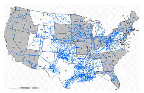
Figure 1.
The interstate US pipeline natural gas network (Source: Energy Information Administration, Office of Oil and Gas, Natural Gas Division, Gas Transportation Information System, http://www.eia.doe.gov/pub/oil_gas/natural_gas/analysis_publications/ngpipeline/dependstates_map.html).
4.1. Data and Variables
Annual data relative to the flow of natural gas from state to state along the US interstate gas pipelines were retrieved from the EIA database for the period 2013–2017 [65]. These data were used to assemble the adjacency matrix relative to the gas network for every year. The following SNA centrality metrics were calculated for every matrix: In-degree, out-degree, emission degree, reception degree, flow betweenness, and sociometric status. Because of the high correlation between the emission degree and the sociometric status, the latter was omitted from the analysis. The basic network statistics are provided in Table 2. Figure 2 shows the representation of the interstate US natural gas infrastructure as a graph. Table 3 displays the mean and maximum values relative to SNA indexes from 2013 to 2017. As the data show, both the mean and maximum values increased from 2013 to 2017 for all indexes.
Table 2.
Basic network statistics for the interstate US gas transmission infrastructure.
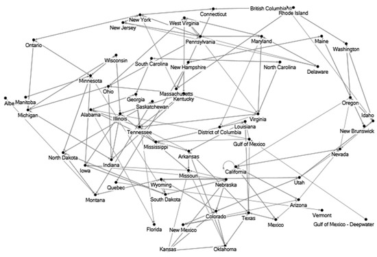
Figure 2.
Graph of the interstate US gas transmission infrastructure network.
Table 3.
Mean and maximum values of SNA indexes.
4.2. Cross-Efficiency DEA Model Specification
Two cross-efficiency DEA model specifications were used to aggregate SNA indexes and rank network nodes, the first one evaluating each node from the supply-side perspective and the second one evaluating it from the demand-side perspective. Two different sets of SNA indexes were chosen as input and output variables for every model to perform DEA. Table 4 shows the input and output variables for both models. The demand-side DEA model utilizes the in-degree and the reception degree indexes as the only input and output, respectively. It was assumed that a node is more critical than others in the network if it receives a higher amount of gas. However, given the same amount of gas received by nodes, if one of them receives gas from several nodes, the latter is less critical than the others. Indeed, it is assumed that redundancy decreases local vulnerability from the demand-side perspective. In the supply-side DEA model, three outputs from the set of SNA indexes are used, e.g., emission degree, out-degree, and flow betweenness. From the supply-side, it is assumed that the greater the number of nodes to which a node supplies gas and the greater the amount of gas it supplies is, the more critical that node is in the network. Furthermore, the more the node contributes to the volume of gas transmitted in the network, the more critical it is. For all DMUs, a constant factor having a measurement equal to one was included in the model specification as an input.
Table 4.
Input and output variables.
In both DEA models, constant returns to scale and output orientation were used to solve Equation (2). The two indexes were aggregated to have an overall cross-efficiency measurement using the Shannon’s entropy index to generate weights applying the procedure suggested in the literature [66,67,68].
4.3. Results
In this section, results from the implementation of the SNA-DEA prioritization method for the US interstate gas industry are presented. Higher cross-efficiency scores indicate more critical nodes in the network.
Figure 3 illustrates changes in the cross-efficiency mean values relative to the whole network from 2013 to 2017. Cross-efficiencies were computed from both perspectives of the supply side and demand side. The overall cross-efficiency measurement was obtained as the weighted average of the two previous cross-efficiencies utilizing the set of weights generated through the Shannon’s entropy index procedure. For the sake of brevity, the list of weights was not included in the paper.
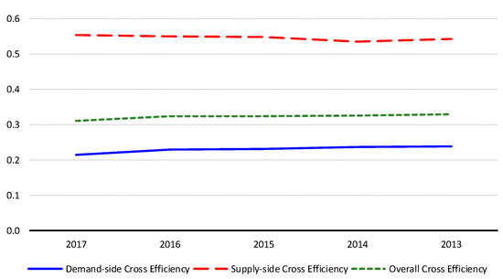
Figure 3.
Cross-efficiency mean values.
From the demand-side perspective, the cross-efficiency mean value was slightly diminished from 2013 to 2017, even though the average reception degree increased by roughly 15%. On the contrary, from the supply-side perspective, there was a small increase of the cross-efficiency mean score from 2013 to 2017. These findings indicate that the topological characteristics of the US interstate gas network did not substantially change over time from 2013 to 2017 with respect to major critical nodes.
Figure 4, Figure 5, Figure 6, Figure 7 and Figure 8 show the outcome of a more in-depth analysis of the cross-efficiency measurements. For every year, the cross-efficiency scores relative to all nodes are reported. Table A1 in the Appendix A presents all cross-efficiency measurements. From the demand-side perspective, only one node—NO21 (Louisiana State)—achieves a 100% cross-efficiency score, ranking the state of Louisiana in first place as the most critical node in the network. The cross-efficiency score of the node NO29 (Mississippi State) is between 0.758 and 0.776. This node ranks in second place. As already mentioned, there was a little change over the years, and only for a few nodes of the network were there appreciable cross-efficiency variations. That is the case of South Carolina state (node NO49), whose cross-efficiency score decreased from 0.524 to 0.259. When network nodes are assessed from the supply-side perspective, the cross-efficiency analysis identifies a larger number of critical nodes. In 2017, four nodes—NO7, NO20, NO45, and NO51 (Colorado, Kentucky, Pennsylvania, Tennessee)—achieve a cross-efficiency value between 0.999 and 1. These nodes are the most critical ones from the supply perspective. However, there is a great number of nodes achieving remarkable cross-efficiency measurements, such as the states of Arkansas (0.831), Illinois (0.831), Maryland (0.830), Minnesota (0.832), Nebraska (0.830), New York (0.867), Ohio (0.830), Oklahoma (0.833), South Dakota (0.828), Texas (0.888), West Virginia (0.830), and Wyoming (0.832). As in the demand-side perspective, there has not been a significant change in the cross-efficiency scores of individual nodes during the time period under investigation, except for a restricted number of nodes, such as Georgia (NO12) and Mississippi (NO29), whose cross-efficiencies passed from 0.497 to 0.664 and from 0.593 to 0.726 in 2013 and in 2017, respectively. Generally, cross-efficiency measurements tend to be very similar from year to year as interstate gas flows remained almost unchanged from 2013 to 2017.
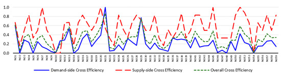
Figure 4.
Cross-efficiency scores, year 2017.
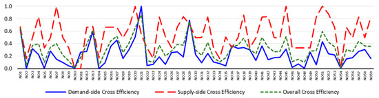
Figure 5.
Cross-efficiency scores, year 2016.
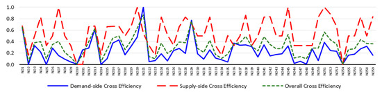
Figure 6.
Cross-efficiency scores, year 2015.
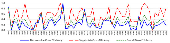
Figure 7.
Cross-efficiency scores, year 2014.
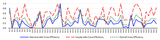
Figure 8.
Cross-efficiency scores, year 2013.
Figure 9, Figure 10 and Figure 11 display the ranking of network nodes using a histogram graph. On the vertical axis of the graph, cross-efficiency scores are reported. The bars are placed on the graph in rank order. Thus, bars at the left side have the highest cross-efficiency score. The graphical analysis was restricted to year 2017 only. The results clearly show that the influence of a node is not equal from the two different perspectives that were adopted to assess the network. Indeed, the ranking of network nodes in Figure 9 significantly differs from the ranking in Figure 10. That supports the idea that it is necessary to collect information and assess the gas network from different perspectives to gain an in-depth understanding of its capacity and performance, and finally identify critical nodes. Additionally, the different rankings provided by the two assessment perspectives suggest that the supply-side perspective appears more critical than the demand-side one.
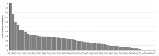
Figure 9.
Ranking of network nodes (demand-side perspective).
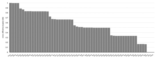
Figure 10.
Ranking of network nodes (supply-side perspective).
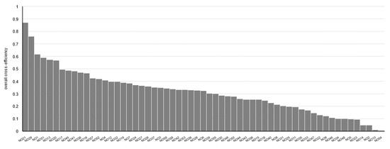
Figure 11.
Ranking of network nodes (overall cross-efficiency measurement).
5. Conclusions
In this paper, a prioritization framework to uncover the critical nodes of gas pipeline networks was proposed. This method considers the topological characteristics of the network and calculates a set of metrics typical of the social network analysis. Finally, these metrics were used as input and output variables of a data envelopment analysis model to measure a cross-efficiency index, which identified the most influencing nodes in the network. Cross-efficiency DEA allows nodes in the network to be easily ranked. The framework was implemented to study the US interstate gas network between 2013 and 2017 from the demand- and supply-side perspectives. A comprehensive score to prioritize the infrastructure nodes was obtained using the Shannon’s entropy index. The aggregating procedure based on the Shannon’s entropy index allowed the node rankings obtained to be merged assuming different perspectives, providing a Pareto optimal solution that was better than averaging individual ranking scores [67].
The findings of this study confirm that it is necessary to consider different perspectives in the analysis of gas networks. Indeed, adopting the two assessment perspectives’ different nodes of the US interstate gas pipelines network emerged as being important and critical. That means that the elements of the network that have relevance for ensuring supply stability in transmitting gas from a node to other nodes do not always have relevance as the elements that are necessary for assuring local gas availability.
As the main purpose of this paper was to illustrate the evaluation framework, the presentation of results relative to the investigation of the US gas infrastructure criticalities was restricted only to five years for the sake of brevity and to avoid making the analysis cumbersome. On the other hand, a full study covering the time period from 2007 to 2017 revealed that there have not been significant changes.
Of course, although the information provided by such a framework is important for the preliminary assessment of gas pipeline networks and the identification of critical nodes, a more comprehensive assessment of the gas network capacity and performance should employ complementary methods, including further information, such as the number of gas pipeline operators, their operational integrity, and ability to recover rapidly after supply interruption; the impact of any prolonged infrastructure downtime; the storage facility capacity; local gas demand; and infrastructure reliability level, in the analysis.
The proposed framework can be easily applied to the assessment of other pipeline industries or similar infrastructure systems if the characteristics of the network are taken into account. Information provided by the implementation of this method can be important for the operation and improvement of the network (i.e., maintenance, new branch construction), design, and planning. The same method can be extended to the assessment of the edges of the network (e.g., the pipelines).
In this paper, the framework only considered the basic structural characteristics of the US interstate natural gas infrastructure as a graph, focusing on the connectivity properties of the network. The assessment of the critical nodes of the network assumed that its vulnerability is correlated to some structural features of the network. Of course, this view is reductive as the hydro-thermal characteristics of natural gas that impose constraints on pipeline operation were not considered in the analysis. Natural gas transportation infrastructure is sensitive to gas quality, thermodynamic properties, and physical features (e.g., its low volumetric energy density, minimum delivery pressures at offtake points, maximum operating pipeline pressures, maximum available compression power, etc.), and storage difficulties make it difficult to alleviate supply shocks. However, the proposed framework is scalable and flexible, and it can be expanded and improved in many directions in the future. Particularly, it can integrate data from fluid dynamics models, providing a more accurate model of the natural gas system. For instance, in order to take into account constraints related to the capacity of nodes that supply gas and transmission links, the max-flow betweenness centrality index might be included in Equations (2) and (3) rather than the flow betweenness index, as in Fang and Zio [69]. Quality metrics of the gas flow stream can also be included as further outputs in Equation (3). Additionally, several time-dependent scenarios can be constructed to follow the evolution of the gas network over time, thus detecting which nodes and links change, when these changes occur, and evaluating the impact this might have on the topological structure while performing the analysis within a discrete time domain. The SNA literature provides suggestions on how to measure network centrality indexes accounting for the influence of time [70,71].
Funding
This research received no external funding.
Acknowledgments
I thank the anonymous reviewers for their careful reading of my manuscript and their insightful comments and suggestions.
Conflicts of Interest
The author declares no conflict of interest.
Appendix A
Table A1.
Cross-efficiency measurements.
Table A1.
Cross-efficiency measurements.
| Node | State | 2017 | 2016 | 2015 | 2014 | 2013 | ||||||||||
|---|---|---|---|---|---|---|---|---|---|---|---|---|---|---|---|---|
| D | S | OE | D | S | OE | D | S | OE | D | S | OE | D | S | OE | ||
| NO1 | Alabama | 0.595 | 0.670 | 0.616 | 0.631 | 0.670 | 0.643 | 0.644 | 0.672 | 0.652 | 0.860 | 0.680 | 0.807 | 0.815 | 0.680 | 0.775 |
| NO2 | Alberta | 0.000 | 0.165 | 0.047 | 0.000 | 0.166 | 0.048 | 0.000 | 0.166 | 0.049 | 0.000 | 0.164 | 0.049 | 0.000 | 0.165 | 0.049 |
| NO3 | Arizona | 0.289 | 0.498 | 0.349 | 0.322 | 0.498 | 0.373 | 0.333 | 0.498 | 0.381 | 0.347 | 0.495 | 0.391 | 0.352 | 0.497 | 0.395 |
| NO4 | Arkansas | 0.240 | 0.831 | 0.409 | 0.228 | 0.831 | 0.404 | 0.223 | 0.831 | 0.401 | 0.262 | 0.827 | 0.430 | 0.266 | 0.829 | 0.433 |
| NO5 | British Columbia | 0.005 | 0.332 | 0.098 | 0.005 | 0.332 | 0.100 | 0.005 | 0.332 | 0.101 | 0.005 | 0.330 | 0.102 | 0.006 | 0.331 | 0.102 |
| NO6 | California | 0.252 | 0.500 | 0.323 | 0.280 | 0.499 | 0.344 | 0.289 | 0.499 | 0.351 | 0.324 | 0.497 | 0.375 | 0.306 | 0.497 | 0.363 |
| NO7 | Colorado | 0.138 | 0.997 | 0.384 | 0.154 | 0.997 | 0.400 | 0.159 | 0.997 | 0.405 | 0.165 | 0.992 | 0.411 | 0.172 | 0.995 | 0.417 |
| NO8 | Connecticut | 0.096 | 0.510 | 0.214 | 0.104 | 0.506 | 0.222 | 0.096 | 0.506 | 0.216 | 0.100 | 0.501 | 0.219 | 0.101 | 0.501 | 0.220 |
| NO9 | Delaware | 0.039 | 0.331 | 0.122 | 0.043 | 0.331 | 0.127 | 0.045 | 0.331 | 0.129 | 0.041 | 0.328 | 0.126 | 0.028 | 0.329 | 0.118 |
| NO10 | District of Columbia | 0.012 | 0.001 | 0.009 | 0.013 | 0.001 | 0.009 | 0.008 | 0.001 | 0.006 | 0.014 | 0.001 | 0.010 | 0.014 | 0.001 | 0.010 |
| NO11 | Florida | 0.272 | 0.001 | 0.195 | 0.262 | 0.001 | 0.186 | 0.259 | 0.001 | 0.183 | 0.270 | 0.001 | 0.190 | 0.274 | 0.001 | 0.193 |
| NO12 | Georgia | 0.289 | 0.664 | 0.396 | 0.279 | 0.664 | 0.391 | 0.288 | 0.664 | 0.398 | 0.282 | 0.495 | 0.345 | 0.286 | 0.497 | 0.349 |
| NO13 | Gulf of Mexico | 0.534 | 0.672 | 0.574 | 0.595 | 0.675 | 0.618 | 0.615 | 0.676 | 0.633 | 0.640 | 0.680 | 0.652 | 0.650 | 0.691 | 0.662 |
| NO14 | Gulf of Mexico Deepwater | 0.000 | 0.168 | 0.048 | 0.000 | 0.169 | 0.049 | 0.000 | 0.169 | 0.050 | 0.000 | 0.170 | 0.051 | 0.000 | 0.173 | 0.051 |
| NO15 | Idaho | 0.088 | 0.663 | 0.253 | 0.098 | 0.663 | 0.263 | 0.101 | 0.663 | 0.266 | 0.105 | 0.659 | 0.270 | 0.107 | 0.661 | 0.271 |
| NO16 | Illinois | 0.320 | 0.831 | 0.466 | 0.356 | 0.666 | 0.447 | 0.377 | 0.665 | 0.461 | 0.341 | 0.662 | 0.436 | 0.346 | 0.666 | 0.441 |
| NO17 | Indiana | 0.425 | 0.666 | 0.494 | 0.459 | 0.666 | 0.520 | 0.434 | 0.666 | 0.502 | 0.405 | 0.662 | 0.481 | 0.411 | 0.664 | 0.486 |
| NO18 | Iowa | 0.146 | 0.498 | 0.247 | 0.162 | 0.498 | 0.261 | 0.168 | 0.498 | 0.265 | 0.175 | 0.496 | 0.270 | 0.177 | 0.498 | 0.272 |
| NO19 | Kansas | 0.278 | 0.666 | 0.389 | 0.309 | 0.665 | 0.413 | 0.320 | 0.665 | 0.421 | 0.333 | 0.662 | 0.431 | 0.347 | 0.663 | 0.441 |
| NO20 | Kentucky | 0.393 | 0.999 | 0.567 | 0.505 | 0.999 | 0.650 | 0.483 | 0.999 | 0.634 | 0.412 | 0.997 | 0.586 | 0.418 | 0.998 | 0.590 |
| NO21 | Louisiana | 1.000 | 0.545 | 0.870 | 1.000 | 0.547 | 0.868 | 1.000 | 0.549 | 0.868 | 1.000 | 0.571 | 0.873 | 1.000 | 0.584 | 0.877 |
| NO22 | Maine | 0.048 | 0.333 | 0.129 | 0.053 | 0.332 | 0.135 | 0.055 | 0.332 | 0.136 | 0.058 | 0.331 | 0.139 | 0.058 | 0.331 | 0.139 |
| NO23 | Manitoba | 0.063 | 0.166 | 0.093 | 0.071 | 0.166 | 0.098 | 0.073 | 0.166 | 0.100 | 0.076 | 0.165 | 0.102 | 0.077 | 0.166 | 0.103 |
| NO24 | Maryland | 0.185 | 0.830 | 0.369 | 0.189 | 0.830 | 0.376 | 0.187 | 0.830 | 0.376 | 0.183 | 0.826 | 0.374 | 0.186 | 0.827 | 0.376 |
| NO25 | Massachusetts | 0.065 | 0.522 | 0.196 | 0.072 | 0.517 | 0.202 | 0.066 | 0.517 | 0.198 | 0.069 | 0.524 | 0.204 | 0.070 | 0.519 | 0.203 |
| NO26 | Mexico | 0.322 | 0.342 | 0.328 | 0.256 | 0.339 | 0.280 | 0.245 | 0.339 | 0.272 | 0.250 | 0.337 | 0.276 | 0.163 | 0.338 | 0.215 |
| NO27 | Michigan | 0.245 | 0.664 | 0.365 | 0.273 | 0.664 | 0.387 | 0.282 | 0.664 | 0.394 | 0.294 | 0.660 | 0.403 | 0.299 | 0.662 | 0.407 |
| NO28 | Minnesota | 0.169 | 0.832 | 0.359 | 0.188 | 0.831 | 0.376 | 0.195 | 0.832 | 0.382 | 0.203 | 0.827 | 0.388 | 0.206 | 0.830 | 0.391 |
| NO29 | Mississippi | 0.772 | 0.726 | 0.759 | 0.776 | 0.717 | 0.759 | 0.771 | 0.715 | 0.755 | 0.770 | 0.584 | 0.715 | 0.758 | 0.593 | 0.709 |
| NO30 | Missouri | 0.202 | 0.497 | 0.287 | 0.225 | 0.498 | 0.305 | 0.192 | 0.498 | 0.281 | 0.199 | 0.495 | 0.287 | 0.202 | 0.497 | 0.290 |
| NO31 | Montana | 0.084 | 0.501 | 0.203 | 0.093 | 0.499 | 0.212 | 0.096 | 0.499 | 0.215 | 0.100 | 0.496 | 0.218 | 0.102 | 0.498 | 0.219 |
| NO32 | Nebraska | 0.222 | 0.830 | 0.396 | 0.248 | 0.830 | 0.418 | 0.256 | 0.830 | 0.424 | 0.267 | 0.825 | 0.432 | 0.284 | 0.827 | 0.445 |
| NO33 | Nevada | 0.099 | 0.333 | 0.166 | 0.110 | 0.332 | 0.175 | 0.113 | 0.333 | 0.178 | 0.118 | 0.167 | 0.133 | 0.120 | 0.332 | 0.183 |
| NO34 | New Brunswick | 0.074 | 0.166 | 0.100 | 0.082 | 0.166 | 0.107 | 0.085 | 0.166 | 0.109 | 0.089 | 0.164 | 0.111 | 0.090 | 0.165 | 0.112 |
| NO35 | New Hampshire | 0.039 | 0.512 | 0.175 | 0.044 | 0.508 | 0.179 | 0.045 | 0.508 | 0.181 | 0.047 | 0.505 | 0.183 | 0.048 | 0.504 | 0.183 |
| NO36 | New Jersey | 0.329 | 0.332 | 0.330 | 0.362 | 0.333 | 0.354 | 0.375 | 0.332 | 0.362 | 0.384 | 0.331 | 0.368 | 0.365 | 0.332 | 0.355 |
| NO37 | New Mexico | 0.292 | 0.498 | 0.351 | 0.325 | 0.498 | 0.375 | 0.336 | 0.498 | 0.383 | 0.350 | 0.496 | 0.393 | 0.355 | 0.497 | 0.397 |
| NO38 | New York | 0.310 | 0.867 | 0.469 | 0.339 | 0.858 | 0.491 | 0.342 | 0.858 | 0.493 | 0.352 | 0.861 | 0.503 | 0.354 | 0.856 | 0.503 |
| NO39 | North Carolina | 0.291 | 0.333 | 0.303 | 0.302 | 0.332 | 0.311 | 0.312 | 0.332 | 0.318 | 0.292 | 0.175 | 0.257 | 0.272 | 0.168 | 0.241 |
| NO40 | North Dakota | 0.117 | 0.499 | 0.226 | 0.131 | 0.498 | 0.238 | 0.135 | 0.499 | 0.242 | 0.074 | 0.495 | 0.199 | 0.143 | 0.497 | 0.248 |
| NO41 | Ohio | 0.341 | 0.830 | 0.481 | 0.367 | 0.830 | 0.502 | 0.347 | 0.830 | 0.489 | 0.340 | 0.828 | 0.485 | 0.325 | 0.828 | 0.475 |
| NO42 | Oklahoma | 0.133 | 0.833 | 0.333 | 0.148 | 0.832 | 0.347 | 0.153 | 0.832 | 0.352 | 0.159 | 0.662 | 0.308 | 0.161 | 0.831 | 0.360 |
| NO43 | Ontario | 0.156 | 0.498 | 0.254 | 0.174 | 0.498 | 0.269 | 0.180 | 0.498 | 0.273 | 0.177 | 0.495 | 0.272 | 0.180 | 0.496 | 0.274 |
| NO44 | Oregon | 0.165 | 0.499 | 0.260 | 0.183 | 0.499 | 0.275 | 0.189 | 0.499 | 0.280 | 0.197 | 0.498 | 0.286 | 0.200 | 0.497 | 0.288 |
| NO45 | Pennsylvania | 0.281 | 0.999 | 0.486 | 0.312 | 1.000 | 0.513 | 0.323 | 1.000 | 0.521 | 0.336 | 0.997 | 0.533 | 0.337 | 0.998 | 0.533 |
| NO46 | Quebec | 0.019 | 0.332 | 0.109 | 0.021 | 0.331 | 0.112 | 0.022 | 0.331 | 0.113 | 0.023 | 0.329 | 0.114 | 0.023 | 0.330 | 0.114 |
| NO47 | Rhode Island | 0.069 | 0.334 | 0.145 | 0.077 | 0.333 | 0.151 | 0.062 | 0.333 | 0.141 | 0.064 | 0.331 | 0.144 | 0.065 | 0.331 | 0.144 |
| NO48 | Saskatchewan | 0.007 | 0.331 | 0.100 | 0.008 | 0.332 | 0.103 | 0.008 | 0.332 | 0.103 | 0.009 | 0.330 | 0.104 | 0.009 | 0.331 | 0.104 |
| NO49 | South Carolina | 0.259 | 0.333 | 0.280 | 0.266 | 0.332 | 0.285 | 0.275 | 0.333 | 0.292 | 0.516 | 0.331 | 0.461 | 0.524 | 0.332 | 0.467 |
| NO50 | South Dakota | 0.060 | 0.828 | 0.279 | 0.066 | 0.828 | 0.289 | 0.068 | 0.828 | 0.291 | 0.071 | 0.822 | 0.294 | 0.072 | 0.825 | 0.296 |
| NO51 | Tennessee | 0.424 | 1.000 | 0.589 | 0.432 | 1.000 | 0.598 | 0.390 | 1.000 | 0.569 | 0.373 | 1.000 | 0.559 | 0.359 | 1.000 | 0.550 |
| NO52 | Texas | 0.233 | 0.888 | 0.420 | 0.238 | 0.879 | 0.425 | 0.246 | 0.879 | 0.431 | 0.171 | 0.892 | 0.385 | 0.268 | 0.896 | 0.455 |
| NO53 | Utah | 0.198 | 0.665 | 0.332 | 0.222 | 0.665 | 0.352 | 0.230 | 0.665 | 0.357 | 0.239 | 0.662 | 0.365 | 0.243 | 0.663 | 0.368 |
| NO54 | Vermont | 0.006 | 0.001 | 0.004 | 0.006 | 0.001 | 0.005 | 0.006 | 0.001 | 0.005 | 0.007 | 0.001 | 0.005 | 0.007 | 0.001 | 0.005 |
| NO55 | Virginia | 0.152 | 0.665 | 0.299 | 0.159 | 0.665 | 0.306 | 0.164 | 0.499 | 0.262 | 0.162 | 0.663 | 0.310 | 0.164 | 0.663 | 0.312 |
| NO56 | Washington | 0.156 | 0.498 | 0.254 | 0.174 | 0.498 | 0.269 | 0.180 | 0.498 | 0.273 | 0.187 | 0.495 | 0.279 | 0.190 | 0.496 | 0.281 |
| NO57 | West Virginia | 0.263 | 0.830 | 0.425 | 0.277 | 0.831 | 0.438 | 0.277 | 0.830 | 0.439 | 0.239 | 0.825 | 0.413 | 0.206 | 0.828 | 0.390 |
| NO58 | Wisconsin | 0.275 | 0.498 | 0.339 | 0.307 | 0.498 | 0.362 | 0.317 | 0.498 | 0.370 | 0.330 | 0.495 | 0.379 | 0.335 | 0.496 | 0.383 |
| NO59 | Wyoming | 0.145 | 0.832 | 0.342 | 0.162 | 0.832 | 0.357 | 0.167 | 0.832 | 0.362 | 0.174 | 0.828 | 0.368 | 0.176 | 0.831 | 0.371 |
Note: D = Demand-side; S = Supply-side; OE = Overall efficiency.
References
- US Energy Information Administration. Monthly Energy Review. June 2019. Available online: https://www.eia.gov/totalenergy/data/monthly/archive/00351906.pdf (accessed on 15 October 2019).
- US Energy Information Administration. International Energy Outlook 2016. Available online: https://www.eia.gov/outlooks/ieo/pdf/0484(2016).pdf (accessed on 15 October 2019).
- Koç, Y.; Warnier, M.; Kooij, R.; Brazier, F. Structural vulnerability assessment of electric power grids. In Proceedings of the 11th IEEE International Conference on Networking, Sensing and Control (ICNSC), Miami, FL, USA, 7–9 April 2014; pp. 386–391. Available online: https://ieeexplore.ieee.org/document/6819657 (accessed on 17 October 2019).
- Fichera, A.; Frasca, M.; Volpe, R. Complex networks for the integration of distributed energy systems in urban areas. Appl. Energy 2017, 193, 336–345. [Google Scholar] [CrossRef]
- Qiao, Z.; Guo, Q.; Sun, H.; Pan, Z.; Liu, Y.; Xiong, W. An interval gas flow analysis in natural gas and electricity coupled networks considering the uncertainty of wind power. Appl. Energy 2017, 201, 343–353. [Google Scholar] [CrossRef]
- Chertikov, M.; Backhaus, S.; Lebedev, V. Cascading of fluctuations in interdependent energy infrastructures: Gas-grid coupling. Appl. Energy 2016, 160, 541–551. [Google Scholar] [CrossRef]
- Su, H.; Zhang, J.; Zio, E.; Yang, N.; Li, X.; Zhang, Z. An integrated system method for supply reliability assessment of natural gas pipeline networks. Appl. Energy 2018, 209, 489–501. [Google Scholar] [CrossRef]
- Ouyang, M. Review on modeling and simulation of interdependent critical infrastructure systems. Reliab. Eng. Syst. Saf. 2014, 121, 43–60. [Google Scholar] [CrossRef]
- Kizhakkedath, A.; Tai, K.; Sim, M.S.; Tiong, R.L.K.; Lin, J. An Agent-Based Modeling and Evolutionary Optimization Approach for Vulnerability Analysis of Critical Infrastructure Networks. In AsiaSim 2013. Communications in Computer and Information Science; Tan, G., Yeo, G.K., Turner, S.J., Teo, Y.M., Eds.; Springer: Berlin/Heidelberg, Germany, 2013; Volume 402. [Google Scholar]
- Subramanian, A.S.R.; Gundersen, T.; Adams, T.A., II. Modeling and Simulation of Energy Systems: A Review. Processes 2018, 6, 238. [Google Scholar] [CrossRef]
- Behrooz, H.A.; Boozarjomehry, R.B. Dynamic optimization of natural gas networks under customer demand uncertainties. Energy 2017, 134, 968–983. [Google Scholar] [CrossRef]
- Fu, X.; Guo, Q.; Sun, H.; Zhang, X.; Wang, L. Estimation of the failure probability of an integrated energy system based on the first order reliability method. Energy 2017, 134, 1068–1078. [Google Scholar] [CrossRef]
- Correa-Posada, C.M.; Sanchez-Martin, P.; Lumbreras, S. Security-constrained model for integrated power and natural-gas system. J. Modeling Power Syst. Clean Energy 2017, 5, 326–336. [Google Scholar] [CrossRef]
- Rehak, D.; Senovsky, P.; Hromada, M.; Lovecek, T. Complex approach to assessing resilience of critical infrastructure elements. Int. J. Crit. Infrastruct. Prot. 2019, 25, 125–138. [Google Scholar] [CrossRef]
- Monforti, F.; Szikszai, A. A Monte-Carlo approach for assessing the adequacy of the European gas transmission system under supply crisis conditions. Energy Policy 2010, 38, 2486–2498. [Google Scholar] [CrossRef]
- Chaudry, M.; Wu, J.; Jenkins, N. A sequential Monte Carlo model of the combined GB gas and electricity network. Energy Policy 2013, 62, 473–483. [Google Scholar] [CrossRef]
- Nan, C.; Sansavini, G. A quantitative method for assessing resilience of interdependent infrastructures. Reliab. Eng. Syst. Saf. 2017, 157, 35–53. [Google Scholar] [CrossRef]
- Voropai, N.I.; Senderov, S.M.; Edelev, A.V. Detection of “bottlenecks” and ways to overcome emergency situations in gas transportation networks on the example of the European gas pipeline network. Energy 2012, 42, 3–9. [Google Scholar] [CrossRef]
- Ouyang, M. Critical location identification and vulnerability analysis of interdependent infrastructure systems under spatially localized attacks. Reliab. Eng. Syst. Saf. 2016, 154, 106–116. [Google Scholar] [CrossRef]
- Shaikh, F.; Ji, Q.; Ying, F. Evaluating China’s natural gas supply security based on ecological network analysis. J. Clean. Prod. 2016, 139, 1196–1206. [Google Scholar] [CrossRef]
- Cetinay, H.; Devriendt, K.; Van Mieghem, P. Nodal vulnerability to targeted attacks in power grids. Appl. Netw. Sci. 2018, 3, 34. [Google Scholar] [CrossRef]
- Beyza, J.; Garcia-Paricio, E.; Yusta, J.M. Applying Complex Network Theory to the Vulnerability Assessment of Interdependent Energy Infrastructures. Energies 2019, 12, 421. [Google Scholar] [CrossRef]
- Beyza, J.; Rui-Paredes, H.F.; Garcia-Paricio, E.; Yusta, J.M. Assessing the criticality of interdependent power and gas systems using complex networks and load flow techniques. Phys. A Stat. Mech. Appl. 2020, 540, 123169. [Google Scholar] [CrossRef]
- Zio, E. Challenges in the vulnerability and risk analysis of critical infrastructures. Reliab. Eng. Syst. Saf. 2016, 152, 137–150. [Google Scholar] [CrossRef]
- Han, F.; Zio, E. A multi-perspective framework of analysis of critical infrastructures with respect to supply service, controllability and topology. Int. J. Crit. Infrastruct. Prot. 2019, 24, 1–13. [Google Scholar] [CrossRef]
- Alipour, Z.; Monfared, M.A.S.; Enrico Zio, E. Comparing topological and reliability-based vulnerability analysis of Iran power transmission network. Proc. Inst. Mech. Eng. Part O J. Risk Reliab. 2014, 228, 139–151. [Google Scholar] [CrossRef]
- Praks, P.; Kopustinskas, V.; Masera, M. Probabilistic modelling of security of supply in gas networks and evaluation of new infrastructure. Reliab. Eng. Syst. Saf. 2015, 144, 254–264. [Google Scholar] [CrossRef]
- Su, H.; Zio, E.; Zhang, J.; Xueyi, L. A systematic framework of vulnerability analysis of a natural gas pipeline network. Reliab. Eng. Syst. Saf. 2018, 175, 79–91. [Google Scholar] [CrossRef]
- Hanneman, R.A.; Riddle, M. Introduction to Social Network Methods; University of California: Riverside, CA, USA, 2005. [Google Scholar]
- Wasserman, S.; Faust, K. Social Network Analysis; Cambridge University Press: Cambridge, MA, USA, 1994. [Google Scholar]
- Watts, D.J. The “New” science of networks. Annu. Rev. Sociol. 2004, 30, 243–270. [Google Scholar] [CrossRef]
- Willging, P.A. Using Social Network Analysis Techniques to Examine Online Interactions. US China Educ. Rev. 2005, 2, 46–56. [Google Scholar]
- Barabasi, A.L.; Albert, R.; Jeong, H.; Bianconi, G. Power-Law distribution of the World Wide Web. Science 2000, 287, 2115. [Google Scholar]
- lo Storto, C. Investigating information flows across complex product development stages by using social network analysis (SNA). In Proceedings of the COMPENG 2010, Rome, Italy, 22–24 February 2010; ISBN 978-0-7695-3974-4. [Google Scholar]
- lo Storto, C. A four-stage framework for the identification of information flow inefficiencies in the manufacturing environment. Appl. Mech. Mater. 2013, 309, 335–341. [Google Scholar] [CrossRef]
- Pastor-Satorras, R.; Vespignani, A. Epidemic spreading in scale-free networks. Phys. Rev. Lett. 2001, 86, 3200–3203. [Google Scholar] [CrossRef]
- Newman, M.E.J. The Structure and Function of Complex Networks. SIAM Rev. 2003, 45, 167–256. [Google Scholar] [CrossRef]
- Allen, J.; James, A.D.; Gamlen, P. Formal versus informal knowledge networks in R&D: A case study using social network analysis. R D Manag. 2007, 37, 179–196. [Google Scholar]
- Weiwei, L.; Yuan, T.; Zhile, Y.; Kexin, B. Exploring and Visualizing the Patent Collaboration Network: A Case Study of Smart Grid Field in China. Sustainability 2019, 11, 465. [Google Scholar]
- Uzzi, B.; Spiro, J. Collaboration and Creativity: The Small World Problem. Am. J. Sociol. 2005, 111, 447–504. [Google Scholar] [CrossRef]
- Zanin, M.; Lillo, F. Modelling the air transport with complex networks: A short review. Eur. Phys. J. Spec. Top. 2013, 215, 5–21. [Google Scholar] [CrossRef]
- Son, M.G.; Yeo, G.T. Analysis of the Air Transport Network Characteristics of Major Airports. Asian J. Shipp. Logist. 2017, 33, 117–125. [Google Scholar]
- Barrat, A.; Barthélemy, M.; Pastor-Satorras, R.; Vespignani, A. The architecture of complex weighted networks. PNAS 2004, 101, 3747–3752. [Google Scholar] [CrossRef]
- Iyengar, D.; Rao, S.; Goldsby, T.J. The Power and Centrality of the Transportation and Warehousing Sector within the US Economy: A Longitudinal Exploration Using Social Network Analysis. Transp. J. 2012, 51, 373–398. [Google Scholar] [CrossRef]
- Saleh, M.; Esa, Y.; Mohamed, A. Applications of Complex Network Analysis in Electric Power Systems. Energies 2018, 11, 1381. [Google Scholar] [CrossRef]
- Watts, D.J.; Strogatz, S.H. Collective dynamics of “small-world” networks. Nature 1998, 393, 440–442. [Google Scholar] [CrossRef]
- Zhao, J.; Zhou, H.; Chen, B.; Li, P. Research on the structural characteristics of transmission grid based on complex network theory. J. Appl. Math. 2014, 2014. [Google Scholar] [CrossRef][Green Version]
- Piccinelli, R.; Krausmann, E. An Analysis of the Vulnerability of Power Grids to Extreme Space Weather Using Complex Network Theory; Technical Report, European Commission Joint Research Center; Institute for the Protection and Security of the Citizen: Ispra, Italy, 2015; Available online: http://publications.jrc.ec.europa.eu/repository/handle/JRC91072 (accessed on 18 October 2019).
- Bonacich, P. Power and Centrality: A family of measures. Am. J. Sociol. 1987, 92, 1170–1182. [Google Scholar] [CrossRef]
- Borgatti, S.P. Centrality and network flow. Soc. Netw. 2005, 27, 55–71. [Google Scholar] [CrossRef]
- Freeman, L.C. Centrality in social networks conceptual clarification. Soc. Netw. 1978, 1, 215–239. [Google Scholar] [CrossRef]
- Newman, M.E.J. A measure of betweenness centrality based on random walks. Soc. Netw. 2005, 27, 39–54. [Google Scholar] [CrossRef]
- Freeman, L.C.; Borgatti, S.P.; White, D.R. Centrality in valued graphs: A measure of betweenness based on network flow. Soc. Netw. 1991, 13, 141–154. [Google Scholar] [CrossRef]
- Houghton, R.J.; Baber, C.; McMaster, R.; Stanton, N.A.; Salmon, P.; Stewart, R.; Walker, G.H. Command and control in emergency services operations: A social network analysis. Ergonomics 2006, 49, 1204–1225. [Google Scholar] [CrossRef]
- Tapiero, C.S.; Lewin, A.Y. The Concept and Measurement of Centrality–An Information Approach. Decis. Sci. 1973, 4, 314–328. [Google Scholar] [CrossRef]
- Cooper, W.W.; Seiford, L.M.; Tone, K. Data Envelopment Analysis: A Comprehensive Text with Models, Applications, References and DEA-Solver Software, 2nd ed.; Springer: Berlin, Germany, 2006. [Google Scholar]
- Charnes, A.; Cooper, W.W.; Rhodes, E. Measuring the efficiency of decision-making units. Eur. J. Oper. Res. 1989, 2, 429–444. [Google Scholar] [CrossRef]
- Noorizadeh, A.; Mahdiloo, M.; Saen, R.F. Using DEA Cross-efficiency Evaluation for Suppliers Ranking in the Presence of Non-discretionary Inputs. Int. J. Shipp. Transp. Logist. 2013, 5, 95–111. [Google Scholar] [CrossRef]
- Sexton, T.R.; Silkman, R.H.; Hogan, A.J. Data envelopment analysis: Critique and extensions. In Measuring Efficiency: An Assessment of Data Envelopment Analysis; Silkman, R.H., Ed.; Jossey-Bass: New York, NY, USA, 1986; pp. 73–105. [Google Scholar]
- Doyle, J.R.; Green, R.H. Efficiency and cross-efficiency in DEA: Derivations, meanings and uses. J. Oper. Res. Soc. 1994, 45, 567–578. [Google Scholar] [CrossRef]
- lo Storto, C. A double-DEA framework to support decision-making in the choice of advanced manufacturing technologies. Manag. Decis. 2018, 56, 488–507. [Google Scholar] [CrossRef]
- Liang, L.; Wu, J.; Cook, W.D.; Zhu, J. The DEA game cross-efficiency model and its Nash equilibrium. Oper. Res. 2008, 56, 1278–1288. [Google Scholar] [CrossRef]
- Cook, W.D.; Zhu, J. DEA cross efficiency. In Data Envelopment Analysis: A Handbook of Models and Methods; Zhu, J., Ed.; Springer: Boston, MA, USA, 2015; pp. 23–43. [Google Scholar]
- U.S. Energy Information Administration. About U.S. Natural Gas Pipelines – Transporting Natural Gas. Available online: https://www.eia.gov/naturalgas/archive/analysis_publications/ngpipeline/interstate.html (accessed on 17 October 2019).
- U.S. Energy Information Administration. Natural Gas data. Available online: https://www.eia.gov/naturalgas/data.cfm#pipelines (accessed on 17 October 2019).
- Bian, Y.; Yang, F. Resource and environment efficiency analysis of provinces in China: A DEA approach based on Shannon’s entropy. Energy Policy 2010, 38, 1909–1917. [Google Scholar] [CrossRef]
- lo Storto, C. Ecological efficiency-based ranking of cities: A combined DEA Cross-efficiency and Shannon’s entropy method. Sustainability 2016, 8, 124. [Google Scholar] [CrossRef]
- Soleimani-damaneh, M.; Zarepisheh, M. Shannon’s entropy for combining the efficiency results of different DEA models: Method and application. Expert Syst. Appl. 2009, 36, 5146–5150. [Google Scholar] [CrossRef]
- Fang, Y.; Zio, E. Application of Topological Network Measures to Identify Critical Gas Transmission Network Components; Research Report 2018. Available online: https://hal.archives-ouvertes.fr/hal-01924426 (accessed on 9 November 2019).
- Kim, H.; Anderson, R. Temporal node centrality in complex networks. Phys. Rev. E 2012, 85, 026107. [Google Scholar] [CrossRef]
- Huang, D.-W.; Yu, Z.-G. Dynamic-Sensitive centrality of nodes in temporal networks. Sci. Rep. 2017, 7, 41454. [Google Scholar] [CrossRef]
© 2019 by the author. Licensee MDPI, Basel, Switzerland. This article is an open access article distributed under the terms and conditions of the Creative Commons Attribution (CC BY) license (http://creativecommons.org/licenses/by/4.0/).