An Acoustic Source Model for Applications in Low Mach Number Turbulent Flows, Such as a Large-Scale Wind Turbine Blade

Abstract

Aerodynamic noise from wind turbine blades is one of the major hindrances for the widespread use of large-scale wind turbines generating green energy. In order to more accurately guide wind turbine blade manufacturers to optimize the blade geometry for aerodynamic noise reduction, an acoustic model that not only understands the relation between the behavior of the sound source and the sound generation, but also accounts for the compressibility effect, was derived by rearranging the continuity and Navier–Stokes equations as a wave equation with a lump of source terms, including the material derivative and square of the velocity divergence. Our acoustic model was applied to low Mach number, weakly compressible turbulent flows around NACA0012 airfoil. For the computation of flow fields, a large-eddy simulation (LES) with the dynamic Smagorinsky subgrid scale (SGS) model and the cubic interpolated pseudo particle (CIP)-combined unified numerical procedure method were conducted. The reproduced turbulent flow around NACA0012 airfoil was in good agreement with the experimental data. For the estimation of acoustic fields, our acoustic model and classical sound source models, such as Lighthill and Powell, were performed using our LES database. The investigation suggested that the derived material derivative of the velocity divergence plays a dominant role as sound source. The distribution of the sources in our acoustic model was consistent with that of the classical sound source models. The sound pressure level (SPL) predicted based on the above-mentioned LES and our newly derived acoustic model was in reasonable agreement with the experimental data. The influence of the increase of Mach number on the acoustic field was investigated. Our acoustic source model was verified to be capable of treating the influence of Mach numbers on the acoustic field.

1. Introduction

At the present time, wind energy is a renewable, sustainable source of power, and one of the most rapidly developing electricity production fields worldwide [1]. Based on the European Union’s (EU’s) report of the gross electricity consumption from wind power, a more than threefold increase between 2004 and 2014 took place, and to fulfill EU climate goals for 2030 it can be expected that this trend will continue in the future [2]. Wind energy increase will mean that many more wind turbines will be installed, inevitably closer to more people and their residences. Wind turbine noise is one of the major hindrances for the widespread use of wind energy. Surveys [3] show that noise from a wind turbine is annoying to people and that is perceived to be more annoying than other forms of industrial noise at the same level. To accommodate the expected increase in the number of installed wind farms and to reduce public disquiet, there is need to reduce wind turbines’ noise.

In Western Europe alone, an estimated 1.0–1.6 million healthy life years are lost each year because of environmental noise based on the report of the World Health Organization [4]. The wind turbine noise is playing a more and more important role in environmental noise as wind turbines are increasingly installed worldwide [5]. The sleep disturbance of the wind turbine noise is the greatest influence to long-term health [2]. Wind turbine noise has aerodynamic and mechanical origins. For a modern, large-scale wind turbine, aerodynamic noise from the blades is generally considered to be the dominant noise source, in which the turbulent flow around an airfoil that induces aerodynamic noise typically has a high Reynolds number flow at a low Mach number [6]. Empirical or semi-empirical models have been developed to predict the overall noise emitted by a wind turbine. However current empirical or semi-empirical models do not contain an accurate description of the wind turbine blade geometry and its relations to emitted noise. Furthermore, wind turbine blade manufacturers are interested in small modifications of given blade geometries and their exact influences on the aerodynamic noise. It is, therefore, necessary to develop techniques that take the correct blade geometry into account to predict the aerodynamic noise. As a result, computational fluid dynamics (CFD) and computational aeroacoustics (CAA) have become useful tools to numerically simulate the complex flow and aerodynamic noise for engineering applications. Various numerical investigations of aerodynamic wind turbine noise using CFD and CAA have been conducted [7,8,9,10]. Since the pioneering paper of Lighthill [11,12], computational techniques to deal with flow-induced noise have been classified into two categories: direct methods [13] and indirect methods [14,15,16,17]. In a direct method, sound sources and sound propagations are obtained as a result of the numerical simulation based on the compressible Navier–Stokes equations. The direct method can to reproduce the sound generation mechanism exactly and is suitable when a strong interaction between the flow and acoustic fields exists. This means that the order of magnitude of the pressure fluctuation of the flow field closes to the sound pressure; namely, the case of high Mach number flows. However, for the objective of the present research, a large-scale wind turbine blade, use of the direct method is inappropriate due to the low Mach number. Furthermore, it is also very difficult for practical applications to apply the direct method in the industry due to the high computational cost.

On the other hand, Lighthill–Curle acoustic analogy [18] has been widely used for predicting a far-field sound in engineering practice. In this sort of indirect method, unsteady flows are simulated by the incompressible scheme, usually with Reynolds averaged numerical simulation (RANS), large eddy simulation (LES), or LES/RANS hybrid method. Then, the acoustic field is predicted based on the theoretically estimated sound source; e.g., Lighthill–Curle acoustic analogy [18] and Powell [19]. Thus, there is no mutual interaction between the flow field and the sound field; that is, it is assumed that the noise is determined by the information of the flow field, and the sound generated does not influence the flow field. This assumption is valid in low Mach number flow since the sound pressure is small compared to the pressure fluctuation of the flow field. Actually, in the case that the effect of feedback from the sound field to the flow field is not important, this method has been widely used in industrial applications, since the far-field sound is reproduced successfully.

For estimation of the acoustic field around objects in fluid flows, the Lighthill–Curle acoustic analogy [18] is most widely used; see Amiet [20] and Wang [21]. In this method, a pressure fluctuation of the object surface obtained from the incompressible flow field is used as a sound source, and then a far-field sound is estimated separately. This method, however, makes it difficult to understand the relationship between the behavior of the sound source in the flows field and the radiated sound. As a result, this method can not guide engineers and manufacturers to optimize the large-scale wind turbine blade for the reduction of the aerodynamic noise. On the other hand, the theory of vortex sound proposed by Powell [19] and then extended by Howe [22] is also widely used: take for example, Mohring [23], Takaishi et al. [24], and Ewert et al. [25]. In this method, the sound source is estimated from the behavior of vortices, and the far-field sound pressure is computed by using the compact green’s function [22]. Although the prediction accuracy of the far-field sound is affected by the range of volume integral regions, this method is able to treat the sound source that is distributed to the space, qualitatively. The behavior of vortex might be a true sound source so that this method is probably suitable for predicting the aerodynamic noise generated from large-scale wind turbine blades and then guiding manufacturers in optimizing the blade geometry. However, there is an important assumption for this method; i.e., the sound source is derived under the assumption of incompressible flows. The compressibility effect that appears even in low Mach number, weakly compressible turbulent flows is, therefore, not taken into account. However, even a small fluctuation of density affects the flow filed and the flow-induced sound field around the object, such as that from an airfoil. Hutcheson et al. [26,27] showed that the peak frequency in the profile of sound pressure level is different from the change of Mach number even in the low Mach number range. Since this characteristic is not reproduced by the classical indirect method mentioned above, this sort of indirect method becomes less accurate in low Mach number turbulent flows, especially with increasing Mach numbers. In order to predict the acoustic field accurately for applications in low Mach number turbulent flow, such as for large-scale wind turbine, it is necessary to improve the acoustic model of considering the compressibility effect even in low Mach number flows.

The purpose of this study was to seek for a more accurate acoustic model for large-scale wind turbine blade manufacturers to optimize the blade geometry for aerodynamic noise reduction. To attain that end, an new acoustic model was required, one that not only understood what kind of fluctuations of the flow field cause the aerodynamic noise but also accounted for the small fluctuation of density in the noise source (namely, compressibility effect). In the derivation of the new acoustic theory, we rearranged the continuity and Navier–Stokes equations as a wave equation with a lump of source terms including the material derivative and square of the velocity divergence. These source terms are used for sound source detection and the estimation of the far-field sound.

In this study, our acoustic model was applied to low Mach number, weakly compressible turbulent flows around NACA0012 airfoil. For the computation of flow fields and considering the weak compressibility in flow fields, an LES with the dynamic Smagorinsky model [28,29] and the cubic interpolated pseudo particle (CIP)-combined unified numerical procedure method [30] were conducted. Our LES technique was verified by comparison its results with the experimental results performed by Miyazawa et al. [31]. The reproduced turbulent flow around NACA0012 airfoil was in good agreement with the experimental data. For the estimation of acoustic fields, different acoustic models were performed using our LES database. The distribution of the sources obtained by our acoustic model was compared with classical sound source models, such as Lighthill [11] and Powell [19], in the case of very low fluctuation of density. Then, the sound pressure level (SPL) predicted based on the above-mentioned LES and our newly derived acoustic model was compared with the SPLs obtained by the Lighthill–Curle’s equation [18] using our LES database and the experimental data by Miyazawa et al. [31]. Finally, our acoustic source model was verified to treat the influence of Mach numbers on the acoustic field, and the influence of the increase of Mach number on the acoustic field was investigated.

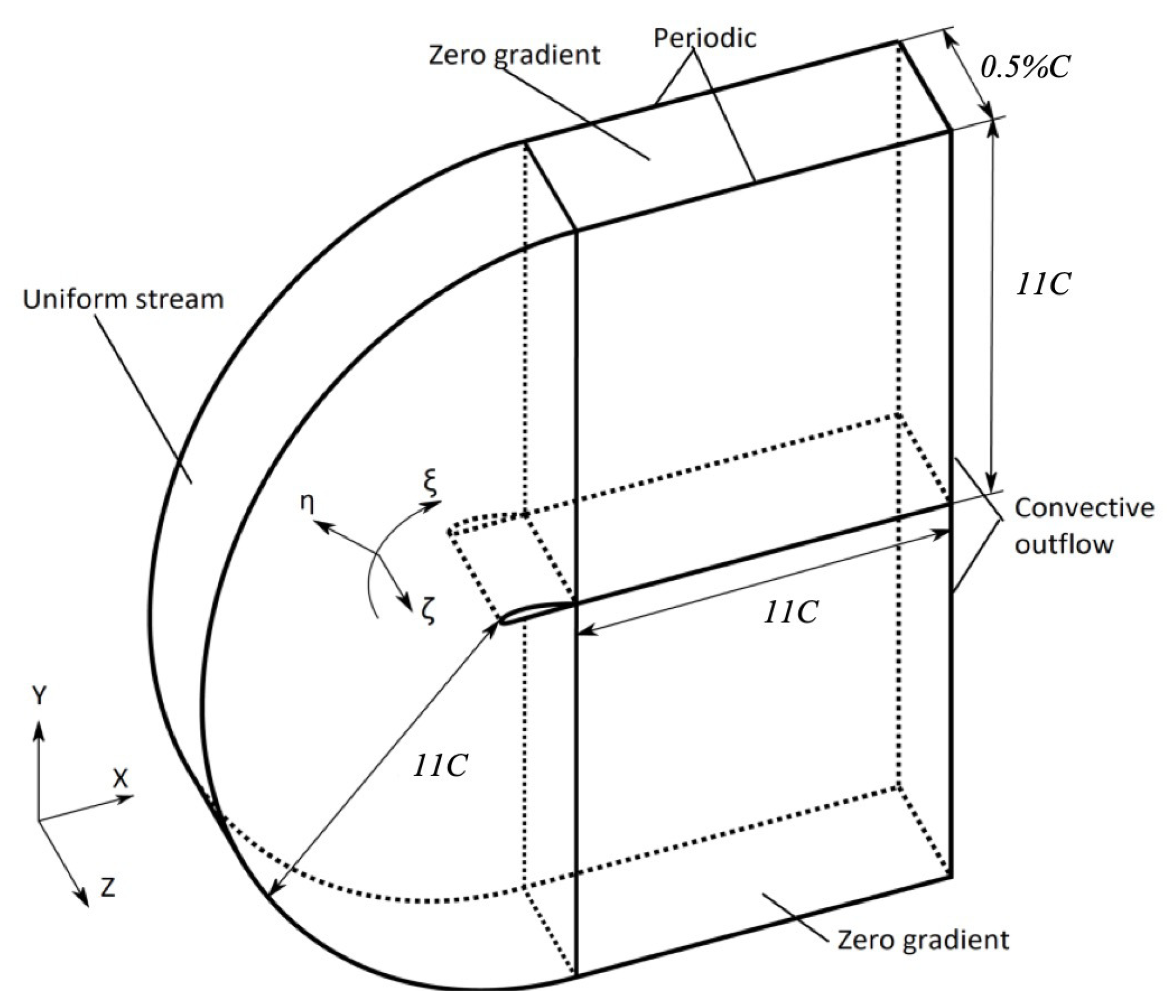
2. LES of Low Mach Number Turbulent Flows around NACA0012 Airfoil

2.1. Basic Equations and Smagorinsky Subgrid Scale (SGS) Model

The Favre-averaged filter and spatial filter are expressed as $\overline{\left(\right)}$ and $\widehat{\left(\right)}$ respectively, and are used for the continuity and Navier–Stokes equations, which include the continuity equation, momentum equations, and equation of state. In Equation (2), the eddy viscosity assumption is used for SGS turbulence stress. A non-dimensionalization is applied to all variables by means of the streamwise velocity $U_0$ and chord length C. Since the boundary-fitted-grid is employed in our computation, general curvilinear coordinates have to be applied and is represented as $\xi$, $\eta$, and $\varsigma$. Thus,

$$\frac{\partial \widehat{\rho }}{\partial t}+\frac{1}{J}\frac{\partial }{\partial {\xi }^k}\left(J\widehat{\rho }{\overline{U}}^k\right)=0,$$

(1)

$$\frac{\partial \left(\widehat{\rho }{\overline{u}}_i\right)}{\partial t}+\frac{1}{J}\frac{\partial }{\partial {\xi }^k}\left(J\widehat{\rho }{\overline{u}}_i{\overline{U}}^k\right)=-\frac{1}{J}\frac{\partial }{\partial {\xi }^k}\left[J\frac{\partial {\xi }^k}{\partial x_i}\left(\widehat{p}+\frac{2}{3}\widehat{\rho }{k}_{sgs}\right)\right]+\frac{1}{J}\frac{\partial }{\partial {\xi }^k}\left(J\frac{\partial {\xi }^k}{\partial x_i}{\sigma }_{ij}\right),$$

(2)

$$\widehat{p}=\widehat{\rho }RT,$$

(3)

where

$${\sigma }_{ij}=2\left(\frac{1}{Re}+\widehat{\rho }{\nu }_{sgs}\right)\left({\overline{S}}_{ij}-\frac{1}{3}{\delta }_{ij}{\overline{S}}_{kk}\right),$$

(4)

where J represents the Jacobian of the coordinate transformation, $\rho$ denotes the density, ${\widehat{U}}^k$ means the contravariant velocity, $k_{sgs}$ is the SGS kinetic energy, ${\delta }_{ij}$ is the Kronecker symbol, T is the absolute temperature, R is the ideal gas constant, $Re$ means the Reynolds number, as in ${\rho }_0{U}_0/\nu$, ${\overline{S}}_{ij}$ denotes the strain rate tensor

$${\overline{S}}_{ij}=\frac{1}{2}\left(\frac{\partial {\xi }^k}{\partial x_i}\frac{\partial {\overline{u}}_j}{\partial {\xi }^k}+\frac{\partial {\xi }^k}{\partial x_j}\frac{\partial {\overline{u}}_i}{\partial {\xi }^k}\right),$$

(5)

and ${\nu }_{sgs}$ means the eddy viscosity since the effect of SGS turbulence on the large-scale motion is expected to be estimated by an SGS model.

Using the local equilibrium assumption, i.e., that the dissipation rate of SGS energy is in balance with the production rate, the dynamic Smagorinsky model can be obtained for LES:

$${\nu }_{sgs}=C{\widehat{\mathsf{\Delta }}}^2\left|\overline{S}\right|,$$

(6)

in which $|\overline{S}|$ denotes the norm of the strain rate tensor and is defined as $\sqrt{2{\overline{S}}_{ij}{\overline{S}}_{ij}}$; C is a variable to be dynamically determined from the grid-scale velocity field $\overline{u}$.

Applying the test filter on the grid-filtered N-S equations, the Germano identity can be defined as

$$L_{ij}=T_{ij}-{\tilde{\tau }}_{ij}=\widetilde{{\overline{u}}_i{\overline{u}}_j}-{\tilde{\overline{u}}}_i{\tilde{\overline{u}}}_j,$$

(7)

where $L_{ij}$ can be calculated based on the resolved scales, and $T_{ij}=\widetilde{\overline{u_i{u}_j}}-\widetilde{{\overline{u}}_i}\widetilde{{\overline{u}}_j}$ represents the residual turbulent stress at a test-filter scale $\tilde{\mathsf{\Delta }}$ and can be given as

$$T_{ij}-\frac{1}{3}{\delta }_{ij}{T}_{kk}=-2C{\tilde{\mathsf{\Delta }}}^2\left|\tilde{\overline{S}}\right|{\tilde{\overline{S}}}_{ij}.$$

(8)

Upon substituting Equations (4) and (8) into Equation (7) and assuming $\widehat{\mathsf{\Delta }}$ and C are constant inside the test filter, an equation for determining C was obtained:

$$L_{ij}-\frac{1}{3}{\delta }_{ij}{L}_{kk}=-2C{\widehat{\mathsf{\Delta }}}^2{M}_{ij},$$

(9)

where

$$M_{ij}=\frac{{\tilde{\mathsf{\Delta }}}^2}{{\widehat{\mathsf{\Delta }}}^2}\left|\tilde{\overline{S}}\right|{\tilde{\overline{S}}}_{ij}-\widetilde{|\overline{S}|{\overline{S}}_{ij}}.$$

(10)

Minimization of the error of Equation (9) over all independent tensor components [29], and over some averaging region of statistical homogeneity, leads to

$$C=-\frac{1}{2{\widehat{\mathsf{\Delta }}}^2}\frac{〈L_{ij}{M}_{ij}〉}{〈M_{ij}{M}_{ij}〉}.$$

(11)

Finally, substituting the dynamically determined variable C of Equation (11) into Equation (6), the eddy viscosity ${\nu }_{sgs}$ can be computed.

Through using the CIP-combined unified numerical procedure method [30], the fractional step method is applied for time-marching of Equation (2):

$${\left(\widehat{\rho }\overline{\mathit{u}}\right)}^F=\frac{\mathsf{\Delta }t}{2}\left(\frac{2}{\mathsf{\Delta }t}{\left(\widehat{\rho }\overline{\mathit{u}}\right)}^n+3\mathsf{\nabla }·{[-\left(\widehat{\rho }\overline{\mathit{u}}\overline{\mathit{u}}\right)+\tau ]}^n-\mathsf{\nabla }·{[-\left(\widehat{\rho }\overline{\mathit{u}}\overline{\mathit{u}}\right)+\tau ]}^{n-1}\right),$$

(12)

$${\left(\widehat{\rho }\overline{\mathit{u}}\right)}^{n+1}={\left(\widehat{\rho }\overline{\mathit{u}}\right)}^F-\mathsf{\Delta }t\mathsf{\nabla }{\widehat{p}}^{n+1},$$

(13)

in which $\tau$ represents the viscous stress, $\mathsf{\Delta }t$ the time increment, and n the time step count. The advancement method of time for Equation (1) can be written as:

$${\widehat{\rho }}^{n+1}={\widehat{\rho }}^n-\mathsf{\Delta }t\mathsf{\nabla }·{\left(\widehat{\rho }\overline{\mathit{u}}\right)}^{n+1}.$$

(14)

Applying the divergence for Equation (13) and then substitution of this divergence into Equation (14) leads to the pressure elliptic equation for ${\widehat{p}}^{n+1}$.

$$-{\widehat{\rho }}^{n+1}+{\widehat{\rho }}^n-\mathsf{\Delta }t\mathsf{\nabla }·{\left(\widehat{\rho }\overline{\mathit{u}}\right)}^F=-\mathsf{\Delta }{t}^2{\mathsf{\nabla }}^2{\widehat{p}}^{n+1}.$$

(15)

In order to take the compressibility into account for the pressure equation, Equation (3) can be written as the following for weakly compressible flows:

$${\widehat{p}}^{n+1}-{\widehat{p}}^n=({\widehat{\rho }}^{n+1}-{\widehat{\rho }}^n)RT.$$

(16)

Substituting Equation (16) into Equation (15) results in a pressure equation that accounts for the compressibility; thus,

$${\left(\mathsf{\Delta }t\right)}^{2}RT{\mathsf{\nabla }}^2{\widehat{p}}^{n+1}-{\widehat{p}}^{n+1}=\left(\mathsf{\Delta }t\right)RT\mathsf{\nabla }·{\left(\widehat{\rho }\overline{\mathit{u}}\right)}^F-{\widehat{p}}^n.$$

(17)

Therefore, the second term in two sides of Equation (17) accounts for the compressibility effect. In a word, using Equation (17), ${\widehat{p}}^{n+1}$ is solved; and then, substituting ${\widehat{p}}^{n+1}$ into Equation (12), ${\left(\widehat{\rho }\overline{\mathit{u}}\right)}^{n+1}$ is calculated; and finally, applying (1), ${\widehat{\rho }}^{n+1}$ is obtained. Note that he applicability of this procedure is limited with weakly compressible flows due to the fact that $\mathsf{\Delta }\widehat{p}$ and $\mathsf{\Delta }\widehat{\rho }$ change very slightly in one time step for the low Mach number turbulent flow.

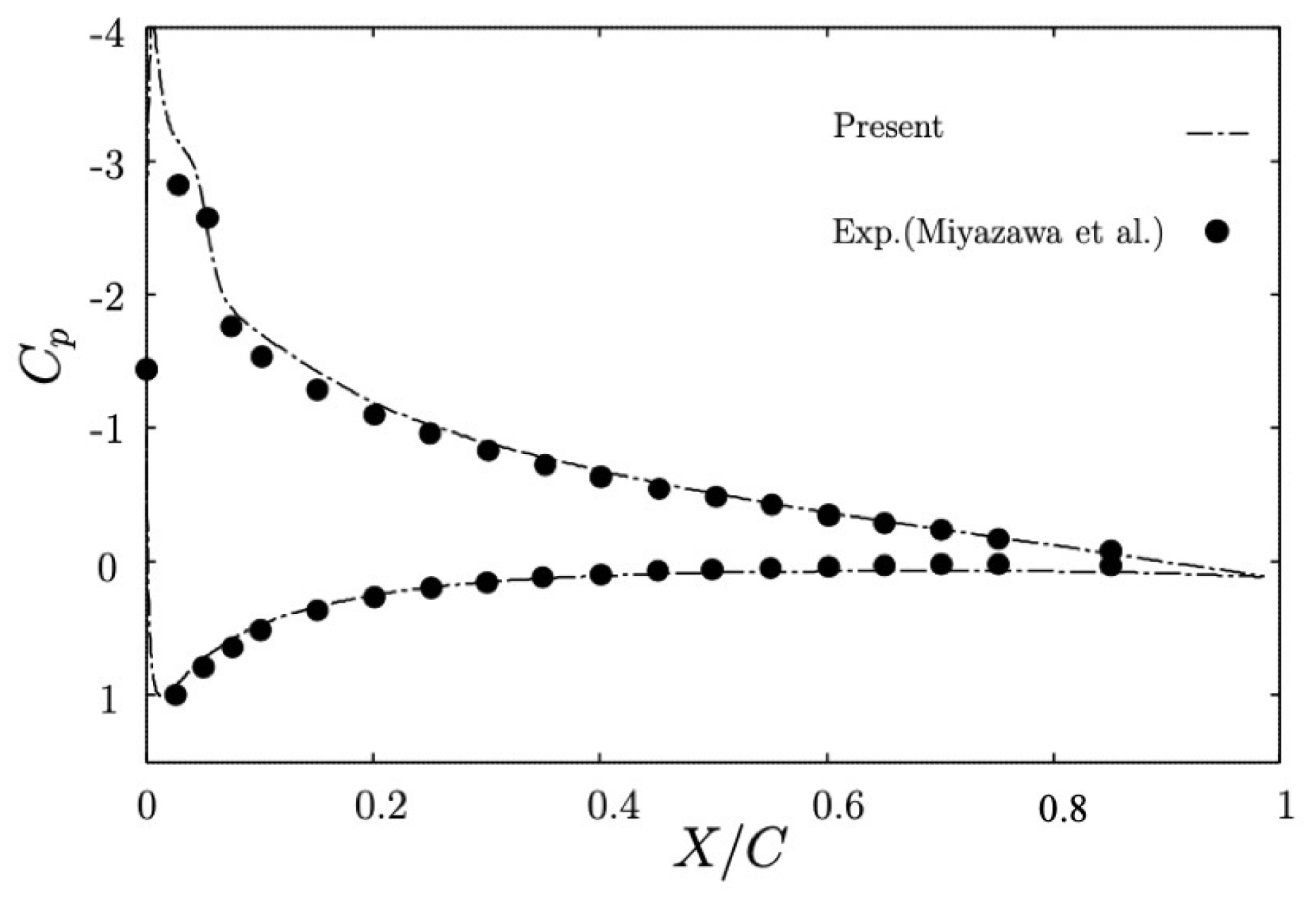
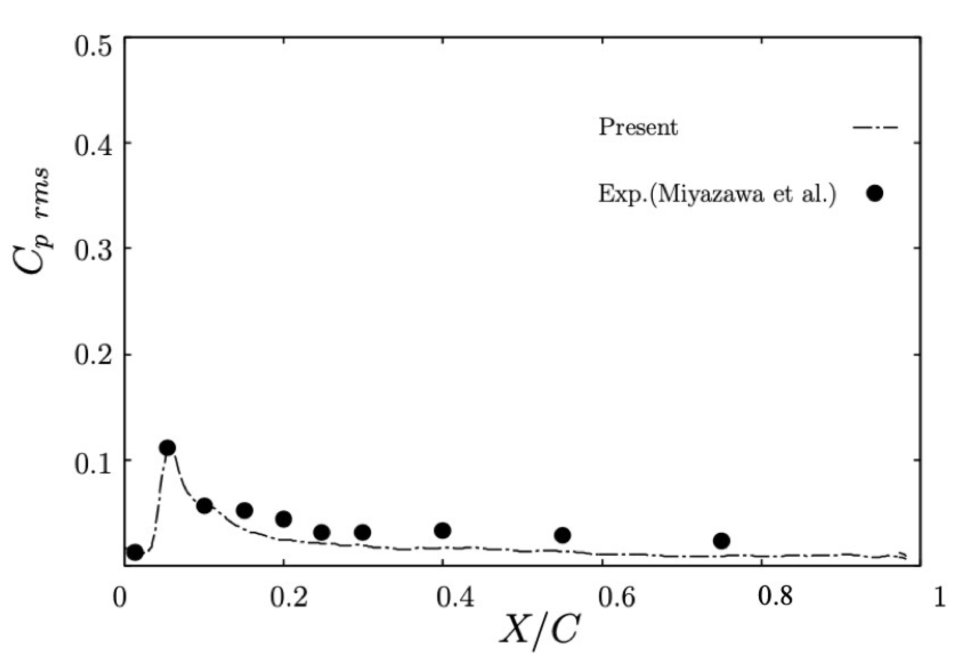
2.2. Validation of LES for Low Mach Number Turbulent Flows around NACA0012 Airfoil

The calculation target of this study is a three-dimensional flow around a two-dimensional wing of the NACA0012 airfoil, which is a typical streamlined object. NACA0012 airfoil is defined by the following equation and its geometry is given in Figure 1.

$$\pm y/C=0.6\times \left[0.2969\sqrt{x/C}-0.1260(x/C)-0.3516{(x/C)}^2+0.2843{(x/C)}^3-0.01015{(x/C)}^4\right].$$

(18)

In order to validate our method, we conducted a LES of the compressible flow around NACA0012 airfoil with the computational setup matching the experimental setup of Miyazawa et al. [31], in which the Mach number was $8.75\times {10}^{-2}$, the angel of attack was $9^{\circ }$, and the Reynolds number was $2\times {10}^5$, which was based on the uniform velocity in the streamwise direction and the chord length. Figure 2 shows the computational domain and computational boundary conditions in the present study. For the Cartesian coordinate system, x, z, and y were defined in the streamwise direction, spanwise direction, and vertical direction, respectively. We used a C-type boundary-fitted grid in the x–y plane. Thus, a general curvilinear coordinate system had to be applied and represented as $\xi$, $\eta$, $\zeta$ for all computations, in which the direction following the mainstream surface of the airfoil is denoted as $\xi$, the direction away from the surface of airfoil is defined as $\eta$, and the spanwise direction is represented as $\zeta$. The computational domain size is defined as the following: the length of the wake, the semidiameter of the C-type grid, and the spanwise extent were $11C$, $11C$, and $0.5\%C$, respectively. Here, C is chord length. For the mesh, there were 1600 grid points in the $\xi$ direction, in which 800 was on the airfoil surface, 160 grid points were in the $\eta$ direction, and 60 grid points were in the $\zeta$ direction. As shown in Figure 2, the non-slip boundary condition was applied on the airfoil surface. The inflow was the uniform stream without disturbance. The convective outflow was applied for the outflow boundary condition. The spanwise direction boundary condition is defined as the periodic. For the variables in the $\eta$ direction, zero gradient was employed at the op and bottom boundary. Particular attention was paid for the non-reflective boundary condition by [32] at the far boundary.

A second-order central finite-difference discretization scheme was applied in the equation of motion for the diffusion terms. In order to improve the numerical stability in high Reynolds number flow, a QUICK method was applied for the convective terms in the general curvilinear coordinate system. For coupling the pressure field and the continuity equation, the fractional method was applied. The second-order Adams–Bashforth method is used to the convective term and the viscous term for the advancement method of time in the equation of motion. For the dynamic procedure, the test filter was used in the streamwise direction and spanwise direction with second-order accuracy and the test-to-grid filter ratio $\tilde{\mathsf{\Delta }}/\widehat{\mathsf{\Delta }}=2$. The present numerical method and computer program have been tested extensively in several turbulent flows [33,34,35,36,37].

All simulations were computed on an NEC SX-8R supercomputer of Cybermedia Center, Osaka University with the time step $dt=0.0495H/U_c$. The greater part of the total effort toward calculations was spent on solving the pressure equation through the residual cutting method [38]. All simulations were run until the flow fields that were fully developed and the first-order, and second-order statistics exhibited adequate convergence. The time-averaging, and, the spatial averaging in the spanwise direction were used for collecting the data. Figure 3 and Figure 4 show the distribution of the mean pressure coefficient $C_p$ on the airfoil surface and the average pressure coefficient fluctuation $C_{prms}$ on the suction side of the airfoil, in which $C_p$ is defined by the freestream pressure $p_0$.

$$C_p=\frac{p-p_0}{\frac{1}{2}\rho U_0^2}.$$

(19)

Then, the root-mean-square of $C_p$ is defined as $C_{prms}$. In order to demonstrate the validity of our model, the results of our LES are compared with the measurement by [31]. In Figure 3 and Figure 4, our computational results are in good agreement with the experimental data.

3. Derivation of a New Acoustic Model

A new acoustic model was derived by using the compressible continuity and Navier–Stokes equations of the flow field; i.e.,

$$\frac{\partial \rho }{\partial t}+\frac{1}{J}\frac{\partial }{\partial {\xi }^k}\left(J\frac{\partial {\xi }^k}{\partial x_i}\rho u_j\right)=0,$$

(20)

$$\frac{\partial u_i}{\partial t}+\frac{1}{J}\frac{\partial }{\partial {\xi }^k}\left(J\frac{\partial {\xi }^k}{\partial x_j}\rho u_j{u}_i\right)-\frac{\partial {\xi }^k}{\partial x_i}\frac{\partial p}{\partial {\xi }^k}=\frac{\partial {\xi }^k}{\partial x_j}\frac{\partial {\sigma }_{ij}}{\partial {\xi }^k},$$

(21)

$${\sigma }_{ij}=2\mu \left(S_{ij}-\frac{1}{3}{\delta }_{ij}{S}_{kk}\right),S_{ij}=\frac{1}{2}\left(\frac{\partial {\xi }^k}{\partial x_i}\frac{\partial u_j}{\partial {\xi }^k}+\frac{\partial {\xi }^k}{\partial x_j}\frac{\partial u_i}{\partial {\xi }^k}\right).$$

(22)

Variables $\rho$ and p are decomposed as

$$\rho ={\rho }_0+{\rho }^{\prime },p=p_0+p^{\prime },$$

(23)

where (0) indicates the mean component of variables; (${}^{\prime }$) means the perturbation component of variables, due to in low Mach number turbulent flow

$${\rho }_0\gg {\rho }^{\prime },p_0\gg p^{\prime }.$$

(24)

Rewriting Equations (20) and (21) by using Equation (23) leads to

$$\frac{\partial {\rho }^{\prime }}{\partial t}+\frac{1}{J}\frac{\partial }{\partial {\xi }^k}\left(J\frac{\partial {\xi }^k}{\partial x_i}{\rho }^{\prime }{u}_j\right)=-{\rho }_0\frac{\partial {\xi }^k}{\partial x_j}\frac{\partial u_j}{\partial {\xi }^k},$$

(25)

$$\frac{\partial u_i}{\partial t}+\frac{1}{J}\frac{\partial }{\partial {\xi }^k}\left(J\frac{\partial {\xi }^k}{\partial x_j}{u}_j{u}_i\right)-\frac{1}{\rho }\frac{\partial {\xi }^k}{\partial x_i}\frac{\partial p^{\prime }}{\partial {\xi }^k}=\frac{1}{\rho }\frac{\partial {\xi }^k}{\partial x_j}\frac{\partial {\sigma }_{ij}}{\partial {\xi }^k}.$$

(26)

After multiplying $u_i$ to Equation (25) and ${\rho }^{\prime }$ to Equation (26), Equations (25) and (26) are added. Namely,

$$\frac{\partial {\rho }^{\prime }{u}_i}{\partial t}+\frac{1}{J}\frac{\partial }{\partial {\xi }^k}\left(J\frac{\partial {\xi }^k}{\partial x_i}{\rho }^{\prime }{u}_i{u}_j\right)+\frac{{\rho }^{\prime }}{\rho }\frac{\partial {\xi }^k}{\partial x_i}\frac{\partial p^{\prime }}{\partial {\xi }^k}=\frac{{\rho }^{\prime }}{\rho }\frac{\partial {\xi }^k}{\partial x_j}\frac{\partial {\sigma }_{ij}}{\partial {\xi }^k}-{\rho }_0{u}_i\frac{\partial {\xi }^k}{\partial x_j}\frac{\partial u_j}{\partial {\xi }^k}.$$

(27)

Taking the divergence of Equation (27), subtracting $\frac{\partial }{\partial t}$ of Equation (25), and then adding $-c_0^2\frac{1}{J}\frac{\partial }{\partial {\xi }^k}\left({\gamma }^{kl}\frac{\partial {\rho }^{\prime }}{\partial {\xi }^l}\right)$ concerning two sides of the equation obtained, the wave equation with source terms is finally obtained as the following

$$\begin{array}{cc} & \frac{{\partial }^2{\rho }^{\prime }}{\partial t^2}-c_0^2\frac{1}{J}\frac{\partial }{\partial {\xi }^k}\left({\gamma }^{kl}\frac{\partial {\rho }^{\prime }}{\partial {\xi }^l}\right)=\frac{1}{J}\frac{\partial }{\partial {\xi }^k}\left({\gamma }^{kl}\frac{\partial }{\partial {\xi }^l}{\rho }^{\prime }{u}_i{u}_j\right)-c_0^2\frac{1}{J}\frac{\partial }{\partial {\xi }^k}\left({\gamma }^{kl}\frac{\partial {\rho }^{\prime }}{\partial {\xi }^l}\right)\hfill \\ +& \frac{{\rho }^{\prime }}{\rho }\frac{1}{J}\frac{\partial }{\partial {\xi }^k}\left({\gamma }^{kl}\frac{\partial {\rho }^{\prime }}{\partial {\xi }^l}\right)+\frac{\partial {\xi }^l}{\partial x_i}\frac{\partial p^{\prime }}{\partial {\xi }^l}\frac{\partial {\xi }^k}{\partial x_i}\frac{\partial }{\partial {\xi }^k}\frac{{\rho }^{\prime }}{\rho }-{\rho }_0\frac{\partial }{\partial t}\left(\frac{{\xi }^k}{\partial x_i}\frac{\partial u_i}{\partial {\xi }^k}\right)-\frac{{\rho }^{\prime }}{\rho }\frac{1}{J}\frac{\partial }{\partial {\xi }^k}\left({\gamma }^{kl}\frac{\partial }{\partial {\xi }^l}{\sigma }_{ij}\right)\hfill \\ -& \frac{\partial {\xi }^k}{\partial x_i}\frac{\partial {\xi }^l}{\partial x_j}\frac{\partial {\sigma }_{ij}}{\partial {\xi }^k}\frac{\partial }{\partial {\xi }^l}\left(\frac{{\rho }^{\prime }}{\rho }\right)+{\rho }_0\frac{\partial {\xi }^l}{\partial x_i}\frac{\partial {\xi }^k}{\partial x_j}\frac{\partial u_i}{\partial {\xi }^l}\frac{\partial u_j}{\partial {\xi }^k}+{\rho }_0{u}_i\frac{1}{J}\frac{\partial }{\partial {\xi }^k}\left({\gamma }^{kl}\frac{\partial u_j}{\partial {\xi }^l}\right).\hfill \end{array}$$

(28)

The first term and the last term of the right-hand side of Equation (29) can be rewritten as

$$\frac{1}{J}\frac{\partial }{\partial {\xi }^k}\left({\gamma }^{kl}\frac{\partial }{\partial {\xi }^l}{\rho }^{\prime }{u}_i{u}_j\right)+{\rho }_0{u}_i\frac{1}{J}\frac{\partial }{\partial {\xi }^k}\left({\gamma }^{kl}\frac{\partial u_j}{\partial {\xi }^l}\right)=\frac{1}{J}\frac{\partial }{\partial {\xi }^k}\left({\gamma }^{kl}\frac{\partial }{\partial {\xi }^l}\rho u_i{u}_j\right)+{\rho }_0{u}_j\frac{\partial {\xi }^k}{\partial x_j}\frac{\partial }{\partial {\xi }^k}\left(\frac{\partial {\xi }^l}{\partial x_i}\frac{\partial u_i}{\partial {\xi }^l}\right).$$

(29)

Upon substituting Equation (29) into Equation (29), the wave equation with a lump of source terms is obtained as follows

$$\begin{array}{ccc}\frac{{\partial }^2{\rho }^{\prime }}{\partial t^2}-c_0^2\frac{1}{J}\frac{\partial }{\partial {\xi }^k}\left({\gamma }^{kl}\frac{\partial {\rho }^{\prime }}{\partial {\xi }^l}\right)\hfill & =& \frac{1}{J}\frac{\partial }{\partial {\xi }^k}\left({\gamma }^{kl}\frac{\partial }{\partial {\xi }^l}\rho u_i{u}_j\right)-c_0^2\frac{1}{J}\frac{\partial }{\partial {\xi }^k}\left({\gamma }^{kl}\frac{\partial {\rho }^{\prime }}{\partial {\xi }^l}\right)+\frac{{\rho }^{\prime }}{\rho }\frac{1}{J}\frac{\partial }{\partial {\xi }^k}\left({\gamma }^{kl}\frac{\partial {\rho }^{\prime }}{\partial {\xi }^l}\right)\hfill \\ & +& \frac{\partial {\xi }^l}{\partial x_i}\frac{\partial p^{\prime }}{\partial {\xi }^l}\frac{\partial {\xi }^k}{\partial x_i}\frac{\partial }{\partial {\xi }^k}\frac{{\rho }^{\prime }}{\rho }-\frac{{\rho }^{\prime }}{\rho }\frac{1}{J}\frac{\partial }{\partial {\xi }^k}\left({\gamma }^{kl}\frac{\partial }{\partial {\xi }^l}{\sigma }_{ij}\right)\hfill \\ & -& \frac{\partial {\xi }^k}{\partial x_i}\frac{\partial {\xi }^l}{\partial x_j}\frac{\partial {\sigma }_{ij}}{\partial {\xi }^k}\frac{\partial }{\partial {\xi }^l}\left(\frac{{\rho }^{\prime }}{\rho }\right)-{\rho }_0\frac{D}{Dt}\left(\mathsf{\nabla }·\mathbf{u}\right)+{\rho }_0{\left(\mathsf{\nabla }·\mathbf{u}\right)}^2,\hfill \end{array}$$

(30)

where $\frac{D}{Dt}=\frac{\partial }{\partial t}+u_j\frac{\partial }{\partial x_j}$ means the material derivative. Here, assuming a low Mach number flow (${\rho }_0\gg {\rho }^{\prime }$) and a high Reynolds number flow (${\delta }_{ij}\ll 1$ ), a wave equation with source terms can be finally obtained as

$$\frac{{\partial }^2{\rho }^{\prime }}{\partial t^2}-c_0^2\frac{1}{J}\frac{\partial }{\partial {\xi }^k}\left({\gamma }^{kl}\frac{\partial {\rho }^{\prime }}{\partial {\xi }^l}\right)=\frac{1}{J}\frac{\partial }{\partial {\xi }^k}\left({\gamma }^{kl}\frac{\partial }{\partial {\xi }^l}\rho u_i{u}_j\right)-c_0^2\frac{1}{J}\frac{\partial }{\partial {\xi }^k}\left({\gamma }^{kl}\frac{\partial {\rho }^{\prime }}{\partial {\xi }^l}\right)-{\rho }_0\frac{D}{Dt}\left(\mathsf{\nabla }·\mathbf{u}\right)+{\rho }_0{\left(\mathsf{\nabla }·\mathbf{u}\right)}^2.$$

(31)

The form of our wave Equation (31) is similar to the form of the following Lighthill’s equation [11]. Lighthill’s equation is expressed as

$$\frac{{\partial }^2{\rho }^{\prime }}{\partial t^2}-c_0^2\frac{1}{J}\frac{\partial }{\partial {\xi }^k}\left({\gamma }^{kl}\frac{\partial {\rho }^{\prime }}{\partial {\xi }^l}\right)=\frac{1}{J}\frac{\partial }{\partial {\xi }^k}\left({\gamma }^{kl}\frac{\partial T_{ij}}{\partial {\xi }^l}\right),$$

(32)

where

$$T_{ij}=\rho u_i{u}_j+{\delta }_{ij}\left[(p-p_0)-c_0^2(\rho -{\rho }_0)\right]-{\sigma }_{ij}.$$

(33)

Equation (31) and Lighthill’s Equation (32) both seem to be wave equations having the source terms on the right hand side. But there are unknowns in $T_{ij}$ for Lighthill’s Equation (32). Especially in case of low Mach number flows, the simplification of $T_{ij}\approx {\rho }_0{u}_i{u}_j$ works well. Hence the indirect method, which solves the acoustic field using $T_{ij}$ given by the incompressible solver, becomes reasonable. On the other hand, from our wave Equation (31), the utilization of $\mathsf{\nabla }·\mathbf{u}$ for the sound source is possible. Actually, the divergence of the velocity vector plays an important role in the flow field even in the low Mach number [34]. Therefore, we rearranged the acoustic wave equation by exposing $\mathsf{\nabla }·\mathbf{u}$ intentionally and then obtained Equation (31), so that the indirect method could be extended from the zero Mach number region to low or moderate Mach number region.

For easily applying to engineering practices in the industry, such as large-scale wind turbine blades and underlining the key role of $\mathsf{\nabla }·\mathbf{u}$ in the flow field, our acoustic model Equation (31) can be further approximated as

$$\frac{{\partial }^2{\rho }^{\prime }}{\partial t^2}-c_0^2\frac{1}{J}\frac{\partial }{\partial {\xi }^k}\left({\gamma }^{kl}\frac{\partial {\rho }^{\prime }}{\partial {\xi }^l}\right)\approx -{\rho }_0\frac{D}{Dt}\left(\mathsf{\nabla }·\mathbf{u}\right)+{\rho }_0{\left(\mathsf{\nabla }·\mathbf{u}\right)}^2.$$

(34)

The Lighthill’s Equation (32) is exact, but some kind of turbulence modeling for computing the sound source is required when the Reynolds number is high. Especially in case of low Mach number flows, the simplification of $T_{ij}\approx {\rho }_0{u}_i{u}_j$ is utilized so that the solver becomes incompressible. Powell’s sound source model [19] is derived under the assumption of incompressible flows. On the other hand, although some approximation is used in the derivation of the acoustic equation, our sound source model (34) does not need any modeling process. Furthermore, it can consider the influence of the compressibility effect. Thus, the behavior of sound source due to the variation of Mach number is expected to be reproduced appropriately.

Applying our acoustic theory and the compact green function [22], the sound pressure in the far-field is solved from the wave Equation (34). That is, assuming that the observation point x is sufficiently far from the sound source area of the objet y, the object keep stationary and the velocity of the surface S of the object is zero, the wave Equation (34) is able to be solved applying the compact green function:

$$p_a(\mathit{x},t)={\rho }_0\int \int \frac{D}{Dt}(\mathsf{\nabla }·\mathbf{u})·\mathsf{\nabla }G(\mathit{x},\mathit{y},t-\mathit{\tau })d^3\mathit{y}d\mathit{\tau },$$

(35)

where $p_a$ denotes the pressure sound, G means the compact green function and is represented as

$$G(\mathit{x},\mathit{y},t-\mathit{\tau })=\frac{1}{4\pi \left|\mathit{x}\right|}\delta \left(t-\mathit{\tau }\frac{\left|\mathit{x}\right|}{c_0}\right)+\frac{\mathit{x}·\mathit{Y}}{4\pi c_0{\left|\mathit{x}\right|}^2}\frac{\partial }{\partial t}\delta \left(t-\mathit{\tau }-\frac{\left|\mathit{x}\right|}{c_0}\right).$$

(36)

Here, $\mathit{Y}$ means Kirchhoff vector and is calculated through ${\mathsf{\nabla }}^2{\mathit{Y}}_i=0$. Then substitution of Equation (36) into Equation (35) results in

$$p_a^{\prime }(\mathit{x},t)=\frac{{\rho }_0{x}_i}{4\pi c_0{\left|\mathit{x}\right|}^2}\frac{\partial }{\partial t}\int \frac{D}{Dt}(\mathsf{\nabla }·\mathbf{u})\left(\mathit{y},t-\frac{\left|\mathit{x}\right|}{c_0}\right)\mathsf{\nabla }{\mathit{Y}}_i\left(\mathit{y}\right)d^3\mathit{y}.$$

(37)

From the Equation (37), the sound pressure $p_a^{\prime }$ can be obtained from conducting the Fourier transform. Finally the sound pressure level (SPL) can be calculated from the following equation through applying the solved $p_a^{\prime }$:

$$SPL\left(dB\right)=10\times log\left(\frac{{p^{\prime }}_a^2}{P_b^2}\right),$$

(38)

where $P_b$ means the reference sound pressure. In general, the magnitude of $P_b$ is $P_b=2\times {10}^{-5}Pa$.

4. Results of the Acoustic Field around NACA0012 Airfoil

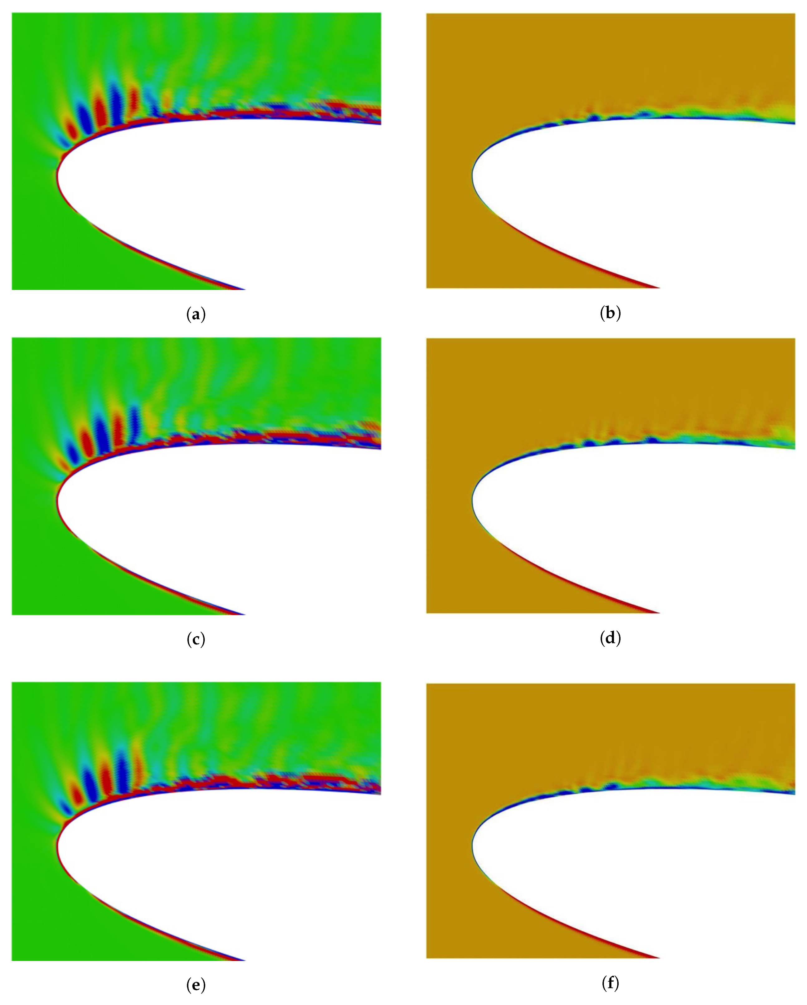
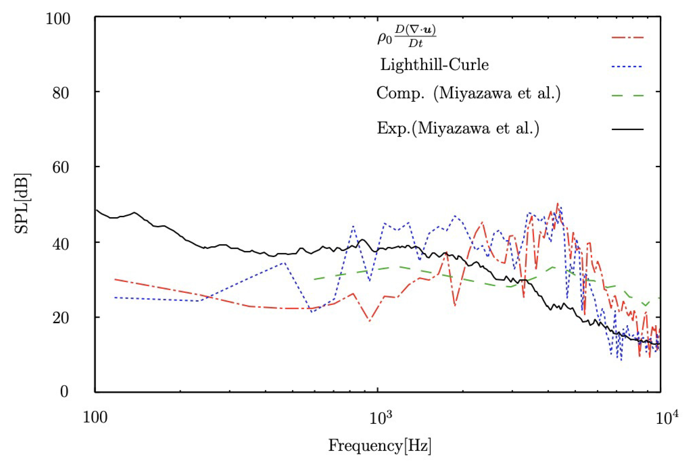
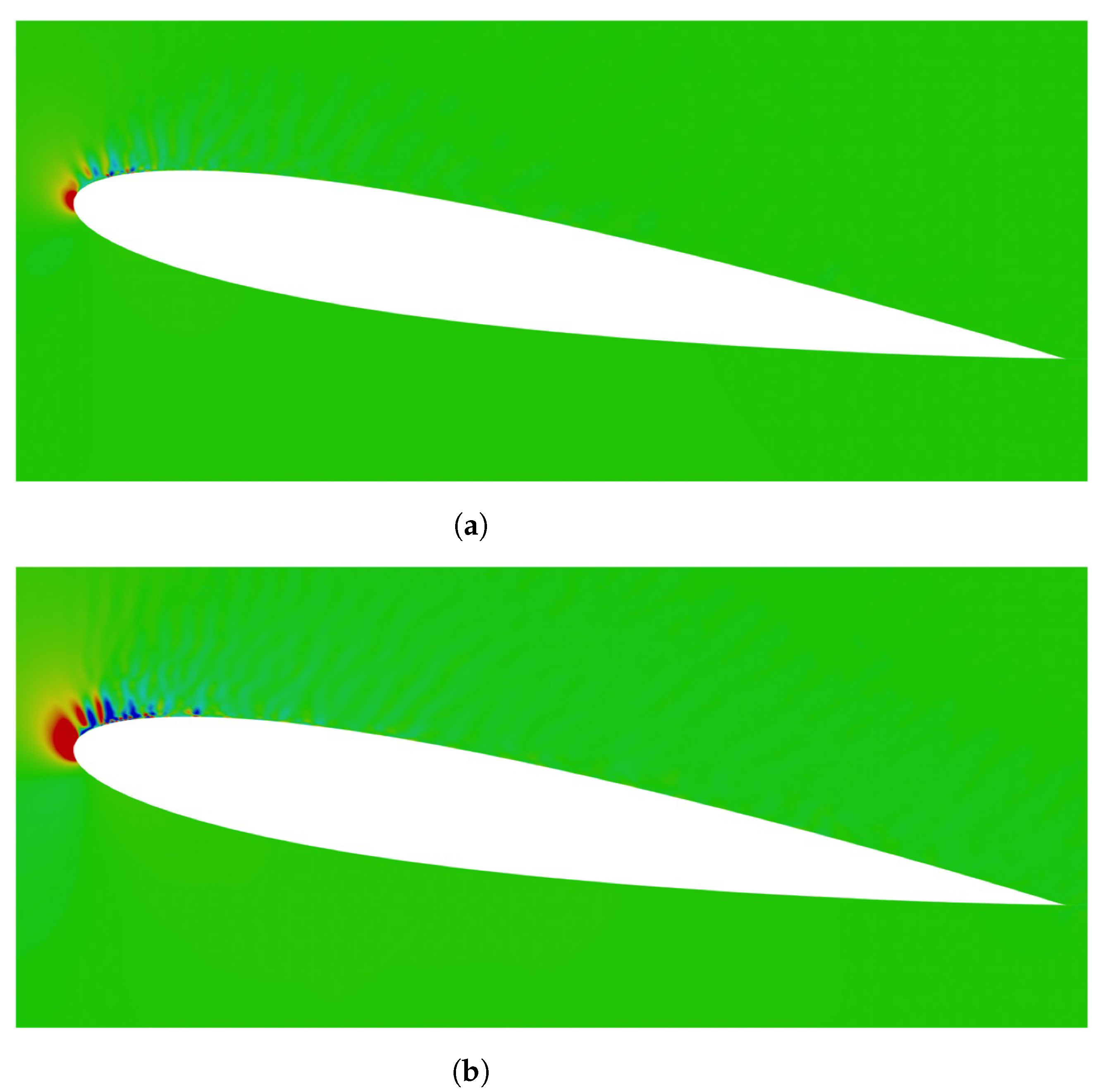
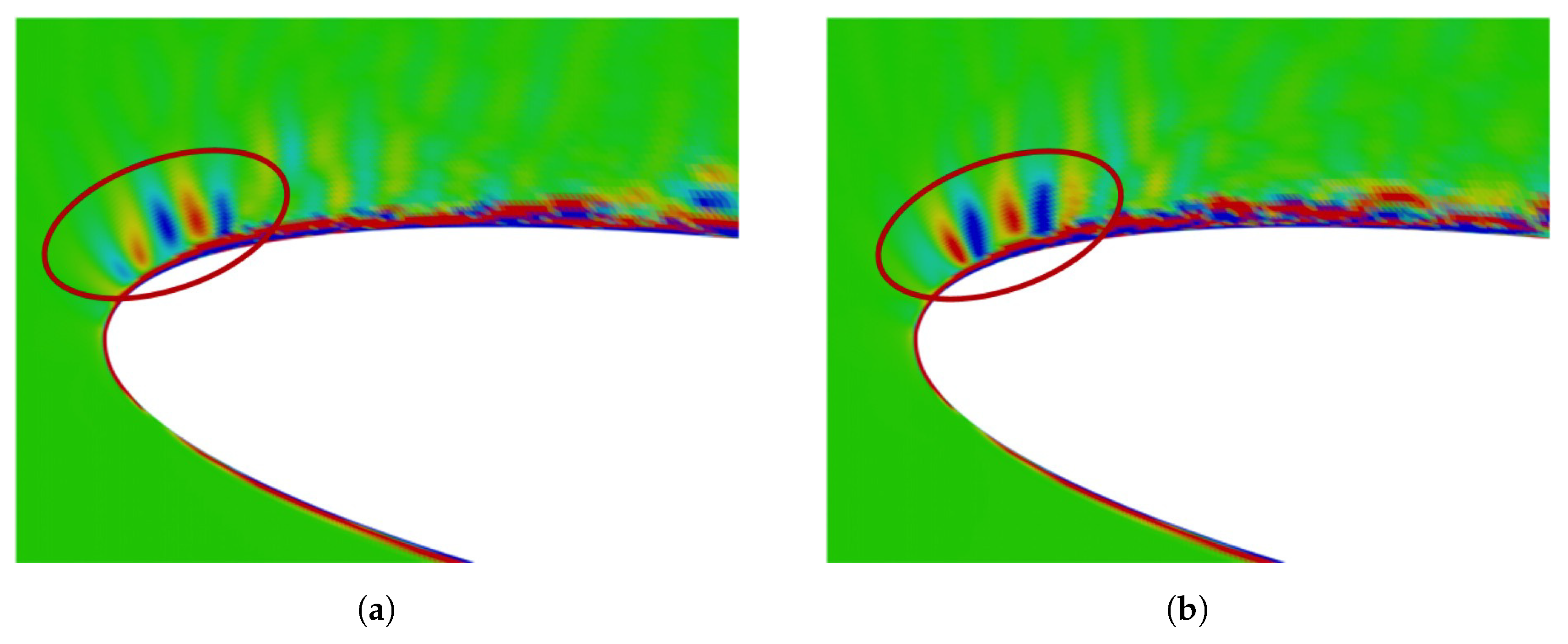
4.1. Comparison of Different Sound Source Detection

In this section, using LES databases obtained in Section 2 for the weakly compressible flow field around NACA0012 airfoil under the conditions of $Re=2\times {10}^5$, $M=0.0875$, and $\alpha =9^{\circ }$, results of the sound field due to the flow field are discussed. The relationship between our proposed sound source model (34) and the classical sound source models by Lighthill [11] and Powell [19] is discussed through the comparison of the distribution of sound source terms around the airfoil using our LES database, as shown in Figure 5. Figure 5a,b show the instantaneous and cross-sectional profiles of the well-know classical sound source models of $\mathsf{\nabla }·(\mathsf{\nabla }·\mathbf{T})$ by Lighthill [11] and $\mathsf{\nabla }·(\omega \times \mathit{u})$ by Powell [19], respectively; Figure 5c,d show the instantaneous and cross-sectional profiles of our derived sound source of Equation (34) for $-{\rho }_0\frac{D}{Dt}(\mathsf{\nabla }·\mathbf{u})$ and ${\rho }_0{(\mathsf{\nabla }·\mathbf{u})}^2$, respectively. Because the experimentally estimated sound source which was caused by the separation bubble was confirmed near the leading-edge, we focused on that region. In Figure 5a–c, the distributions of $\mathsf{\nabla }·(\mathsf{\nabla }·\mathbf{T})$, $\mathsf{\nabla }·(\omega \times \mathit{u})$, and $-{\rho }_0\frac{D}{Dt}(\mathsf{\nabla }·\mathbf{u})$ are locally similar, near the leading edge. Pairs of positive and negative patterns are observed near the leading edge in the suction side, and intense regions correspond to the experimentally estimated sound source region. But, the distribution of ${\rho }_0{(\mathsf{\nabla }·\mathbf{u})}^2$ differs from the other terms and has a relatively very small value. Therefore, from Figure 5, it is considered that ${\rho }_0{(\mathsf{\nabla }·\mathbf{u})}^2$ does not nearly contribute to the sound field, while ${\rho }_{\infty }\frac{D}{Dt}(\mathsf{\nabla }·\mathbf{u})$ plays an important role in generation of sound.

According to the theory of vortex sound by Powell [19] and Howe [22], the main sound source of the aerodynamic noise is related to the behavior of vortex. Thus, the comparison of the behavior of the spanwise vorticity ${\omega }_z$ and the main sound source $-{\rho }_0\frac{D}{Dt}(\mathsf{\nabla }·\mathbf{u})$ was conducted. Figure 6 shows time evolution of instantaneous and cross-sectional profiles of $-{\rho }_0\frac{D}{Dt}(\mathsf{\nabla }·\mathbf{u})$ and ${\omega }_z$ near the leading edge. The significant distribution of ${\omega }_z$ exists in the suction side, and its region is similar to the distribution region of $-{\rho }_0\frac{D}{Dt}(\mathsf{\nabla }·\mathbf{u})$, apart from the area of strong compressibility. Moreover, the period of moving of $-{\rho }_0\frac{D}{Dt}(\mathsf{\nabla }·\mathbf{u})$ corresponds to that of ${\omega }_z$: its value is $2.3\times {10}^{-4}$. From results that time evolution of $-{\rho }_0\frac{D}{Dt}(\mathsf{\nabla }·\mathbf{u})$ is similar to the time evolution of the unsteady vortex ${\omega }_z$ near the leading edge, and the distribution of $-{\rho }_0\frac{D}{Dt}(\mathsf{\nabla }·\mathbf{u})$ is similar to the distribution of ${\rho }_0\mathsf{\nabla }·(\omega \times \mathit{u})$, it is considered that our sound source model might reproduce the vortex sound appropriately.

We compared sound pressure levels (SPL) for different acoustic models using our LES database and the published results from computation and measurement in the far-field; see Figure 7. The sound pressure in the far-field for our acoustic model was obtained by Equation (37) and converted to SPL by Equation (38). It is necessary to perform volume integration when determining the sound pressure in our sound source model. And the range of volume integration is determined by reference to the distribution of ${\rho }_0\mathsf{\nabla }·\left[(\mathit{u}·\mathsf{\nabla })\mathit{u}\right]$ in Figure 5 and in consideration of the calculation costs. In Figure 7, the SPL profile calculated from the Lighthill–Curle’s equation [18] employing our LES database was computed through following equation

$$p_a^{\prime }(\mathit{x},t)=\frac{{\rho }_0{x}_i}{4\pi c_0{\left|\mathit{x}\right|}^2}\frac{\partial }{\partial t}\int n_j{p}^{\prime }{\delta }_{ij}\left(\mathit{y},t-\frac{\left|\mathit{x}\right|}{c_0}\right)\mathsf{\nabla }{\mathit{Y}}_i\left(\mathit{y}\right)d^3\mathit{y},$$

(39)

where $p^{\prime }$ is the sound pressure, $\mathbf{x}$ the observation point, $\mathbf{y}$ the sound source point, $n_j$ the component of the outward pointing unit normal of the surface, and $c_0$ the speed of sound. Finally, the SPL is converted by Equation (38). In order to correspond to the experimental conditions of Miyazawa et al. [31] in the prediction of sound pressure, for the computed SPL, the representative velocity in the main flow direction is set to $U_0=30\times m/s$, the chord length is $C=0.1m$, and the observation point is $1m$ away from the leading edge in the direction normal to the streamwise direction.

Overall, the SPL profiles by $-{\rho }_0\frac{D}{Dt}(\mathsf{\nabla }·\mathbf{u})$ and the Lighthill–Curle’s method obtained by our LES do not agree well with the experimental data. However, the SPL profile obtained by the calculation of Miyazawa et al. [31] does not agree with their experimental data either. The reason for the discrepancies between the experimental data and the results obtained by the numerical calculations may be lack of resolution in the simulation of the flow field, or the compact assumption that the sound source area is regarded as a point source in sound pressure prediction. Thus to verify our sound source model, we focused on comparing the SPL profile calculated from the Lighthill–Curle’s method which is widely used for sound pressure prediction, and the SPL profile obtained by our sound source model $-{\rho }_0\frac{D}{Dt}(\mathsf{\nabla }·\mathbf{u})$. Both SPL profiles were in reasonable agreement, especially in high-frequency regions. On the other hand, in both cases, the peak value existed at about 4300 Hz. This frequency is in good agreement with the period of the moving of positive and negative patterns near the leading edge in the suction side confirmed in Figure 5c. The computational cost to use $-{\rho }_0\frac{D}{Dt}(\mathsf{\nabla }·\mathbf{u})$ as a sound source increases approximately $40\%$ against the Lighthill–Curle analogy, due to the volume integral required in our method, while the Lighthill–Curle formulation needs only surface integral. But our method enables the understanding of the relationship between the behavior of the sound source and the sound generation. Moreover, our method might be applicable to higher Mach numbers.

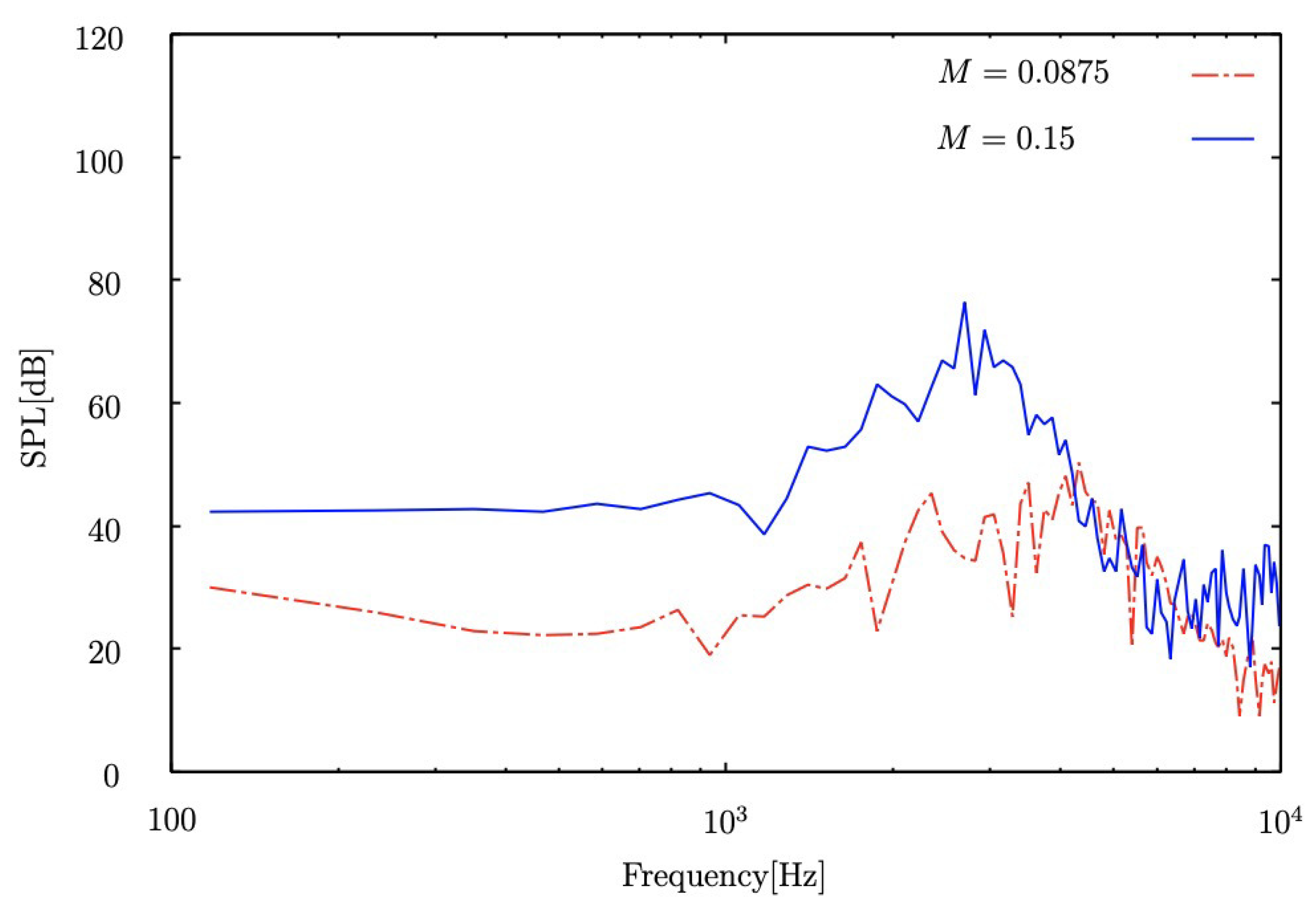
4.2. Comparison of Different Mach Numbers

In this subsection, using the same computational parameters such as Reynolds number $Re=2\times {10}^5$ and the angle of attack $\alpha =9^{\circ }$ in Section 2, we conducted a LES of the turbulent flow field around the NACA0012 airfoil at Mach number $M=0.15$. In order to verify if our acoustic method could reproduce the behavior of sound source due to the variation of Mach number, and, investigate the influence of the increase of Mach number on the acoustic field, the results of the sound field in case of $M=0.15$ are compared with that in case of $M=0.0875$. Figure 8 shows the instantaneous distribution of $\mathsf{\nabla }·\mathit{u}$ around NACA0012 airfoil colored by $|\mathsf{\nabla }·\mathit{u}|\le 0.1$ at Mach numbers $0.0875$ and $0.15$. In the case of $M=0.15$, the remarkable distribution of $\mathsf{\nabla }·\mathit{u}$ was observed near the leading edge in the suction side, while a relatively small distribution was shown in case of $M=0.0875$. From this observation, the compressibility effect due to the increase of Mach number was represented by $\mathsf{\nabla }·\mathit{u}$, and thus the change of the behavior of sound source was reproduced.

Figure 9 shows the instantaneous distribution of $-{\rho }_0\frac{D}{Dt}(\mathsf{\nabla }·\mathbf{u})$ near the leading edge at Mach numbers $M=0.0875$ and $0.15$. The noticeable difference of the distribution for $-{\rho }_0\frac{D}{Dt}(\mathsf{\nabla }·\mathbf{u})$ between Figure 9a,b was not observed in the immediate vicinity of the leading edge. However, in comparison with the case of $M=0.0875$, the clear patterns of $-{\rho }_0\frac{D}{Dt}(\mathsf{\nabla }·\mathbf{u})$ were observed in the circle region in case of $M=0.15$. From this observation, our acoustic theory was proven to be able to reproduce the influence of Mach number on the sound field.

Figure 10 compares the SPL at Mach number $M=0.15$ and $0.0875$ measured at point 1 m from the leading edge in the direction normal to the streamwise direction. Hutcheson et al. [26] measured the aerodynamic noise generated from the flow field around the NACA0015 airfoil under the condition of the angle of attack $\alpha ={10}^{\circ }$, and the Mach number at $M=0.09$, $0.11$, and $0.127$. Their investigation shows that the position of the peak frequency of SPL tends to move from the high-frequency region to the low-frequency region as the Mach number increases. In Figure 10, the maximum peak value obtained by $M=0.15$ is observed in a low frequency region, as it was against the profile of SPL obtained by $M=0.0875$. In other words, the tendency of SPL due to the increase of Mach number is reproduced by our sound source model.

5. Conclusions

Aerodynamic noise from wind turbine blades is one of the major hindrances for the widespread use of large-scale wind turbines to generated green energy. Generally, the weakly compressible turbulent flows around large-scale wind turbine blades that induce the aerodynamic noise, are typical, high Reynolds number flows at low Mach numbers. In order to accurately guide wind turbine blade manufacturers to optimize the blade geometry for aerodynamic noise reduction, an acoustic model that not only understands the relationship between the behavior of sound source and the sound generation but accounts for the compressibility effect, is required. To that end, in this study, a new acoustic theory was proposed, in which we rearranged the continuity and Navier–Stokes equations as a wave equation with a lump of source terms, including the material derivative and square of the velocity divergence. These source terms were used for sound source detection and the estimation of the far-field sound. Our acoustic model was applied to low Mach number, weakly compressible turbulent flows around NACA0012 airfoil. For the computation of flow fields and considering the weak compressibility in flow fields, a LES with the dynamic Smagorinsky subgrid-scale model [28,29] and the CIP-combined unified numerical procedure method [30] was conducted. The reproduced turbulent flow around NACA0012 airfoil was in good agreement with the experimental data. For the estimation of acoustic fields, different acoustic models were performed using our LES database. The distribution of the sources obtained from our acoustic model was compared with the classical sound source models, such as Lighthill [11] and Powell [19] in the case of very low fluctuation of density. The investigation suggested that the derived material derivative of the velocity divergence plays a dominant role as a sound source, and the distribution of our derived source model is consistent with that of the classical sound models. The sound pressure level predicted based on the above-mentioned LES and our newly derived acoustic model was compared with the SPLs calculated from the Lighthill–Curle’s equation [18] employing our LES database and the experimental data by Miyazawa et al. [31]. The results showed that the SPL from our acoustic model was in reasonable agreement with the experimental data. The influence of the increase of Mach number on the acoustic field was investigated. From the observation, our acoustic source model was verified to be capable of treating the influence of Mach numbers on the acoustic field. As a result, noise prediction of the large-scale wind turbine blade using our acoustic source model is more accurate at a low Mach number, and further, can more accurately guide wind turbine blade manufactures to optimize the blade geometry for aerodynamic noise reduction. At this stage, further validation of sound rated by comparisons with experimental data is necessary. But we believe our proposal contributes to the development of computational aeroacoustics for applications in low Mach number turbulent flows, such as large-scale wind turbine blades.

References

1. Bai, W.; Lee, D.; Lee, K. Stochastic dynamic AC optimal power flow based on a multivariate short-term wind power scenario forecasting model. Energies 2017, 10, 2138. [Google Scholar] [CrossRef] [Green Version]
2. Ageborg Morsing, J.; Smith, M.; Ogren, M.; Thorsson, P.; Pedersen, E.; Forssen, J.; Persson Waye, K. Wind turbine noise and sleep: Pilot studies on the influence of noise characteristics. Int. J. Environ. Res. Public Health 2018, 15, 2573. [Google Scholar] [CrossRef] [PubMed] [Green Version]
3. Zhu, W.J.; Shen, W.Z.; Barlas, E.; Bertagnolio, F.; Sorensen, J.N. Wind turbine noise generation and propagation modeling at DTU Wind Energy: A review. Renew. Sustain. Energy Rev. 2018, 88, 133–150. [Google Scholar] [CrossRef]
4. World Health Organization. Burden of Disease from Environmental Noise: Quantification of Healthy Life Years Lost in Europe; World Health Organization, WHO Regional Office for Europe: Copenhagen, Denmark, 2017. [Google Scholar]
5. Onakpoya, I.J.; OSullivan, J.; Thompson, M.J.; Heneghan, C.J. The effect of wind turbine noise on sleep and quality of life: A systematic review and meta-analysis of observational studies. Environ. Int. 2015, 82, 1–9. [Google Scholar] [CrossRef] [PubMed]
6. Wagner, S.; Bareiss, R.; Guidati, G. Wind Turbine Noise; Springer Science & Business Media: New York, NY, USA, 1996. [Google Scholar]
7. Ghasemian, M.; Ashrafi, Z.N.; Sedaghat, A. A review on computational fluid dynamic simulation techniques for Darrieus vertical axis wind turbines. Energy Convers. Manag. 2017, 149, 87–100. [Google Scholar] [CrossRef]
8. Li, Q.A.; Maeda, T.; Kamada, Y.; Murata, J.; Kawabata, T.; Shimizu, K.; Ogasawara, T.; Nakai, A.; Kasuya, T. Wind tunnel and numerical study of a straight-bladed Vertical Axis Wind Turbine in three-dimensional analysis (Part II: For predicting flow field and performance). Energy 2016, 104, 295–307. [Google Scholar] [CrossRef]
9. Chen, Y.; Lian, Y. Numerical investigation of vortex dynamics in an H-rotor vertical axis wind turbine. Eng. Appl. Comput. Fluid Mech. 2015, 9, 21–32. [Google Scholar] [CrossRef] [Green Version]
10. Oerlemans, S. Reduction of wind turbine noise using blade trailing edge devices. In Proceedings of the 22nd AIAA/CEAS Aeroacoustics Conference, Lyon, France, 30 May–1 June 2016. [Google Scholar]
11. Lighthill, M.J. On sound generated aerodynamically I. General theory. Proc. R. Soc. Lond. Ser. A 1952, 211, 564–587. [Google Scholar]
12. Lighthill, M.J. On sound generated aerodynamically II. Turbulence as a source of sound. Proc. R. Soc. Lond. Ser. A 1954, 222, 1–32. [Google Scholar]
13. Sandberg, R.D.; Jones, L.E. Direct numerical simulations of low Reynolds number flow over airfoils with trailing-edge serrations. J. Sound Vib. 2011, 330, 3818–3831. [Google Scholar] [CrossRef]
14. Wolf, W.R.; Lele, S.K. Trailing-edge noise predictions using compressible large-eddy simulation and acoustic analogy. AIAA J. 2012, 50, 2423–2434. [Google Scholar] [CrossRef]
15. Sandberg, R.D.; Sandham, N.D. Direct numerical simulation of turbulent flow past a trailing edge and the associated noise generation. J. Fluid Mech. 2008, 596, 353–385. [Google Scholar] [CrossRef] [Green Version]
16. Bogey, C.; Bailly, C.; Juve, D. Computation of flow noise using source terms in Linearized Euler’s equations. AIAA J. 2002, 40, 235–243. [Google Scholar] [CrossRef] [Green Version]
17. Jawahar, H.K.; Lin, Y.; Savill, M. Large eddy simulation of airfoil self-noise using OpenFOAM. Aircraft Eng. Aerosp. Technol. 2018, 90, 126–133. [Google Scholar]
18. Curle, N. The influence of solid boundaries upon aerodynamic sound. Proc. R. Soc. Lond. Ser. A 1955, 231, 505–514. [Google Scholar]
19. Powell, A. Theory of vortex sound. J. Acoust. Soc. Am. 1964, 36, 177–195. [Google Scholar] [CrossRef]
20. Amiet, R.K. Noise due to turbulent flow past a trailing edge. J. Sound Vib. 1976, 47, 387–393. [Google Scholar] [CrossRef]
21. Wang, M.; Freund, J.B.; Lele, S.K. Computational prediction of flow-generated sound. Annu. Rev. Fluid Mech. 2006, 38, 483–512. [Google Scholar] [CrossRef] [Green Version]
22. Howe, M.S. Theory of Vortex Sound; Cambridge University Press: Cambridge, UK, 2003; Volume 33. [Google Scholar]
23. Möhring, W. On vortex sound at low Mach number. J. Fluid Mech. 1978, 85, 685–691. [Google Scholar] [CrossRef]
24. Takaishi, T.; Ikeda, M.; Kato, C. Method of evaluating dipole sound source in a finite computational domain. J. Acoust. Soc. Am. 2004, 116, 1427–1435. [Google Scholar] [CrossRef]
25. Ewert, R.; Schroder, W. On the simulation of trailing edge noise with a hybrid LES/APE method. J. Sound Vib. 2004, 270, 509–524. [Google Scholar] [CrossRef]
26. Hutcheson, F.V.; Brooks, T.F.; Stead, D.J. Measurement of the noise resulting from the interaction of turbulence with a lifting surface. Int. J. Aeroacoust. 2012, 11, 675–700. [Google Scholar] [CrossRef]
27. Hutcheson, F.V.; Brooks, T.F. Noise radiation from single and multiple rod configurations. Int. J. Aeroacoust. 2012, 11, 291–333. [Google Scholar] [CrossRef] [Green Version]
28. Germano, M.; Piomelli, U.; Moin, P.; Cabot, W.H. A dynamic subgrid-scale eddy viscosity model. Phys. Fluids A 1991, 3, 1760–1765. [Google Scholar] [CrossRef] [Green Version]
29. Lilly, D.K. A proposed modification of the Germano subgrid-scale closure method. Phys. Fluids A 1992, 4, 633–635. [Google Scholar] [CrossRef]
30. Yabe, T.; Wang, P.Y. Unified numerical procedure for compressible and incompressible fluid. J. Phys. Soc. Jpn. 1991, 60, 2105–2108. [Google Scholar] [CrossRef]
31. Miyazawa, M. Large eddy simulation of flow around an isolated aerofoil and noise prediction. In Proceedings of the 5th JSME-KSME Joint Fluids Engineering Conference, Nagoya, Japan, 14–18 July 2002; pp. 546–551. [Google Scholar]
32. Okita, K.; Kajishima, T. Numerical simulation of unsteady cavitating flows around a hydrofoil. Trans. Jpn. Soc. Mech. Eng. Ser. B 2002, 68, 637–644. [Google Scholar] [CrossRef] [Green Version]
33. Kajishima, T.; Ohta, T.; Okazaki, K.; Miyake, Y. High-order finite-difference method for incompressible flows using collocated grid system. JSME Int. J. Ser. B 1998, 41, 830–839. [Google Scholar] [CrossRef] [Green Version]
34. Han, C.; Kajishima, T. Large eddy simulation of weakly compressible turbulent flows around an airfoil. J. Fluid Sci. Technol. 2014, 9, JFST0063. [Google Scholar] [CrossRef]
35. Tang, H.; Lei, Y.; Li, X.; Fu, Y. Large-Eddy Simulation of an Asymmetric Plane Diffuser: Comparison of Different Subgrid Scale Models. Symmetry 2019, 11, 1337. [Google Scholar] [CrossRef] [Green Version]
36. Tang, H.; Lei, Y.; Fu, Y. Noise Reduction Mechanisms of an Airfoil with Trailing Edge Serrations at Low Mach Number. Appl. Sci. 2019, 9, 3784. [Google Scholar] [CrossRef] [Green Version]
37. Tang, H.; Lei, Y.; Li, X.; Fu, Y. Numerical Investigation of the Aerodynamic Characteristics and Attitude Stability of a Bio-Inspired Corrugated Airfoil for MAV or UAV Applications. Energies 2019, 12, 4021. [Google Scholar] [CrossRef] [Green Version]
38. Tamura, A.; Kikuchi, K.; Takahashi, T. Residual cutting method for elliptic boundary value problems. J. Comput. Phys. 1997, 137, 247–264. [Google Scholar] [CrossRef]
Figure 1. The profile of NACA0012 airfoil.
Energies 12 04596 g001
Figure 2. Computational domain and boundary conditions.
Energies 12 04596 g002
Figure 3. Mean pressure coefficient C p .
Energies 12 04596 g003
Figure 4. Mean fluctuation of C p .
Energies 12 04596 g004
Figure 5. Instantaneous, cross-sectional profile of the sound source terms around NACA0012 airfoil at M = 0.0875 : (a) · ( · T ) ; (b) · ( ω × u ) ; (c) ρ 0 D D t ( · u ) ; (d) ρ 0 ( · u ) 2 .
Energies 12 04596 g005
Figure 6. Time evolution of instantaneous and cross-sectional profiles of ρ 0 D D t ( · u ) and ω z near the leading edge at M = 0.0875 : (a,c,e) denote ρ 0 D D t ( · u ) at different moments, where the time interval is 3.5 × 10 2 s; (b,d,f) denote ω z at different moments corresponding to the times of (a,c,e), respectively.
Energies 12 04596 g006
Figure 7. Sound pressure level at M = 0.0875 .
Energies 12 04596 g007
Figure 8. Instantaneous, cross-sectional profiles of · u around NACA0012 airfoil at different Mach numbers: (a) M = 0.0875 ; (b) M = 0.15 .
Energies 12 04596 g008
Figure 9. Instantaneous, cross-sectional profiles of ρ 0 D D t ( · u ) near the leading edge: (a) M = 0.0875 ; (b) M = 0.15 .
Energies 12 04596 g009
Figure 10. Sound pressure level obtained by using ρ 0 · [ ( u · ) u ] at M = 0.0875 and 0.15 .
Energies 12 04596 g010