Abstract
Stochastically fluctuating wind power has an escalating impact on the stability of power grid operations. To smooth out short- and long-term fluctuations, this paper presents a coordinated control algorithm using model predictive control (MPC) to manage a hybrid energy storage system (HESS) consisting of ultra-capacitor (UC) and lithium-ion battery (LB) banks. In the HESS-computing period, the algorithm minimizes HESS operating costs in the subsequent prediction horizon by optimizing the time constant of a flexible first-delay filter (FDF) to obtain the UC power output. In the LB-computing period, the algorithm keeps the optimal time constant of the FDF from the previous period to directly obtain the power output of the UC bank to minimize the power output of the LB bank in the next prediction horizon. A relaxation technique is deployed when the problem is unsolvable. Thus, the fluctuation mitigation requirements are fulfilled with a large probability even in extreme conditions. A state-of-charge (SOC) feedback control strategy is proposed to regulate the SOC of the HESS within its proper range. Case studies and quantitative comparisons demonstrate that the proposed MPC-based algorithm uses a lower power rating and storage capacity than other conventional algorithms to satisfy one-minute and 30-min fluctuation mitigation requirements (FMR).
1. Introduction
Wind energy is an inexhaustible and environmentally friendly source of renewable energy. Countries like China, USA, Germany, and Spain have led in the installation capacities of wind energy in global markets. During the last decade, China shared the highest wind energy capacities in the world. The Chinese government has been providing attractive policies for local wind energy manufacturing companies and developers [1]. A comprehensive assessment of the production of energy from wind has identified a grid-integrated wind generation potential of 11.9–14% of China’s projected energy demand by 2030 [2].
However, fluctuations in energy due to the intrinsic stochastic nature of wind can pose significant challenges for power grids, especially when a significant amount of wind power must be integrated into existing power networks [3]. To maintain stable operations, electric power utilities have published technical requirements for the connections of wind farms into power grids [4,5,6].
Energy storage is one of the most promising and practical techniques for mitigating wind power fluctuations [7,8], with different storage technologies with characteristics that are vastly differing. Many systems deploy batteries in a complementary mode with other storage devices, such as ultracapacitors for compensation of fluctuating output in different timeframes. A common system of this type is a battery-ultracapacitor-based hybrid energy storage system (HESS) [9,10]. Generally, ultracapacitors have higher power capacity than battery energy storage, while batteries provide higher energy density [9]. Since energy storage size determines the cost of the HESS, it becomes imperative that the control method of the HESS should be tailored to minimize the required energy storage. In this paper, we introduce a coordinated control algorithm for a HESS composed of a high power density ultra-capacitor (UC) bank and a high energy density lithium-ion battery (LB) bank.
A first-delay-filter (FDF) is conventionally applied to perform the online charge/discharge control of energy storage [11,12], since it is suitable for real-time application due to its rapid computational speed. However, FDF filters lead to overcompensation due to their inertia feature, which can further deteriorate a system’s capability to cope with wind power variations. Tanabe et al. [4] and Xiangjun et al. [13] combined an FDF with a rate limiter to ensure that wind farm power fluctuations still met the required technical requirements, while a flexible FDF with time constant optimization to limit the power fluctuation under restriction has also been proposed. Some studies have adopted algorithmic approaches to energy storage systems (ESS) or HESS scheduling. Abbey et al. utilized a knowledge-based control approach [14], while Datta et al. implemented fuzzy logic to smooth power fluctuations of photovoltaic-diesel hybrid power system [15]. However, these methods are all based on an FDF, and fail to guarantee that the smoothing power output at the point of interconnection of wind farm always fulfills the fluctuation mitigation requirements (FMR).
In a previous work, we presented a wavelet-based scheme to control a HESS [5], which provides a lower required storage capacity than the required capacity calculated for FDF-based techniques. Using a model predictive control (MPC) is another effective solution owing to its superior handling capability of constraints in order to mitigate wind power fluctuations. MPC has gained popularity in industry since the 1990s and has become a major success story in modern control engineering [16]. In this paper, the main contribution is the proposal of a MPC-based rolling optimization control strategy for a HESS in the presence of practical constraints, consisting of two types of computing periods (HESS-computing and LB-computing periods). At each time step, a quadratically-constrained programming (QCP) problem is solved to minimize the cost of HESS or LB in the next prediction horizon. It effectively mitigates wind power fluctuations in multiple time scales, and with a novel state-of-charge feedback (SOCFB) control scheme, it can also effectively restore the SOCs of the HESS to its proper safety range.
2. Fluctuation Mitigation Requirements for Wind Power Integration
2.1. Composition of Wind Power Signals
Figure 1 illustrates a conceptual drawing of the Wind/HESS hybrid power generation system architecture. The system consists of a wind farm, an MPC-based coordinated controller, and a HESS comprised of a UC bank and a LB bank. At time k, the controller monitors the wind power , allocates the charge/discharge reference values and in real-time, and passes these values to the corresponding DC/AC power converter controllers. Therefore, the combined power output would be the combination of actual output , , and the wind park power output .
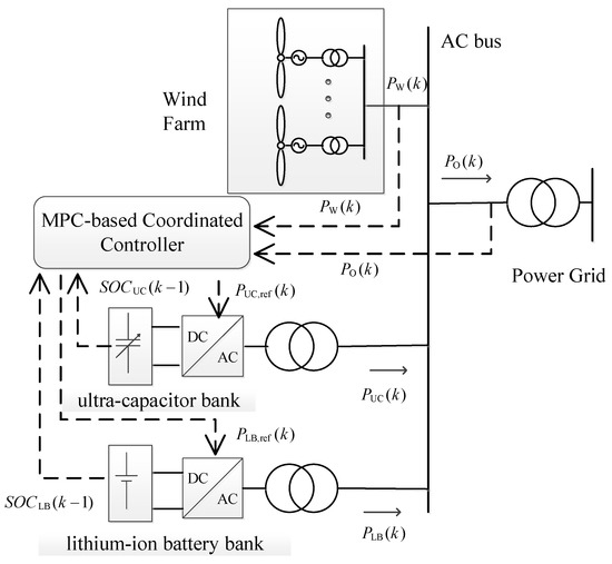
Figure 1.
Diagram of a wind/HESS hybrid power generation system.
2.2. Fluctuation Mitigation Requirements
Power fluctuations at different time scales impact differing aspects of power system operation. Fluctuations within time frames of a few minutes to several hours affect system generation reserves [17], while fluctuations on the seconds to minutes time scale influence ancillary services, such as frequency regulation, spinning reserves, voltage support, black-start capacity, and so on [18]. These fluctuations should be limited with the increased level of wind penetration in order to still integrate as large an amount of wind power generation as possible into the electricity grid while reducing any impact on power system stability [19]. The German (E.ON) requires a maximum ramping rate of 10% of connection capacity per minute specification for wind power systems, and in Ireland there are two specified settings—ramping rate per minute and ramping rate over 10 min [3]. In Japan, two requirements are published by Tohoku Electric Power Company—2% of the rated power per minute and 10% of the rated power per 20 min [4]. In recent years, several fluctuation mitigation requirements (FMR) have been studied by electric power utilities in China [5,6]. For this work, we have selected two of the FMRs in force in China as follows:
2.2.1. One-Minute Fluctuation Mitigation Requirements
The maximum fluctuation range of in any one-minute evaluation window should be limited to within of .
2.2.2. Thirty-Minute Fluctuation Mitigation Requirements
The maximum fluctuation range of in any 30-min evaluation window should be limited to within of .
3. MPC-Based Coordination Control Model
3.1. Flow Chart of MPC-Based Coordination and Optimization Control
A detailed flowchart of the complete MPCCC process for the HESS is provided in Figure 2. MPC is a form of control where the current control action is obtained by solving, online, a finite horizon open-up optimal control problem at each sampling instant where a receding horizon approach is implemented [20]. Using the current state x(k) at time k as the initial state, an open loop optimal control problem is solved over some future interval by taking into account the current and future constraints. The MPC algorithm yields an optimal control sequence, and the first value in this sequence is injected into the plant. This procedure is then repeated at time (k+1) using the current state x(k+1).
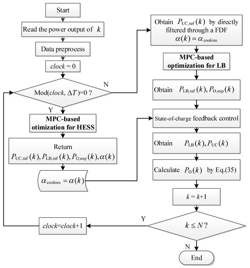
Figure 2.
Flowchart of the complete MPC-based coordination control process for the HESS.
The goal of a HESS control system is to satisfy any FMRs using the smallest energy storage system possible. Our proposed MPC-based coordination control (MPCCC) is a novel method for controlling a HESS, whose basic principle is illustrated in Figure 3. This control system deploys a flexible FDF to obtain the charging/discharging reference value of the UC bank . The corresponding time constant of FDF , the charging/discharging reference value for LB , and the expected combined output are obtained by solving the optimization problem of the MPCCC.
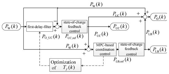
Figure 3.
Block diagram of the proposed MPC-based coordination control algorithm.
However, it is time-consuming and cumbersome to optimize in each sampling period. Instead, is only optimized for every period based on ultra-short-term wind power forecasts by solving the MPCCC model for the HESS. This is referred to as the HESS-computing period. In LB-computing periods, the optimal time constant is instead kept from the last computing period to directly get . The goal of this stage is to minimize in the next control horizon, which degenerates to the MPCCC model for controlling the LB bank. We propose using a state-of-charge feedback (SOCFB) control strategy to regulate the SOC of both banks of the HESS within their proper ranges.
The concrete modelling process is described in the following subsections.
3.2. Flexible First-Delay-Filter with Variable Time Constant
As shown in Figure 2, the transfer function model of the first-delay-filter (FDF) is:
where is the combined output of and . The reference value of the UC bank is regulated to:
A recurrence formula for and are obtained via the discretization of Equations (1) and (2), given by:
where is the time step. we set s for this paper.
The theoretical range of is , which is difficult to optimize. Defining a constant , Equation (3) can be rewritten as:
where, obviously, . When , the UC bank is out of use, indicating that all fluctuations should be mitigated by the LB bank, which is economically feasible. Since a UC’s “best fit” frequency band is , where and [21], we can set , where . Substituting Equation (5) into Equation (4), we obtain:
Here, is an increasing function of , which means optimizing is equivalent to optimizing , where a larger leads to more power being absorbed by the UC bank and thus providing a smoother output.
3.3. Capacity Calculation
The energy state of the UC and LB storage systems at time k, representing the energy content in it, are given by:
where and are the initial energy states.
The SOC of the battery can be measured by integrating the battery current over time:
where is the corresponding conversion efficiency and is the rated energy capacity of the battery. Thus, Equation (9) can provide both and for the system.
The energy storage capacity used for damping fluctuations of the UC and LB banks, i.e., and , respectively, are then defined as:
where N is the total number of time points in the data sample.
3.4. MPC-Based Coordination Control Model
3.4.1. MPC-Based Coordination Control Model for the HESS
For the HESS-computing period, we formulate the optimization model to obtain the optimal combined power output of the HESS and the wind system that meets all FMRs. The cost of HESS usage in the subsequent control horizon is tightly related to the operational economy and should be minimized.
(1) Objective function
With this relationship in mind, we can express the objective function of the optimization model as:
where , , , and are penalty coefficients associated with the power and energy costs of the storage system, M is the control horizon, and and are optimizing control variables. Thus, the goal consists of reducing the power and energy penalties associated with using the HESS.
(2) Equality constraints: power balance constraint
where , and FDF constraint:
where . Note that there exists a coupling of the optimization variables and in Equation (14), making the formula a quadratically constrained quadratic programming (QCQP) problem.
Power balance constraint of the UC bank:
where .
(3) Inequality constraints: FMR constraints
where . The combined output should simultaneously meet the FMRs of both time scales.
Output power constraints:
where .
HESS power constraints:
Here, , and , , , and are the maximum charging and discharging power of the UC and LB banks, respectively, such that:
where and is the charge and discharge time. , , , and are determined when designing the capacity configuration of the HESS.
HESS energy constraints:
3.4.2. MPC-based control model for the LB bank
During the LB-computing period, the optimization model is established to obtain the optimal output of LB and combined power output meeting all FMRs. The goal is to minimize the cost of LB utilization in the subsequent control horizon.
(1) Objective function
where . Note that is the optimizing variable.
(2) Equality and inequality constraints
The equality and inequality constraints can be derived from Equations (13)–(27) when is constant in this period.
3.5. Transformation of the FMR Constraints
Since the FMR constraints in Equations (16) and (17) contain max-min operators, they make it difficult to solve the MPCCC problem. To ease computational requirements, the FMR constraints should be equivalently converted into linear constraints, and the FMR interval [5] expanded as the upper and lower limits of , i.e.,:
for 1-min FMR, where and . This preprocessing improves the solution efficiency.
3.6. Model Solution
Suppose is a variable vector containing all states and controls, where:
for the HESS-computing period, and:
for the LB-computing period, respectively. Note that PUC, PLB, PO, and PO_UC are all M-dimensional vectors, and PLB, PO and are controllable.
We can then formulate the MPCCC problem in a general nonlinear programming form:
where is the diagonal weighting matrix and describes the linear part of the objective function, whereas the matrix H and the vector h describe the equality constraints. and are the lower and upper bound of the inequality constraints.
Note that the quadratically-constrained programming (QCP) problem of Equation (32) is readily solved using the interior point methods. In this work, we solve the optimization problem at each time step using IPOPT (Interior Point OPTimize) in MATLAB. IPOPT is a software package for large-scale nonlinear optimization [22], which is available from the COIN-OR initiative and written in C++ and is released as open source code under the Eclipse Public License (EPL).
3.7. Feasibility and Constraints Handling
MPCCC problems can become unsolvable when a large disturbance occurs (i.e., extreme weather conditions, batteries are depleted, and other conditions that violate the constraints in Equations (16) and (17)). In this case, the constraints should be relaxed by introducing slack variables such that the constraints are always feasible. Meanwhile, the objective function is modified by introducing a term that penalizes the magnitude of the constraint violations. Hence, the MPCCC problem in Equation (32) is modified to:
where and are slack vectors for the equality and inequality equations, respectively, and and are the corresponding penalty factors that are nonzero only if the equation is violated.
Clearly, the relaxed MPCCC problem is still a QCP problem, and so can be solved efficiently. Thus, feasibility is ensured by increasing the size of the optimization problem.
3.8. State-of-Charge Feedback Control
HESS control strategies should take into consideration the SOC status and maximum available charge or discharge power constraints of the storage system. Here, the SOC feedback control strategy is presented to regulate the SOC of the batteries within proper range of 20%–80% (charge/discharge safety interval).
3.8.1. State-of-Charge Feedback Control of the UC
The UC bank’s power reference value should be limited within the UC power constraint dictated in Equation (20).
3.8.2. State-of-Charge Feedback Control of the LB
is obtained through the SOCFB. The power reference of the LB is calculated by:
To determine, we employ an interval narrowing method considering long-term operations. The procedure is briefly as follows:
Working Stage 1: Let and . Figure 4 outlines the SOCFB, expressed stepwise below:
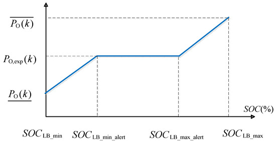
Figure 4.
Basic principle of SOC feedback control for the LB.
(1) If , then set to a smaller value.
(2) If , then set to a larger value.
(3) If , the LB strictly responds with the reference value from Equation (34).
As a result, the target combined output can be adaptively modified according to the charging-level of the LB.
Working Stage 2: Compute when the LB bank reacts to the reference value obtained from Stage 1. Then let = 20% and = 80%. Repeat Stage 1, updating with the value of .
Working Stage 3: Then the combined output is determined as:
4. Simulation and Analysis
4.1. HESS Capacity and Power Configurations
The aim of this section is to estimate the power rating demand and capacity for the HESS that can achieve all FMRs using the proposed method. Thus, SOCFB is not considered at this stage.
Figure 5 demonstrates three typical days (separated into three different cases) of wind power output with 1-s time resolution from the wind energy database of a wind farm in China. The rated capacity of the wind farm is 6 MW.
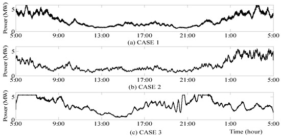
Figure 5.
The wind power output sampled with 1-s resolution.
Denote the average fluctuation as , the maximum fluctuation as F1max, and the standard deviation of power fluctuations in every one-minute interval as ρ1. Similarly, , F30max, and ρ30 can be defined for power fluctuations over a 30-min interval. The statistical analysis results for each of the three representative cases are given in Table 1.

Table 1.
Statistical analysis of cases.
To show the effectiveness of the proposed MPCCC algorithm, we derived the minimal HESS power rating and capacity required during a single day for the MPCCC algorithm, then did the same for a basic FDF [23], an FDF with a rate limiter [4,13], and a wavelet-based sizing algorithm [5]. The solutions are further displayed in Table 2.
Table 2.
Capacity configuration solution with different sizing methods.
4.2. Comparison of MPCCC and Conventional Algorithms
We simulated the real-time control of a wind power system using a HESS to evaluate the performance of our proposed algorithm, using four different indices to better evaluate the different control strategies and to investigate the benefits of the MPCCC algorithm. The indices are:
4.2.1. Maximum Absolute Value of the Energy Storage Power Output
Note that the cost of the power conversion system equipment is in proportion with the power rating of the system.
4.2.2. Energy Storage Capacity Consumed
The cost of the storage unit is in proportion with the amount of energy it must use.
4.2.3. Battery Health Index
The battery health index (BHI) assesses the effectiveness of utilizing the storage systems within the specified safety range, as defined by:
where N is the total number of time points in the data sample; is a 0–1 variable defined as:
A larger BHI indicates a more effective SOCFB.
4.2.4. Equivalent Full Cycle
At the end of a simulation using one of the specified control strategies, the total fractional damage D was calculated to predict the expected life of the HESS [24]:
where is cycle to failure—which is a function of depth of discharge (DOD) and the corresponding number of cycles provided in the datasheets [11]—and is the corresponding number of cycles fulfilled at that DOD. Note that the reciprocal of D is the expected life of the battery.
For our study, we must rewrite Equation (38) as:
Here, , where and are the SOC at battery stop and start for the k-th discharging process.
Note that the discharge/charge cycling of the batteries is irregular when using the batteries to smooth wind power output. Therefore, we propose using an equivalent full cycle EFC in this paper to determine D for the different methods:
Substituting Equation (40) into Equation (39), we can solve for EFC:
We compared the results from our MPCCC algorithm with the results from a basic FDF [9], a FDF with a rate limiter [4,13], and a wavelet-based control algorithm (OWCC) developed in [3]. The rate limit was set to ±7%/1800. The related penalty coefficients were derived from [25], where and . Table 3 and Table 4 give the results from the three cases.
Table 3.
Comparison of different control methods (I).
Table 4.
Comparison of different control methods (II).
Clearly, the basic FDF applies the most energy storage of all the algorithms given the same sizing solution, while by adopting the proposed OWCC scheme, the required storage capacity and power rating can be kept at lower levels. In Case 1, the is 24.55% of the capacity used with the basic FDF, 44.60% of the FDF with a rate limiter, and 74.58% of that of the OWCC. In addition, the is 85.04% smaller for the MPCCC scheme compared to results employing the basic FDF. In terms of life expectancy, the expected life of the LB using MPCCC is 2.5 times longer than a system using FDF, 1.93 times that of a system using a rate limiter, and 1.14 times that of a system implementing OWCC. It is noted that the MPCCC algorithm adopts a flexible FDF to compute the power reference value, which can take advantage of the high power density of the UC bank, which allows for the MPCCC-based system to have the largest of the tested algorithms. Furthermore, the MPCCC scheme essentially allocates the charging/discharging reference value of the HESS through frequency distribution by employing the flexible FDF. This separation of use improves the lifetime of both types of storage devices [9].
To further investigate the necessity of the SOCFB, we compared two different MPCCC schemes: namely, MPCCC-BA, corresponding to the basic MPCCC without the SOCFB and MPCCC, which is the proposed complete MPCCC scheme. For this experiment, we used the MPCCC-based one-day capacity configuration solution in Table 2.
As shown in Table 5, using the SOCFB consumes 7% more LB bank capacity compared to the MPCCC-BA system, since the SOCFB in the MPCCC additionally charges/discharges the HESS according to the SOCs of each of the banks. However, the BHI of the LB bank increases by 84%, which will prolong the lifetime of the HESS and ensures enough energy storage for long-term mitigation.
Table 5.
Comparison of different MPCCC methods.
4.3. Verification of the Proposed Control Strategy
In this section, the power profile of Case 1 was applied to verify the effectiveness of the proposed control strategy. For this experiment, the computation cycle of the HESS-computing period was 10 s. To validate the effectiveness of the proposed SOCFB, the initial SOC states of the UC and LB banks were set to 65% and 75%, respectively. As this paper focuses mainly on MPC-based coordinated control of a HESS, neither inverter control specifics nor the related issues were considered. Simulation results were obtained using MATLAB and accordingly displayed in Figure 6, Figure 7, Figure 8 and Figure 9.
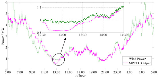
Figure 6.
Wind power output and the smooth output of the MPC-based control algorithm.
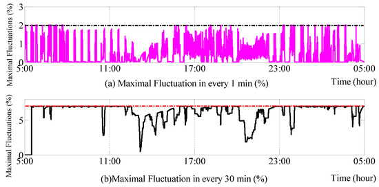
Figure 7.
Maximal fluctuations of the smoothed output in two time-scales.
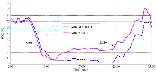
Figure 8.
State-of-charge curves of the lithium-ion battery bank.
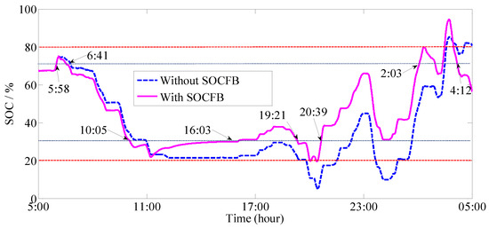
Figure 9.
State-of-charge curves of the ultra-capacitor bank.
It can be seen in Figure 6 that the power fluctuations were effectively smoothed by means of the proposed MPCCC algorithm. Figure 7 reveals the maximum smoothed power output fluctuations in both time scales. As the figure makes clear, the fluctuations were effectively restricted below the limit value of 2% per min and 7% per 30 min.
Figure 8 and Figure 9 show that the SOCFB of the LB and UC banks effectively kept the SOCs between 20% and 80% for most periods during the entire observed sample. For example, when the SOC of the LB bank went above 70% at about 5:00 am or under 30% at about 9:50 am, the SOCFB would adaptively work to adjust the power reference value. In contrast, another time-domain simulation without SOCFB was also performed, and the SOC curves frequently deviated from the expected safety range. Hence, the proposed SOC feedback control can achieve good management of the SOCs of the LB and UC banks, which would enhance the reliability of long-term operation.
Furthermore, the average computing CPU time in each step size is 0.0263 s. Since the time step in this paper is 1 s, the calculation speed is sufficient to satisfy real-time operation requirements.
5. Conclusions
The main contributions of this paper are:
- A novel MPC-based coordinated control strategy consisting of HESS-computing and LB-computing periods is developed. At each time step, we solve a QCP problem using IPOPT in MATLAB. In the HESS-computing periods, the goal is to minimize the cost of HESS in the next prediction horizon, the optimal power output of LB is obtained, as well as the optimal time constant of first-delay filter for obtaining the power output of UC. In the LB-computing period, the optimal time constant in the last HESS-computing period is kept to directly obtain the power output of UC, the goal of this stage is simplified to minimize the cost of LB utilization in the subsequent control horizon. This control strategy effectively mitigates wind power fluctuations in multiple time scales;
- Adopted a flexible FDF with an optimization of the time constant to obtain the reference value of the UC bank, which can take the full advantage of the high power density of the UC bank;
- Allocated the charge/discharge instruction value of the HESS based on frequency distribution by employing the flexible FDF. This improves the lifetime of both storage devices;
- Deployed a relaxation technique when the MPCCC problem is unsolvable. Thus, the FMR is fulfilled with a large probability even in extreme conditions; and
- Presented a novel SOCFB control scheme that effectively restores the SOCs of the HESS to its proper safety range.
This scheme resulted in required storage ratings that are lower than the ratings calculated using previous published techniques.
Author Contributions
Conceptualization, Methodology, Supervision and Funding, Q.J.; Validation, Formal Analysis, Investigation, Resources, Data Curation, Writing—Original Draft Preparation and Writing—Review & Editing, H.H.
Funding
This work was supported by National High Technology Research and Development Program of China (Grant No. 2011AA05A113) and National Basic Research Program of China (Grant No. 2012CB215106).
Conflicts of Interest
The authors declare no conflict of interest. The funders had no role in the design of the study; in the collection, analyses, or interpretation of data; in the writing of the manuscript, and in the decision to publish the results.
References
- Sahu, B.K. Wind energy developments and policies in China: A short review. Renew. Sustain. Energy Rev. 2018, 81, 1393–1405. [Google Scholar] [CrossRef]
- Yuan, J. Wind energy in China: Estimating the potential. Nat. Energy 2016, 1, 16095. [Google Scholar] [CrossRef]
- Fox, B.; Flynn, D.; Bryans, L.; Jenkins, N.; Milborrow, D.; O’Malley, M.; Watson, R.; Anaya-Lara, O. Wind power integration: Connection and system operation aspects. IET Power Energy Ser. 2006, 50, 2007. [Google Scholar]
- Tanabe, T.; Sato, T.; Tanikawa, R.; Aoki, I.; Funabashi, T.; Yokoyama, R. Generation scheduling for wind power generation by storage battery system and meteorological forecast. In Proceedings of the 2008 IEEE Power and Energy Society General Meeting—Conversion and Delivery of Electrical Energy in the 21st Century, Pittsburgh, PA, USA, 20–24 July 2008; pp. 1–7. [Google Scholar]
- Jiang, Q.; Hong, H. Wavelet-Based Capacity Configuration and Coordinated Control of Hybrid Energy Storage System for Smoothing Out Wind Power Fluctuations. IEEE Trans. Power Syst. 2013, 28, 1363–1372. [Google Scholar] [CrossRef]
- Jiang, Q.; Wang, H. Two-Time-Scale Coordination Control for a Battery Energy Storage System to Mitigate Wind Power Fluctuations. IEEE Trans. Energy Convers. 2013, 28, 52–61. [Google Scholar] [CrossRef]
- Díaz-González, F.; Sumper, A.; Gomis-Bellmunt, O.; Villafáfila-Robles, R. review of energy storage technologies for wind power applications. Renew. Sustain. Energy Rev. 2012, 16, 2154–2171. [Google Scholar] [CrossRef]
- Eyer, J.; Corey, G. Energy Storage for the Electricity Grid: Benefits and Market Potential Assessment Guide; Sandia National Laboratories: Albuquerque, NM, USA, 2010. [Google Scholar]
- Onar, O.C.; Uzunoglu, M.; Alam, M.S. Dynamic modeling, design and simulation of a wind/fuel cell/ultra-capacitor-based hybrid power generation system. J. Power Sources 2006, 161, 707–722. [Google Scholar] [CrossRef]
- Thounthong, P.; Raël, S.; Davat, B. Control Strategy of Fuel Cell and Supercapacitors Association for a Distributed Generation System. IEEE Trans. Ind. Electron. 2007, 54, 3225–3233. [Google Scholar] [CrossRef]
- Henson, W. Optimal battery/ultracapacitor storage combination. J. Power Sources 2008, 179, 417–423. [Google Scholar] [CrossRef]
- Paatero, J.V.; Lund, P.D. Effect of energy storage on variations in wind power. Wind Energy 2005, 8, 421–441. [Google Scholar] [CrossRef]
- Hadjipaschalis, I.; Poullikkas, A.; Efthimiou, V. Overview of current and future energy storage technologies for electric power applications. Renew. Sustain. Energy Rev. 2009, 13, 1513–1522. [Google Scholar] [CrossRef]
- Abbey, C.; Strunz, K.; Joos, G. A knowledge-based approach for control of two-level energy storage for wind energy systems. IEEE Trans. Energy Convers. 2009, 24, 539–547. [Google Scholar] [CrossRef]
- Datta, M.; Senjyu, T.; Yona, A.; Funabashi, T. A fuzzy based method for leveling output power fluctuations of photovoltaic-diesel hybrid power system. Renew. Energy 2011, 36, 1693–1703. [Google Scholar] [CrossRef]
- Richalet, J. Industrial applications of model based predictive control. Automatica 1993, 29, 1251–1274. [Google Scholar] [CrossRef]
- Sorensen, P.; Cutululis, N.A.; Vigueras-Rodriguez, A.; Jensen, L.E.; Hjerrild, J.; Donovan, M.H.; Madsen, H. Power fluctuations from large wind farms. IEEE Trans. Power Syst. 2007, 22, 958–965. [Google Scholar] [CrossRef]
- International Electrotechnical Commission. Grid Integration of Large-Capacity Renewable Energy Sources and Use of Large-Capacity Electrical Energy Storage, Market Strategy Board. October 2012. Available online: http://www.iec.ch/whitepaper/pdf/iecWP-gridintegrationlargecapacity-LR-en.pdf (accessed on 1 September 2019).
- Bonneville Power Administration. Renewable Energy Technology Roadmap, Technology Innovation Office. September 2006. Available online: http://www.bpa.gov/corporate/business/innovation/docs/2006/RM-06_Re-newablesFinal.pdf (accessed on 5 September 2019).
- Mayne, D.Q.; Rawlings, J.B.; Rao, C.V.; Scokaert, P.O. Constrained model predictive control: Stability and optimality. Automatica 2000, 36, 789–814. [Google Scholar] [CrossRef]
- Schoenung, S. Characteristics and Technologies for Long-vs. Short-term Energy Storage; Sandia Report SAND2001-0765; United States Department of Energy: Washington, DC, USA, 2001. [Google Scholar]
- Mehrotra, S. On the implementation of a primal-dual interior point method. SIAM J. Optim. 1992, 2, 575–601. [Google Scholar] [CrossRef]
- Ise, T.; Kita, M.; Taguchi, A. A hybrid energy storage with a SMES and secondary battery. IEEE Trans. Ind. Appl. 2005, 15, 1915–1918. [Google Scholar] [CrossRef]
- Manwell, J.F.; Rogers, A.; Hayman, G.; Avelar, C.T.; McGowan, J.G.; Abdulwahid, U.; Wu, K. Hybrid2: A Hybrid System Simulation Model: Theory Manual; National Renewable Energy Laboratory: Amherst, MA, USA, 1998. [Google Scholar]
- Jiang, Q.; Gong, Y.; Wang, H. A Battery Energy Storage System Dual-Layer Control Strategy for Mitigating Wind Farm Fluctuations. IEEE Trans. Power Syst. 2013, 28, 263–3273. [Google Scholar] [CrossRef]


© 2019 by the authors. Licensee MDPI, Basel, Switzerland. This article is an open access article distributed under the terms and conditions of the Creative Commons Attribution (CC BY) license (http://creativecommons.org/licenses/by/4.0/).