An Improved Constrained Order Optimization Algorithm for Uncertain SCUC Problem Solving

Abstract

Studying the faster and more efficient method of solving the uncertain security-constrained unit commitment (SCUC) problem is an urgent need for the development of power systems under the background of large-scale wind power access and power dispatching. This study proposes an improved constrained order optimization (COO) algorithm to solve the uncertain SCUC problem. First, the data-driven discrete variable identification strategy is incorporated into the COO rough model, and then, the invalid security constraints identification strategy is incorporated into the COO accurate model. Finally, the improved COO algorithm combines the discrete variable identification with the invalid security constraint identification to make the uncertain SCUC decision. The results of the IEEE 118-bus test system showed that, compared with the traditional COO algorithm, the improved COO algorithm proposed has higher accuracy and better efficiency.

1. Introduction

The security-constrained unit commitment (SCUC) considering uncertain factors has become the most significant and hottest research topic in the power market, given large-scale wind power access [1,2,3]. The uncertain SCUC model has always been considered as a high-dimensional, strongly random, nonlinear NP-hard problem due to the integration of uncertain factors, discrete variables, and safety constraints, including power flow calculations [4,5,6]. Therefore, it is difficult to solve the problem accurately and efficiently. Currently, the problem of solving accurately and efficiently has become a key technical bottleneck in the field of SCUC decision-making [7]. Thus, it is of great theoretical and practical significance to research a more efficient method for solving the uncertain SCUC models.

In recent years, the idea of combining the benders decomposition method with a mature mixed integer programming algorithm has gradually become the mainstream solution of the SCUC problem [8,9,10]. The method first decouples the SCUC model and then solves the decoupled subproblems by utilizing a mixed integer programming algorithm. Benders decomposition method achieves good results in solving the deterministic SCUC model. The difficulty of solving the SCUC model is reduced by decoupling the complex constraints into independent optimization subproblems in the benders decomposition method. However, the effect is not obvious for the problem of scene explosion in SCUC solution caused by the uncertainties. Therefore, its advantages are not obvious when this method is used to solve the uncertain SCUC problem. The constrained order optimization (COO) algorithm [11] was introduced first for the problem of SCUC solving in [12], and a solution of the uncertain SCUC was proposed based on the COO algorithm. From the perspective of the solution space, the feasible region scale of the SCUC model is reduced by constructing the COO rough model. On the basis of the COO rough model, a COO accurate model is constructed to find a good enough solution for the SCUC problem. Compared with the traditional benders decomposition method, the efficiency of the COO algorithm is enhanced to nearly 10 times [12]. Based on the existing researches, the COO algorithm has been proven to be an effective method to solve uncertain SCUC problems rapidly. Although the traditional COO algorithm reduces the scale of the feasible region from the perspective of solution space, elimination and discrimination of the redundant information in the model itself are neglected. Therefore, the traditional COO algorithm can still be improved in terms of the solving efficiency, as described below.

1) When the SCUC model is solved by the traditional COO algorithm, the COO rough model should be constructed first, and then it is used to screen out the feasible solution space for the start–stop state of all units. However, there are many units in large-scale power systems, so the solving efficiency of the COO rough model is not high. The maximum load usually reaches 70% or higher of the installed capacity in the real large power grids, which means some units are always on or off during the scheduling period. Actually, there is no need to consider these constant units during the solving process. Consequently, if the constant units are identified first in the COO rough model, the efficiency of the COO algorithm will be improved. The problem of discrete variable identification has been studied. A linear screening model was constructed to identify the constant units in [13]. The constant units were identified through the priority method in [14,15]. In reference [16], the constant units are identified according to the relationship between the calculated active power output value and the identification rate parameter value. On the whole, the existing methods of the SCUC discrete variable identification are mainly based on the physical model driver idea, that is, constructing a complex mathematical model based on physical principles. However, it is difficult to construct an accurate mathematical model, and the identification results in the existing methods often have the problems of strong subjectivity and low accuracy. In fact, a large amount of structured historical data can be accumulated once the SCUC decision-making scheme is utilized in real power systems. In the long run, the accumulated historical SCUC decision-making scheme also has a guiding significance for the identification of the constant units. Therefore, the idea based on a data-driven method is a feasible way to address the problems of low accuracy and low objectivity of the discrete variable identification strategy.

2) Checking and computing network security constraints are one of the most computationally intensive tasks in solving SCUC problems. The strategy of checking all lines one by one was adopted in the COO accurate model in reference [11]. This strategy will have a serious impact on the computational efficiency of the COO algorithm as the number of nodes and checked lines increases sharply with the expansion of the power grid scale. Reference [17] showed that only a few of the network security constraints are effective that play a role in limiting the feasible region. Furthermore, a fast identification strategy for the invalid security constraints was also proposed. The method in [17] reduces the invalid security constraints by more than 85% without affecting the calculation accuracy of the model. Thus, the identification strategy for the invalid security constraints can reduce the redundancy of the SCUC model. If this method can be introduced in the COO accurate model, the computational efficiency of the COO algorithm will be improved greatly.

In summary, a data-driven discrete variable identification strategy for the SCUC model is proposed in this paper. This strategy and the invalid security constraint identification strategy are used to improve the traditional COO algorithm [12]. Finally, an improved COO algorithm for uncertain SCUC problem solving is proposed. This study is following three steps: construct a COO rough model with the discrete variable identification, construct an accurate COO model with the invalid safety constraint identification, solve the two models separately. The results based on IEEE 118-bus show that the redundancy of the uncertain SCUC model can be reduced effectively, and the computational efficiency can be further improved for the proposed improved strategy.

The main contributions in this study are as follows.

(1) A data-driven strategy of the SCUC discrete variable identification is proposed, and a COO rough model is constructed based on this strategy.

(2) A COO accurate model is constructed based on an identification strategy of the invalid security constraints.

(3) An improved COO algorithm suitable for the problem of SCUC solving is proposed based on the discrete variable identification strategy and the invalid security constraints identification strategy.

The rest of this paper is organized as follows. The SCUC model considering the uncertainty of wind power output is constructed in Section 2. An overall framework for an improved COO algorithm is proposed in Section 3. An improved strategy for the COO algorithm is proposed in Section 4. The simulation analysis is shown in Section 5. Finally, the conclusions are provided in Section 6.

2. The SCUC Model Considering the Uncertainty of Wind Power Output

2.1. Description of the Uncertainty of Wind Power Output

The confidence interval of active power for wind power output is adopted to characterize the uncertainty of wind power output in this study. The interval can be calculated according to the prediction values and error distribution for the wind power output. The specific mathematical expressions are as follows:

$$P_W=\left\{P_{Wjt}{}^{-}\le P_{Wjt}\le P_{Wjt}{}^{+}\right\},$$

(1)

$$P_{Wjt}{}^{-}=P_{Wjt}{}^{*}-K·{\sigma }_{jt},$$

(2)

$$P_{Wjt}{}^{+}=P_{Wjt}{}^{*}+K·{\sigma }_{jt}.$$

(3)

The relationship between K and ζ is as follows, according to the central limit theorem [18].

$$K={\mathsf{\Phi }}^{-1}\left(\frac{1+\zeta }{2}\right)$$

(4)

where P_W represents the active power output from wind power unit. P_Wjt represents the real value of active power output from unit j at time t. P_Wjt^* represents the expected value of active power output from unit j at time t. P_Wjt^- and P_Wjt⁺ represent the lower limit and upper limit respectively of active power output from unit j at time t. ζ represents the confidence probability of wind power output interval. K represents the coefficient relating to confidence probability ζ. σ_jt represents the standard deviation of predicted error of active power output from unit j at time t. Φ^-1 represents the inverse function of the probability density function of the wind power output.

2.2. SCUC Model Based on the Robust Optimization

The uncertainty of wind power output is considered based on the robust optimization. Decisions of the start–stop state and the output scheme of generating units are made to ensure the lowest total cost under the worst case of wind power output. The objective function is as follows:

$$\begin{array}{l}F(U_G,P_G)=\\ \underset{U_G,P_G}{\mathit{min}}\underset{P_W\in [P_W{}^{-},P_W{}^{+}]}{\mathit{max}}\left\{\begin{array}{l}{\displaystyle \sum _{t=1}^H{\displaystyle \sum _{i=1}^M[}}{U}_{Git}·(1-U_{Gi(t-1)})·S_{Git}({\tau }_{ti})+\\ U_{Git}·R_{Git}(P_{Git}\left)\right]\end{array}\right\}\end{array}.$$

(5)

The operation cost of thermal power units is shown in (6).

$$R_{Git}(P_{Git})=a_i·P_{Git}{}^2+b_i·P_{Git}+c_i$$

(6)

The total start–stop cost of thermal power units is shown in equation (7) if the shut-down cost of units is ignored.

$$S_{Git}({\tau }_{ti})={\alpha }_i+{\beta }_i·(1-e^{{\tau }_{ti}/{\omega }_i})$$

(7)

where F(U_G,P_G) represents the total scheduling cost of all thermal power units. P_Git represents the active power output of unit i at time t. U_Git represents the start–stop states of unit i at time t. R_Git(P_Git) represents the operation cost of unit i at time t. S_Git(τ_ti) represents the start–up cost at time t of thermal power unit i. a_i, b_i, c_i represents the operation cost parameter of unit i. α_i represents the start-up and maintenance cost of unit i. β_i represents the cooling environment start-up cost of the unit i. τ_ti represents the continuous shut-down time of unit i at time t. ω_i represents the time constant of cooling speed of unit i. H represents the scheduling period. M represents the total number of schedulable thermal power units.

For the min–max model, the inner maximization (max) problem indicates the worst impact of uncertain active power output from wind power for SCUC decision-making, and the outer minimization (min) problem indicates the minimum total cost of the system under the worst case of SCUC decision-making.

The following constraints must be met for the decision variables (U_Git and P_Git) of the SCUC model, in order to ensure the run safety and reliability of the system.

(1) The power balance of the power system is defined as follows:

$${\displaystyle \sum _{i=1}^M{U}_{Git}·P_{Git}+{\displaystyle \sum _{j=1}^W{P}_{Wjt}}=}{P}_{Dt}.$$

(8)

(2) The capacity constraints of the unit can be expressed as follows:

$$U_{Git}{P}_{Gi\min }\le P_{Git}\le U_{Git}{P}_{Gi\max }.$$

(9)

(3) The constraints of the maximum start–stop number are defined as follows:

$${\displaystyle \sum _{t=1}^H\left|U_{Git}-U_{Gi(t-1)}\right|}\le n_i.$$

(10)

(4) The constraints of minimum start–stop time are defined as follows:

$${\displaystyle \sum _{t’=t+2}^{t+MU{T}_{Gi}}(1-U_{Gi{t}^{’}})}+MU{T}_{Gi}·\left(U_{Git}-U_{Gi(t-1)}\right)\le MU{T}_{Gi},$$

(11)

$${\displaystyle \sum _{t’=t+2}^{t+MD{T}_{Gi}}{U}_{Gi{t}^{’}}}+MD{T}_{Gi}·\left(U_{Gi(t-1)}-U_{Git}\right)\le MD{T}_{Gi}.$$

(12)

(5) The constraints of unit ramping up/down are as follows:

$${\displaystyle \sum _{i=1}^M\left[\Delta P_{Gi}^{up}·U_{Git}+P_{Gi\min }·(U_{Git}-U_{Gi(t-1)})\right]\ge {\displaystyle \sum _{i=1}^M{P}_{Git}-P_{Gi(t-1)}}},$$

(13)

$${\displaystyle \sum _{i=1}^M\left[\Delta P_{Gi}^{down}·U_{Git-1}+P_{Gi\min }·(U_{Gi(t-1)}-U_{Git})\right]\ge {\displaystyle \sum _{i=1}^M{P}_{Gi(t-1)}-P_{Git}}}.$$

(14)

(6) The constraints of network security are as follows:

$$\begin{array}{c}-P_{l\max }\le {\mathit{P}}_{\mathit{l}}\le P_{l\max }\\ {\mathit{P}}_{\mathit{l}}={\displaystyle \sum _{i=1}^M(K_{Gli}·P_{Git})}+{\displaystyle \sum _{j=1}^W(K_{Wlj}·P_{Wjt})}-{\displaystyle \sum _{k=1}^D(K_{Dlk}·P_{Dkt})}\end{array}$$

(15)

where W represents the total number of schedulable wind power units. P_Dt represents the active load of the system at time t. P_Gimax and P_Gimin represents the upper limit and lower limit, respectively, of active power output from unit i. n_i represents the maximum start–stop times of unit i in a scheduling period. MUT_Gi and MDT_Gi represent the minimum start-up and shut-down time respectively of unit i. $\Delta P_{Gi}^{up}$ and $\Delta P_{Gi}^{down}$ represent the maximum ramping up and ramping down limits respectively of unit i in one hour. P_l represents the active power on the transmission line l. P_lmax represents the maximum active power capacity on the transmission line l. D represents the total number of load nodes. P_Dkt represents the active load of the system on node k at time t. K_Gli, K_Wlj, and K_Dlk represent the shift factor matrix of thermal power unit, wind power unit, and load, respectively.

3. An Overall Framework for the Improved COO Algorithm

The COO [6,11,12] is an efficient algorithm suitable for the SCUC model solution, and its main idea is as follows. A COO rough model is constructed first. The solution number in the solution space is reduced greatly by quickly prescreening the solution space. In addition, the feasible solutions in the solution space are preliminarily sorted, and the selected set is formed based on the certain strategy. Then, a COO accurate model is constructed to sort the solutions further in the selected set to obtain the optimal solution.

The SCUC model itself is a mixed integer programming problem with relatively independent decision variables. Therefore, the COO rough models and the COO accurate models for the discrete decision variables U_Git and continuous decision variables P_Git are constructed in the COO algorithm, respectively. In addition, the following improvements are made on the basis of the traditional COO algorithm [12].

(1) The discrete variable identification strategy is added to the COO rough model. First, the data-driven discrete variable identification strategy is used to identify the constant units, and then, the COO rough model is adopted to solve the remaining units. Its purpose is to reduce the dimensions of the variables used in the COO rough model and to improve its computational efficiency.

(2) The identification strategy of the invalid security constraints is added to the COO accurate model, eliminating the invalid security constraints, and reducing the number of network security constraints that need to be checked for the COO accurate model. It can also reduce the complexity of solving the COO accurate model.

The overall idea of the improved COO algorithm is shown in Figure 1. As shown in Figure 1, the improved COO algorithm consists of three main steps as follows.

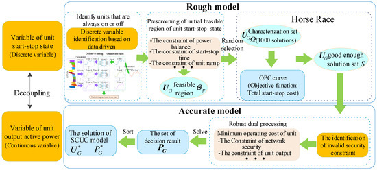
Figure 1. The overall idea of the improved constrained order optimization (COO) algorithm.

Step 1. First, the SCUC discrete variable identification model for the start–stop state of the units is constructed based on the deep learning idea, and the constant units are identified in discrete variable space. Then, the initial feasible region of the start–stop state (U_Git) is formed by eliminating the constant units. Moreover, the SCUC model is decoupled, and the variable U_Git is taken to construct a COO rough model with its related constraints and start–stop cost. The initial feasible region of the start–stop state of the units is prescreened, and the feasible region Θ_N is obtained. Select N feasible solutions from feasible region Θ_N according to a uniform distribution to form a characterization set Ω. The number of N is closely related to the size of the solution space. Reference [19] showed that the number of N is generally 1000, as the solution space is less than 10⁸.

Step 2. Z solutions are selected further from the characterization set Ω as the selected set S based on the Horse Race method [11,20]. In set S, it must be guaranteed that at least α% of the probability contains k good enough solutions. The specific selection rule of the Horse Race method is as follows.

Firstly, the COO rough model is utilized to evaluate and sort the solutions in the characterization set Ω, and the order performance curve (OPC) is formed. Secondly, the type of OPC curve generated is determined based on the standard OPC curve. Thirdly, the optimization parameter in equation (6) [20] is determined according to the type of the OPC, and the value of Z is obtained. Finally, the previous Z solutions are selected from the sorted characterization set Ω to form the selected set S. The Z solution model is as follows.

$$Z\left(k,g\right)=e^{Z_0}·k^{\rho }·g^{\gamma }+\eta$$

(16)

The meanings of all the symbols in (16) are shown in [20].

Step 3. The identification model of the invalid security constraints is constructed first to eliminate the invalid security constraints. Second, the minimum total cost of units is taken as an objective function. Then, a COO accurate model of continuous variable P_Git is constructed under the condition of considering the constraints related to the active power output. Solving the unit output scheme and operation cost corresponding to the unit start–stop state in selected set S. Finally, the COO accurate model is employed to sort the set S to obtain the optimal solution.

4. Improved Strategy for the COO Algorithm

4.1. Improved Strategy for the COO Rough Model

The key to ensuring the efficiency and accuracy of the COO algorithm is to construct a reasonable COO rough model. The solution of the COO rough model needs to be simpler than that of the COO accurate model to ensure the rapid prescreening of the solution space. In addition, the COO rough model should be able to reflect the relative merits and demerits of the solutions accurately to preliminarily sort the solution space.

Some constant units during the short time scale of day-ahead scheduling are affected by the load level and the installed capacity of the system. Therefore, the computational efficiency of the COO rough model can be improved greatly if the constant units before the COO rough model are screened. A novel data-driven SCUC discrete variable identification method is first proposed in this paper to improve the COO rough model.

4.1.1. The Data-Driven SCUC Discrete Variable Identification Strategy

A deep learning model is constructed by using Long Short-Term Memory (LSTM), which can accept the input of a time series structure. The mapping relationship of deep learning between the system load and the start–stop state of the units is created through massive historical data training. Based on the deep learning model, the constant units are identified.

In the real power system, the similarity of the daily load curve is relatively higher in the short period and in the same period each year. However, the load curve varies sharply in different months and seasons due to environmental and climatic factors. These historical data will easily lead to overfitting and reduce the calculation accuracy if they are directly used to train the deep learning model without distinction. Thus, it is necessary to preprocess the historical data by clustering and constructing a deep learning model for each type of historical data. The type of load data input is first determined, and then, the corresponding mapping model is used to solve the problem as the decision-making step. The process is shown in Figure 2. The structure of the deep learning model based on LSTM is shown in Figure 3.

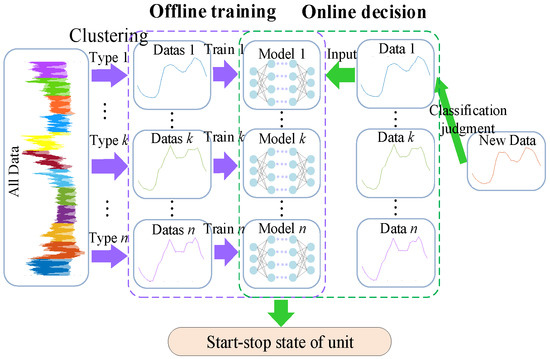
Figure 2. Deep learning model for the discrete variable identification.

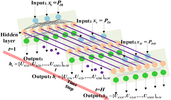
Figure 3. The structure of the deep learning model.

The parameter x_t represents the load data input to the deep learning model at time t in Figure 3, and x_t is equal to P_Dt. The symbol h_t is the start–stop state vector of all units output by the deep learning model at time t, and h_t equals [U_G1t,U_G2t,…,U_GMt]_1×M. The total number of units is M. The hidden layer is composed of LSTM neurons. Its depth is set after the size of data input, the structure factors, and the training test results are all considered. The training process of the deep learning model can be found in [21].

The internal structure of the LSTM neuron is shown in Figure 4.

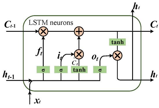
Figure 4. Internal structure of using Long Short-Term Memory (LSTM) neuron.

Combined with historical sample data of SCUC, mathematical models of the LSTM neuron are constructed as follows.

$$\{\begin{array}{l}{f}_t=\mathbf{\sigma }(W_f·[P_{Dt},[U_{G1t},U_{G2t},\dots ,U_{GMt}]]+b_f)\\ i_t=\mathbf{\sigma }(W_i·[P_{Dt},[U_{G1t-1},U_{G2t-1},\dots ,U_{GMt-1}]]+b_i)\\ {\tilde{C}}_t=\mathit{tanh}(W_C·[P_{Dt},[U_{G1t-1},U_{G2t-1},\dots ,U_{GMt-1}]]+b_C)\\ o_t=\mathbf{\sigma }(W_o·[P_{Dt},[U_{G1t-1},U_{G2t-1},\dots ,U_{GMt-1}]]+b_o)\\ [U_{G1t},U_{G2t},\dots ,U_{GMt}]=\mathit{tanh}(W_h·C_t+b_h)·o_t\\ C_t=f_t\ast C_{t-1}+i_t\ast {\tilde{C}}_t\end{array}$$

(17)

where “·” represents the element multiplication in the matrix. “*” represents matrix multiplication. W_f, W_i, W_C, W_o, W_h represents the weight value of the input parameter. b_f, b_i, b_C, b_o, b_h represents the offset value of each input parameter. A detailed description of the symbols can be found in [14].

4.1.2. Construction and Solution of the COO Rough Model

The COO rough model is constructed according to the constraints related to the start–stop state variables U_Git. The main constraints include the power balance constraint, unit climbing constraint, and minimum start–stop time constraint. The mathematical model is shown in (18).

$$\{\begin{array}{l}{\displaystyle \sum _{i=1}^M{U}_{Git}·P_{Gi\max }+{\displaystyle \sum _{j=1}^W{P}_{Wjt}}\ge P_{Dt}}+\Delta P_{Dt}\\ {\displaystyle \sum _{i=1}^M{U}_{Git}·P_{Gi\min }+{\displaystyle \sum _{j=1}^W{P}_{Wjt}}\le P_{Dt}}\\ {\displaystyle \sum _{t=1}^T\left|U_{Git}-U_{Gi(t-1)}\right|}\le n_i\\ {\displaystyle \sum _{t’=t+2}^{t+MU{T}_{Gi}}(1-U_{Gi{t}^{’}})}+MU{T}_{Gi}·\left(U_{Git}-U_{Gi(t-1)}\right)\le MU{T}_{Gi}\\ {\displaystyle \sum _{t’=t+2}^{t+MD{T}_{Gi}}{U}_{Gi{t}^{’}}}+MD{T}_{Gi}·\left(U_{Gi(t-1)}-U_{Git}\right)\le MD{T}_{Gi}\\ {\displaystyle \sum _{i=1}^M\left[\Delta P_{Gi}^{up}·U_{Git}+P_{Gi\min }·(U_{Git}-U_{Gi(t-1)})\right]\ge P_{Dt}-P_{D(t-1)}}\\ {\displaystyle \sum _{i=1}^M\left[\Delta P_{Gi}^{down}·U_{Git-1}+P_{Gi\min }·(U_{Gi(t-1)}-U_{Git})\right]\ge P_{D(t-1)}-P_{Dt}}\end{array}$$

(18)

where ΔP_Dt represents the active power reserved by the system at time t.

First, the data-driven SCUC discrete variable identification strategy is utilized to determine constant units. Then, equation (18) is used to screen the solution space, and the feasible region Θ_N of unit start–stop variable U_Git can be obtained. The N feasible solutions are selected randomly and uniformly in the feasible region Θ_N, and the cost F₁ for all start–stop units is taken as the objective function. Meanwhile, the OPC is drawn, and the set S of unit start–stop variable U_Git is sequenced further. The objective function is shown in (19).

$$F_1={\displaystyle \sum _{t=1}^H{\displaystyle \sum _{i=1}^M{U}_{Git}·(1-U_{Gi(t-1)})·S_{Git}\left({\tau }_{ti}\right)}}$$

(19)

4.2. Improved Strategy for the COO Accurate Model

The scale of modern power systems is huge, and there are many nodes. Therefore, solving the equation of power flow and checking network security constraints are some of the most time-consuming parts in the process of solving SCUC problems. Only a small part of the constraints is effective, which could restrict the formation of the feasible region among all the network security constraints shown in [17]. From this viewpoint, the invalid security constraints identification strategy is introduced first, and the accurate COO model is improved on this basis.

4.2.1. The Invalid Security Constraints Identification Strategy

The invalid constraint is defined as follows. The constraint is an invalid constraint if the feasible region is the same, no matter if the constraint is removed or not. The principle is shown in Figure 5.

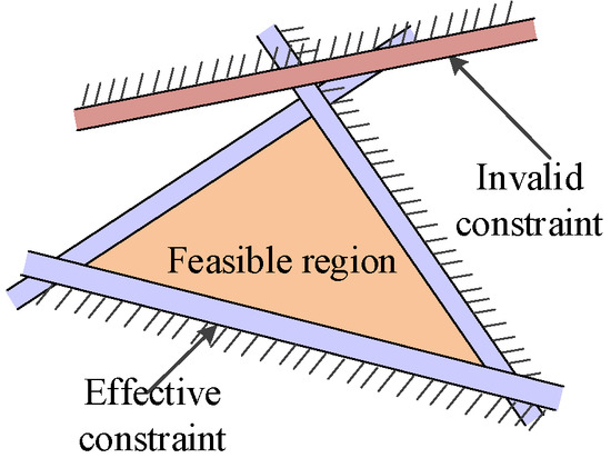
Figure 5. Definition of the invalid constraint.

The network security constraint condition of the power system, which is a bilateral constraint, is shown in (15). The bilateral constraint condition can be judged as an invalid constraint if both unilateral constraints in (15) are invalid constraints. The bilateral constraints in (15) are divided into the unilateral constraints in (20):

$$\begin{array}{l}{\displaystyle \sum _{i=1}^M(K_{Gli}·P_{Git})}+{\displaystyle \sum _{j=1}^W(K_{Wlj}·P_{Wjt})}-{\displaystyle \sum _{k=1}^D(K_{Dlk}·P_{Dkt})}\le P_{l\max }\\ {\displaystyle \sum _{i=1}^M(K_{Gli}·P_{Git})}+{\displaystyle \sum _{j=1}^W(K_{Wlj}·P_{Wjt})}-{\displaystyle \sum _{k=1}^D(K_{Dlk}·P_{Dkt})}\ge -P_{l\max }\end{array}$$

(20)

Two identification models with the unilateral invalid constraints are established according to (20).

$$\underset{P_{Git},P_{Wjt}}{\mathit{min}}{\mathit{L}}_l^{+}={\displaystyle \sum _{i=1}^M(K_{Gli}·P_{Git})}+{\displaystyle \sum _{j=1}^W(K_{Wlj}·P_{Wjt})}-{\displaystyle \sum _{k=1}^D(K_{Dlk}·P_{Dkt})}$$

(21)

$$\underset{P_{Git},P_{Wjt}}{\mathit{min}}{\mathit{L}}_l^{-}=-{\displaystyle \sum _{i=1}^M(K_{Gli}·P_{Git})}-{\displaystyle \sum _{j=1}^W(K_{Wlj}·P_{Wjt})}+{\displaystyle \sum _{k=1}^D(K_{Dlk}·P_{Dkt})}$$

(22)

$$P_{Gi\min }\le P_{Git}\le P_{Gi\max }$$

(23)

$$P_{Wjt}{}^{-}\le P_{Wjt}\le P_{Wjt}{}^{+}$$

(24)

The minimum ${\mathit{L}}_l^{+}$ is solved by (21), (23), and (24). The minimum ${\mathit{L}}_l^{-}$ is also solved by (22)–(24). It indicates that the l^th security constraint is invalid if both ${\mathit{L}}_l^{+}\ge -P_{l\max }$ and ${\mathit{L}}_l^{-}\ge -P_{l\max }$ satisfy the conditions.

4.2.2. Construction and Solution of the COO Accurate Model

The COO accurate model is constructed based on the invalid security constraints identification strategy. The COO accurate model sets the unit output P_Git as the variable and takes the systems start–stop costs and operation costs as the objective function. Meanwhile, the set S is evaluated accurately to obtain the optimal solution. The variable U_Git is a constant for the COO accurate model, and the corresponding start–stop cost F₁ is also a constant. Therefore, the decision variables are only P_Git in the COO accurate model. The COO accurate model is shown in (25) to minimize the total SCUC cost.

Equation (25) is a min–max model that cannot be solved directly. Thus, dual transformation is first needed to process it. Equation (25) is the linear objective function and the constraint condition of the uncertain variable P_W for the inner max model. Therefore, the duality model of the inner model is directly obtained according to the linear duality theorem. Combining the outer max model, the final form (26) of the dual transformation model is obtained.

$$\begin{array}{l}F(P_G)={\displaystyle \sum _{t=1}^H{\displaystyle \sum _{i=1}^M\left\{\underset{P_G}{\mathit{min}}\underset{P_W\in [P_W{}^{-},P_W{}^{+}]}{\mathit{max}}\left[(a_i+b_i·P_{Git}+c_i·P_{Git}{}^2)+F_1\right]\right\}}}\\ \{\begin{array}{l}{U}_{Git}·P_{Gi\min }\le P_{Git}\le U_{Git}·P_{Gi\max }\\ {\displaystyle \sum _{i=1}^M{U}_{Git}·P_{Git}+{\displaystyle \sum _{j=1}^W{P}_{Wjt}}=}{P}_{Dt}\\ {\displaystyle \sum _{i=1}^M\left[\Delta P_{Gi}^{up}·U_{Git}+P_{Gi\min }·(U_{Git}-U_{Gi(t-1)})\right]\ge {\displaystyle \sum _{i=1}^M{P}_{Git}-P_{Gi(t-1)}}}\\ {\displaystyle \sum _{i=1}^M\left[\Delta P_{Gi}^{down}·U_{Git-1}+P_{Gi\min }·(U_{Gi(t-1)}-U_{Git})\right]\ge {\displaystyle \sum _{i=1}^M{P}_{Gi(t-1)}-P_{Git}}}\\ -P_{l\max }\le {\mathit{P}}_{\mathit{l}}^{(l)}\le P_{l\max }\end{array}\end{array}$$

(25)

where P_l^(l) represents the active power on the remaining line after removing the invalid constraint on the line l.

$$\begin{array}{l}\underset{P_G,\lambda }{\mathit{min}}g(P_G,\lambda )\\ st.\{\begin{array}{l}{\phi }_1(P_G,\lambda )=0\\ {\phi }_2(P_G)\le 0\\ {\phi }_3(P_G,\lambda )\le 0\end{array}\end{array}$$

(26)

where P_G represents the matrix of active power output from thermal power units. λ represents the dual variable of the P_W. φ₁ represents the equation constraints containing P_G and P_W. φ₂ represents the inequality constraint containing only P_G. φ₃ represents the inequality constraints containing P_G and P_W.

5. Numerical Simulation

5.1. The Test System

The numerical tests are performed on a modified IEEE 118-bus system, which includes 54 thermal units, 91 demand sides, and 3 wind farms. The three wind farms in which the rated powers are 100, 200, and 250 MW, are accessed at the bus 14, 54, and 95, respectively. The load data is based on the actual load data of 365 typical days in a certain area of Hunan Province in 2014, and it is reduced by 4.4 times. The scheduling period is H = 24 h. The related calculations are done on the Intel Core i5-7500 processor 3.40 GHz, 8G memory computer. The improved COO algorithm in this paper is implemented using Matlab 9.0 and CPLEX 12.4, but the discrete variable identification process is implemented in the Python 3.6 environment.

In this paper, the training and test sample data in the deep learning model are generated by using the decision-making method in [9]. The above data are calculated based on load data from the Hunan power grid. The load data are divided into four types by cluster analysis. Under each type, 6% of the data are selected randomly as the test data, and the remaining 94% are left as training data. The size of the training and test samples is shown in Table 1.

Table 1. Sample size.

Type of Samples	1	2	3	4
Number of training samples	86	74	125	58
Number of test samples	86	74	125	58

5.2. SCUC Decision Process and Results based on the Improved COO Algorithm

The specific solving process in the improved COO algorithm is analyzed by taking the first test sample in the beginning type of data as an example. The load data of the test sample and the predicted expected value for the wind power output are shown in Table A1 of the Appendix A.

The COO rough model is used to calculate and form the feasible region Θ_N. Then, a method of simple random sampling is used to select 1000 solution sets from the feasible region Θ_N to form the characterization set Ω. The start–stop cost corresponding to each feasible solution is solved according to (19). The OPC is shown in Figure 6.

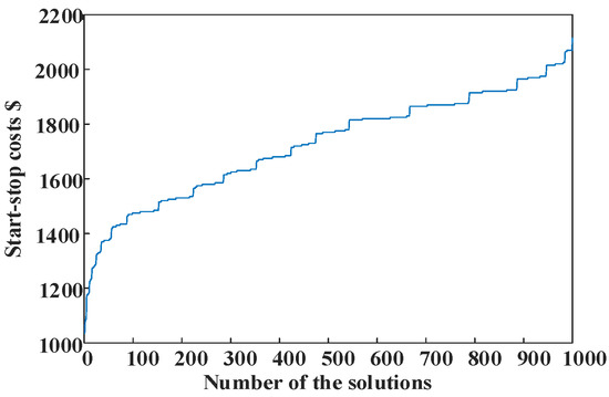
Figure 6. The OPC of solutions.

The OPC in Figure 6 is stepped because the start–stop costs of different units may be the same under different start–stop schemes. The OPC type obtained by the improved COO algorithm is determined to be bell-shaped compared with the standard curve of the OPC in [20]. The probability that at least one solution from the set S belongs to the accurate solution set of the original problem is set to 95%. The parameters in (17) are determined as follows: Z₀ = 8.1998, ρ = 1.9164, γ = –2.0250, η = 10, g = 20, and k = 1 according to [20]. The above parameters are substituted into (16), and the solutions number in the set S is 19. The COO accurate model solves the set S accurately of the COO rough model, and the results are shown in Figure 7.

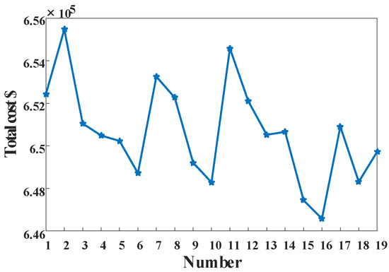
Figure 7. The results of the COO accurate model.

The start–stop and output scheme (No. 16) with the lowest total cost is selected as the decision result. In this study, the output scheme of each unit is shown in Table A2 of the Appendix A.

5.3. Validation of the Improved COO Rough Model

Compared with [16], the effectiveness of the discrete variable identification method in this paper is verified. Compared with the traditional COO rough model [12], the effectiveness of the improved COO rough model is verified.

5.3.1. Effectiveness of the Discrete Variable Identification Method

The SCUC training sample data are utilized for training the LSTM-based deep learning model in this paper. The network parameters of the constructed deep learning model are shown in Table 2.

Table 2. Parameter of the deep learning model.

Type of Samples	1	2	3	4
Number of hidden layers	4
Number of single-layer neurons in the hidden layer	256	256	256	256
Batch size	8	8	8	4
Learning rate	0.001
Optimization solver	Adam
Epochs	500	500	800	600

Figure 8 shows that the training error in the deep learning model decreases as the number of training increases for each type of training sample. In other words, the constructed deep learning model proposed in this paper converges.

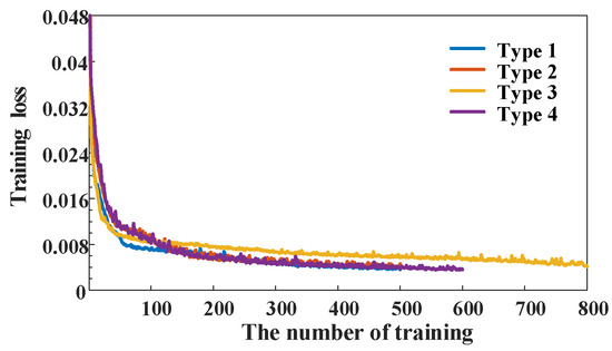
Figure 8. Training error of the deep learning model.

The discrete variable identification results based on the clustered data of load test samples, and the identification results are compared with real start–stop state data. The Precision and Recall evaluation indexes are used to verify the correctness of the data-driven discrete variable identification strategy. The specific calculation of Precision and Recall are as follows.

$$PRE=\frac{TP}{TP+FP}$$

(27)

$$REC=\frac{TP}{TP+FN}$$

(28)

where PRE represents Precision. REC represents Recall_. TP represents among the units that have been identified, the number of correct identification units. FP represents among the units that have been identified, the number of units that are misidentified. FN represents among the units that have been identified, the number of units that should have been identified but missing.

A Precision of 100% means that the identification results are all correct, and there is no erroneous recognition unit. A Recall of 100% indicates that the identified results are all correct, and there is no missing unit. The COO algorithm can correct the missing units in the COO accurate model stage. Nevertheless, it has no ability to correct incorrect identification units. Thus, the discrete variable identification model must guarantee a Precision of 100%, and the higher the Recall is, the better it is. However, a Recall of 100% is not mandatory.

As seen in Figure 9, the Precision is 100%. It is the same as the method in [16] for all samples. This result indicates that there is no error identification result. The Recall in the proposed algorithm is higher than that in [16], which means that it can greatly improve the Recall of the unit start–stop states under the condition of ensuring no error identification.

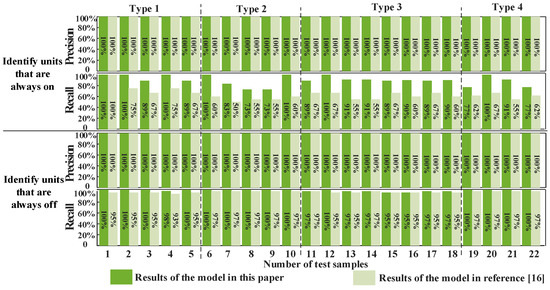
Figure 9. Comparison diagram of the discrete variable identification results.

Compared with the real unit output, it is found that the active power output value of some units in the scheduling scheme solved by this method fluctuates sharply. Therefore, reference [16] set the identification rate parameter directly through subjective judgment, which is not enough to identify as many constant units as possible. Consequently, the Recall is relatively higher. The method of this paper uses the massive historical data to train the deep learning model, and creates the mapping relationship between the load and the constant units directly, which has a stronger objectivity and a higher accuracy.

Comparing the computational time of the COO rough model with that of [16], the results of each test sample are shown in Table 3.

Table 3. Comparison of the discrete variable identification efficiency.

Number of Test Samples	1	2	3	4	5	6	7	8	9	10	11
Improved COO/s	0.22	0.25	0.22	0.21	0.21	0.21	0.20	0.21	0.23	0.21	0.25
Reference [16]/s	3.72	2.36	2.39	2.40	1.54	1.65	1.33	1.69	1.69	1.73	1.83
Number of test samples	12	13	14	15	16	17	18	19	20	21	22
Improved COO/s	0.27	0.24	0.26	0.24	0.28	0.25	0.28	0.17	0.18	0.17	0.17
Reference [16]/s	2.35	1.77	1.56	1.66	1.68	1.69	1.70	1.70	1.64	1.67	1.73

Table 3 shows that the computational efficiency of the discrete variable identification method is generally 0.2 seconds for 22 test samples, while the reference [16] is generally 2 seconds. The computational efficiency is improved by approximately 10 times compared with that in [16]. The reason is that the discrete variable identification method in [16] is essentially designed to solve the SCUC model, so the computational efficiency is lower. The proposed discrete variable identification method does not need to solve any optimization model. Instead, the method directly identifies the corresponding constant units according to the load data and the corresponding mapping relationship. The main reason is that the data-driven strategy of offline training and online decision-making is adopted. Thus, the calculation efficiency of this method is higher.

5.3.2. Effectiveness of the Improved COO Rough Model

Comparing the computational time of the COO rough model with that of the traditional COO rough model [12]. The results of each test sample are shown in Table 4.

Table 4. Comparison of computational efficiency of the COO rough model.

Number of Test Samples	1	2	3	4	5	6	7	8	9	10	11
Improved COO/s	12.79	3.19	3.65	2.49	3.63	14.94	4.15	22.62	45.49	12.44	7.01
Traditional COO [12]/s	588.27	59.21	60.81	35.99	82.40	786.22	254.11	208.13	492.96	470.86	237.81
Number of test samples	12	13	14	15	16	17	18	19	20	21	22
Improved COO/s	2.98	3.35	3.82	5.35	3.58	7.56	7.11	2.21	2.49	1.82	3.56
Traditional COO [12]/s	84.71	842.83	120.20	145.72	205.36	141.39	490.73	54.26	23.31	48.85	132.52

Table 4 shows that in 22 test samples, the computational efficiency of the improved COO rough model has a minimum improvement of approximately nine times, a maximum improvement of approximately 250 times, and an average improvement of approximately 40 times compared with the traditional COO rough model [12]. The reason is that the discrete variable identification method can reduce the dimension of the solution space effectively so that the computational efficiency of the COO rough model is improved as a whole.

5.4. Validation of the Improved COO Accurate Model

Firstly, the effectiveness of the invalid security constraints identification method is verified. Then the computational efficiency of the improved COO accurate model is compared with that of the traditional COO accurate model [12].

5.4.1. Effectiveness of the Invalid Safety Constraint Identification Method

Equations (20)–(24) are used to reduce the invalid security constraints. The number of remaining security constraints after reduction and the time consumed are shown in Table 5 for each test sample.

Table 5. Identification effect and efficiency comparison of the invalid security constraints model.

Number of Test Samples		1	2	3	4	5	6	7	8	9	10	11
Improved COO	Number of security constraints	432	192	192	432	192	240	240	384	240	432	192
	Time consuming/s	49.79	48.71	43.53	45.45	42.01	45.28	46.73	47.94	40.40	48.66	46.25
Traditional COO [12]	Number of security constraints	8928
	Time consuming/s	-
Number of Test Samples		12	13	14	15	16	17	18	19	20	21	22
Improved COO	Number of security constraints	192	192	192	192	192	192	240	240	240	240	240
	Time consuming/s	42.75	44.63	43.93	46.32	46.15	48.58	44.66	47.98	43.75	45.26	40.99
Traditional COO [12]	Number of security constraints	8928
	Time consuming/s	-

Table 5 shows that the number of invalid safety constraints is different for the different test samples. The reason is that the identification effect in the invalid safety constraints identification model is closely related to the load characteristics of each sample. Generally, the proposed strategy can reduce more than 90% of the invalid security constraints, and the time consumed is approximately 50 seconds, which indicates that the security constraints of the SCUC model may be redundant for real power systems. Thus, the identification strategy of invalid security constraints can eliminate redundant information quickly and effectively.

5.4.2. Effectiveness of the Improved COO Accurate Model

Comparing the computational time of the COO accurate model with that of the traditional COO accurate model [12]. The results of each test sample are shown in Table 6.

Table 6. Comparison of computational efficiency of the COO accurate model.

Number of Test Samples	1	2	3	4	5	6	7	8	9	10	11
Improved COO/s	979.35	945.78	851.54	906.03	832.40	890.34	922.55	994.06	819.38	990.31	909.98
Traditional COO [12]/s	4520.71	4516.04	4518.70	4544.77	4551.97	4526.56	4539.23	4525.08	4522.95	4521.71	4534.37
Number of test samples	12	13	14	15	16	17	18	19	20	21	22
Improved COO/s	845.97	890.27	885.47	926.87	927.82	969.90	901.84	943.53	867.22	905.66	832.63
Traditional COO [12]/s	4541.56	4549.07	4545.29	4522.92	4544.84	4529.94	4546.73	4536.00	4531.52	4535.02	4530.58

The computational efficiency of the improved COO accurate model has a minimum improvement of approximately 1.08 times, a maximum improvement of approximately 1.49 times, and an average improvement of approximately 1.28 times compared to the COO accurate model [12]. The main reason is that the invalid security constraints identification strategy is added to the COO accurate model, which can reduce the number of security constraints that need to be checked greatly. Thus, the computational efficiency of the COO accurate model is improved overall.

5.5. The Overall Validation of the Improved COO Algorithm

All 22 test samples are taken as examples in this paper, and the results are compared with those for the traditional COO algorithm [12] and algorithm [9] to verify the effectiveness of the improved COO algorithm. The comparison is shown in Table 7.

Table 7. Comparison of the solution results.

Number of Test Samples		1	2	3	4	5	6	7	8
Time consuming/s	Improved COO	992.14	948.97	855.19	908.52	836.03	905.28	926.70	1016.68
	Traditional COO [12]	5108.98	4575.25	4579.51	4580.76	4634.37	5312.78	4793.34	4733.21
	Reference [9]	6853.89	5725.86	5766.73	6628.94	6670.58	6554.07	6942.19	5960.24
Total cost/$	Improved COO	646567.97	723287.12	735334.93	681851.92	736779.38	904205.29	881413.65	892721.43
	Traditional COO [12]	762084.95	834375.86	844551.57	785415.66	849900.30	1012410.15	1007753.63	1005503.06
	Reference [9]	643344.97	721176.04	734184.82	680173.19	734196.97	899599.46	879674.38	886279.05
Number of Test Samples		9	10	11	12	13	14	15	16
Time consuming/s	Improved COO	864.87	1002.75	916.99	848.95	893.62	889.29	932.22	931.40
	Traditional COO [12]	5015.91	4992.57	4772.18	4626.27	5391.9	4665.49	4668.64	4750.2
	Reference [9]	5918.07	6939.63	5632.61	4977.96	6690.73	53529.03	5005.34	4925.83
Total cost/$	Improved COO	895247.17	909067.83	807019.64	745048.53	792798.54	815786.29	784518.73	795341.57
	Traditional COO [12]	1002927.66	1019975.26	920721.65	852746.32	914055.57	912394.40	888309.16	907311.33
	Reference [9]	887989.75	903668.74	802671.06	743535.53	790766.92	813371.25	779768.85	792900.62
Number of Test Samples		17	18	19	20	21	22
Time consuming/s	Improved COO	977.46	908.95	945.74	869.71	907.48	836.19
	Traditional COO [12]	4671.33	5037.46	4590.26	4554.83	4583.87	4663.1
	Reference [9]	5483.08	7268.37	5258.93	5614.96	5185.65	5388.78
Total cost/$	Improved COO	769253.58	829647.60	1025047.44	964064.70	990313.80	1066270.58
	Traditional COO [12]	873774.82	940060.80	1119787.68	1055604.58	1087159.16	1154272.57
	Reference [9]	766214.25	826838.02	1020704.11	958273.58	985874.15	1059706.18

It can be observed that the SCUC total cost solved in the improved COO algorithm is slightly higher than that in [9], while the total cost in the traditional COO [12] algorithm is the highest in Table 8. The SCUC total cost solved by the two COO algorithms is higher. The average solution precision of the proposed method is about 99.6%, while the traditional COO method is about 88.1%. Compared with the traditional COO method, the accuracy of the proposed method is 1.13 times higher. The main reason is that the COO algorithm is designed to improve the algorithm efficiency greatly by abandoning the search for the optimal solution and instead searching for a good enough solution. The SCUC total cost obtained by the improved COO algorithm is slightly lower than that in the traditional COO algorithm [12]. The reason is that the set S in the improved COO algorithm is not the same as that in the traditional COO screening. This improved COO reduces the dimension of the solution space through a discrete variable identification strategy so as to improve the quality of effective solutions. Therefore, the solution quality of the set S obtained by the improved COO algorithm is higher than the traditional COO algorithm.

Table 8. Robust and non-robust security-constrained unit commitment (SCUC) model.

Number of Test Samples		1	2	3	4	5	6	7	8
Time consuming/s	Robust optimization	992.14	948.97	855.19	908.52	836.03	905.28	926.70	1016.68
	Non-robust optimization	842.72	817.34	765.28	796.34	782.66	831.61	834.87	873.92
Total cost/$	Robust optimization	646567.97	723287.12	735334.93	681851.92	736779.38	904205.29	881413.65	892721.43
	Non-robust optimization	644868.75	721605.01	733495.09	680149.41	735101.31	901726.01	879236.15	890509.40
The number of lines over the active power limit	Robust optimization	0
	Non-robust optimization	12	12	11	13	12	15	13	15
Number of Test Samples		9	10	11	12	13	14	15	16
Time consuming/s	Robust optimization	864.87	1002.75	916.99	848.95	893.62	889.29	932.22	931.40
	Non-robust optimization	748.52	877.85	824.26	740.01	757.09	781.08	845.78	839.61
Total cost/$	Robust optimization	895247.17	909067.83	807019.64	745048.53	792798.54	815786.29	784518.73	795341.57
	Non-robust optimization	892841.17	906715.44	804717.21	742914.86	790764.82	813810.09	782710.63	793100.03
The number of lines over the active power limit	Robust optimization	0
	Non-robust optimization	14	17	12	11	11	13	13	12
Number of Test Samples		17	18	19	20	21	22
Time consuming/s	Robust optimization	977.46	908.95	945.74	869.71	907.48	836.19
	Non-robust optimization	841.78	802.45	816.69	733.93	773.88	731.15
Total cost/$	Robust optimization	769253.58	829647.60	1025047.44	964064.70	990313.80	1066270.58
	Non-robust optimization	767307.15	827476.31	1022080.75	961437.47	987522.98	1063575.53
The number of lines over the active power limit	Robust optimization	0
	Non-robust optimization	12	13	16	14	14	15

The efficiency of the improved COO algorithm has been improved significantly in terms of solving efficiency compared with the other two algorithms. The efficiency of the improved COO algorithm is approximately five times higher than that of the traditional COO [12] algorithm. It is also six times higher than that in [9]. There are two main reasons. The discrete variable identification strategy is introduced into the COO rough model, which reduces the dimension of the solution space effectively and improves the computational efficiency greatly. In addition, the invalid security constraints identification strategy is introduced in the COO accurate model, which eliminates the invalid security constraints and reduces the number of security constraints that need to be checked greatly. Thus, the computational efficiency is sharply improved.

5.6. Validation of the SCUC Model Considering the Uncertainty of Wind Power Output

In order to analyze the influence of wind power uncertainty on power system scheduling, the SCUC problem is solved with the proposed method under the two situations of considering wind power uncertainty and not considering wind power uncertainty. In this paper, the robust optimization method is used to deal with the uncertainty of wind power output. The scheduling cost, calculation efficiency, and over-limited power flow under two different situations of robust optimization and non-robust optimization are shown in Table 8.

It can be seen from Table 8 that the scheduling cost considering the uncertainty of wind power is higher than that not considering the uncertainty of wind power. The reason is that the SCUC decision based on the robust optimization method is to solve the thermal power unit scheduling scheme under the worst scenario of wind power output. The scheme is a conservative uncertainty factor processing method, so the cost is high. Considering the uncertainty of wind power, the calculation efficiency is low. The reason is that the dual optimization process is added to the robust optimization model. The network power flow considering the uncertainty of wind power does not exceed the limit, while the network power flow not considering the uncertainty of wind power exceeds the limit. The reason is that the wind power output is uncertain, and the actual wind power output value is not necessarily equal to the predicted value. The generated scheduling scheme will not guarantee the network security in the worst scenario of actual wind power output if the uncertainty of wind power output is not considered.

On the whole, considering the uncertainty of wind power output, the scheduling cost increases slightly and the calculation efficiency decreases slightly. Nevertheless, the network security is improved.

6. Conclusions

An improved COO algorithm for solving the SCUC problem was proposed in this paper. The SCUC problem was solved rapidly and effectively considering the uncertainty of wind power output. Simulations based on the IEEE 118-bus example were executed. First, the data-driven discrete variable identification strategy was incorporated into the COO rough model, and then, the invalid security constraints identification strategy was incorporated into the COO accurate model. Finally, the improved COO algorithm combined the discrete variable identification with the invalid security constraint identification to make the uncertain SCUC decision. The conclusions are as follows.

(1) A deep learning model based on LSTM was constructed, and then a data-driven SCUC discrete variable identification strategy was proposed. This strategy was applicated to the COO rough model. The proposed improvement strategy can enhance the computational efficiency greatly of the rough COO model under the premise of ensuring the solution accuracy.

(2) The invalid security constraints identification strategy can identify more than 90% of the invalid security constraints in a short period of time. The strategy introduced to the COO accurate model can effectively reduce the computational redundancy of the COO accurate model and improve its computational efficiency.

(3) The data-driven SCUC discrete variable identification strategy and the invalid security constraint identification strategy were introduced based on the COO algorithm. These strategies effectively improved the compactness and the overall efficiency of the COO algorithm. Compared with the traditional COO, the accuracy and efficiency of the proposed method were improved by nearly 1.13 times and 5 times, respectively.

On the whole, the actual situation, which is common in the SCUC problem, was considered in the method of this paper. By reducing the complexity of the solution space and the model, the purpose of improving the accuracy and efficiency of the solution was achieved.

References

- Ye, H.; Wang, J.; Li, Z. MIP Reformulation for max-min problems in Two-stage robust SCUC. IEEE Trans. Power Syst. 2017, 32, 1237–1247. [Google Scholar] [CrossRef]
- Li, Z.; Ye, L.; Zhao, Y.; Song, X.; Teng, J.; Jin, J. Short-term wind power prediction based on extreme learning machine with error correction. Prot. Control Mod. Power Syst. 2017, 3, 95–100. [Google Scholar] [CrossRef]
- Ai, Q.; Fan, S.; Piao, L. Optimal scheduling strategy for virtual power plants based on credibility theory. Prot. Control Mod. Power Syst. 2016, 1, 1–8. [Google Scholar] [CrossRef]
- Abujarad, S.Y.; Mustafa, M.W.; Jamian, J.J. Recent approaches of unit commitment in the presence of intermittent renewable energy resources: A Review. Renew. Sustain. Energy Rev. 2017, 70, 215–223. [Google Scholar] [CrossRef]
- Zheng, Q.P.; Wang, J.; Liu, A.L. Stochastic optimization for unit commitment—A review. IEEE Trans. Power Syst. 2015, 30, 1913–1924. [Google Scholar] [CrossRef]
- Guan, X.; Song, C.; Ho, Y.C.; Zhao, Q. Constrained ordinal optimization—A feasibility model based approach. Discret. Event Dyn. Syst. 2006, 16, 279–299. [Google Scholar] [CrossRef]
- Yang, N.; Ye, D.; Zhou, Z.; Cui, J.; Chen, D.; Wang, X. Research on modelling and solution of stochastic SCUC under AC power flow constraints. IET Gener. Transm. Distrib. 2018, 12, 3618–3625. [Google Scholar]
- Alemany, J.; Kasprzyk, L.; Magnago, F. Effects of binary variables in mixed integer linear programming based unit commitment in large-scale electricity markets. Electr. Power Syst. Res. 2018, 160, 429–438. [Google Scholar] [CrossRef]
- Zhang, Z.; Chen, Y.; Liu, X.; Wang, W. Two-Stage robust Security-Constrained Unit Commitment model considering time autocorrelation of wind/load prediction error and outage contingency probability of units. IEEE Access 2019, 7, 25398–25408. [Google Scholar] [CrossRef]
- Zhang, Y.; Wang, J.; Zeng, B. Chance-constrained two-stage unit commitment under uncertain load and wind power output using bilinear benders decomposition. IEEE Trans. Power Syst. 2017, 32, 3637–3647. [Google Scholar] [CrossRef]
- Jia, Q.S.; Ho, Y.C.; Zhao, Q.C. Comparison of selection rules for ordinal optimization. Math. Comput. Model. 2006, 43, 1150–1171. [Google Scholar] [CrossRef]
- Wu, H.; Shahidehpour, M. Stochastic SCUC solution with variable wind energy using constrained ordinal optimization. IEEE Trans. Sustain. Energy 2014, 5, 379–388. [Google Scholar] [CrossRef]
- Ouyang, Z.; Shahidehpour, S.M. An intelligent dynamic programming for unit commitment application. IEEE Trans. Power Syst. 1991, 6, 1203–1209. [Google Scholar] [CrossRef]
- Wang, S.; Xu, X.; Kong, X.; Zheng, Y. Extended priority list and discrete heuristic search for multi-objective unit commitment. Int. Trans. Electr. Energy Syst. 2017, 28, e2486. [Google Scholar] [CrossRef]
- Shahbazitabar, M.; Abdi, H. A novel priority-based stochastic unit commitment considering renewable energy sources and parking lot cooperation. Energy 2018, 161, 308–324. [Google Scholar] [CrossRef]
- Wang, Y.; Xia, Q.; Kang, C.Q. Identification of the active integer variables in security constrained unit commitment. Proc. CSEE 2010, 30, 46–52. [Google Scholar]
- Zhai, Q.; Guan, X.; Cheng, J.; Wu, H. Fast identification of inactive security constraints in SCUC problems. IEEE Trans. Power Syst. 2010, 25, 1946–1954. [Google Scholar] [CrossRef]
- Berckmoes, B.; Molenberghs, G. Approximate central limit theorems. J. Probab. 2017, 31, 1590–1605. [Google Scholar] [CrossRef]
- Lee, L.H.; Lau, T.W.E.; Ho, Y.C. Explanation of goal softening in ordinal optimization. IEEE Trans. Autom. Control 1999, 44, 94–99. [Google Scholar] [CrossRef]
- Lau, T.W.E.; Ho, Y.C. Universal alignment probabilities and subset selection for ordinal optimization. J. Optim. Theory Appl. 1997, 93, 455–489. [Google Scholar] [CrossRef]
- Klaus, G.; Rupesh, K.S.; Jan Koutník, J.; Steunebrink, B.R.; Schmidhube, J. LSTM: A search space odyssey. IEEE Trans. Neural Netw. Learn. Syst. 2017, 28, 2222–2232. [Google Scholar]
© 2019 by the authors. Licensee MDPI, Basel, Switzerland. This article is an open access article distributed under the terms and conditions of the Creative Commons Attribution (CC BY) license (http://creativecommons.org/licenses/by/4.0/).