Abstract
In the last few years, the perspective of climate change, energy, competitiveness, and fuel consumption in the transportation sector has become one of the most significant public policy issues of our time. As different methods are being adapted into light-duty vehicles like engine downsizing, on the other hand, the increase in carbon emissions of heavy-duty trucks is becoming a major concern. Although previous researches have studied the methodology for selecting optimized turbocharger performance, still further investigation is needed to create a method for achieving the highest performance for a sequential axial turbocharger. Therefore, in this study, the design of a two-stage turbocharger system that consists of a radial turbine connected in series to an axial turbine is considered. The specific two-stage turbine was designed specifically and will be tested on a MAN 6.9 L diesel truck engine. With the engine already equipped with a radial type turbine, the newly designed two-stage turbine will be adapted to the engine to give more efficiency and power to it. Firstly, the modelling and simulation of the engine were done in Gt-Power, to achieve the same power and torque curves presented in the MAN engine specification sheet. Once that was achieved, the second task was to design and optimise a radial and axial turbine, which will form part of a two-stage system, through Computational Fluid Dynamics (CFD) analysis. Necessary data were gathered from the engine’s output conditions, for the ability to design the new turbo system. Lastly, the new turbine data were entered into the new two-stage turbo GT-Power model, and a comparison of the results was made. The CFD analysis, executed in ANSYS, for the radial turbine gave an 83.4% efficiency at 85,000 rpm, and for the axial turbine, the efficiency achieved was 81.74% at 78,500 rpm.
1. Introduction
Over the years, one of the main challenges in automation applications is how to increase the engine’s performance while keeping in mind the economic and emission constraints. The main engine performance upgrade is boosting, which increases the engine’s specific torque and power density to drive downsizing that can result in better fuel economy while keeping the dynamic performance. Additional demand for boosting also arises from emissions of carbon dioxide. In several countries and states, taxation of passenger cars is directly linked to the amount of carbon dioxide generated in a standard duty cycle. In response to this, manufacturers are reducing the size of their engines either permanently or for parts of the duty cycle.
Turbocharging has long been the most common technology used to boost diesel engines in passenger vehicles, highway trucks, and several other machines. Most gasoline engines, however, are still naturally aspirated today, though the market penetration for boosted engines is growing rapidly [1]. A turbocharger is a turbine-driven forced induction device that works by forcing extra air to the engine’s combustion chamber, which increases the efficiency and power output.
The new era of turbochargers are designed to be smaller, lighter, and efficient, and one of the essential aspects of turbocharging is to reduce the rotating inertia. Throughout this investigation, an advanced turbocharging project will be undertaken. It will involve the modelling and simulation of a diesel engine but also the design and numerical simulation of a radial and axial inflow turbocharger, which will form part of an in-series two-stage turbocharger system for a diesel engine. To summarize, the axial turbine will be working along with a second conventional radial turbine turbocharger.
Another aspect that is forcing manufacturers to reduce emissions is that the government in each country taxes cars regarding their emissions. Prices in the UK vary from 0 to 2000 pounds yearly [2].
Therefore, in this study, the design of an axial turbine, which forms part of a two-stage turbocharger (radial–axial), will be tested to confirm if it can have positive results regarding the reduction of emissions and inertia but also at the same time keep its high performance.
The overall aim of this work was to achieve better performance for automotive application by optimizing the turbocharger design selection. For this purpose, this study investigated the design of a two-stage turbocharger system, which included a radial and an axial turbine in series, for application in a heavy-duty diesel engine. In the first step, a two-stage (radial and axial) turbocharger was designed for a diesel engine. Following, the modelling and simulation of a diesel engine were considered in GT-Power. Finally, optimisation with computational fluid dynamics (CFD) was undertaken on both of the turbines. Moreover, from the gathered results, the most efficient turbine models were imported in GT-Power, where the results indicated the performance improvement obtained by this unique configuration of the two-stage turbocharging system.
2. The Use of Radial and Axial Turbochargers
Turbocharging has long been the standard technology used to boost diesel engines in passenger vehicles compared to the majority of gasoline engines; however, it is still aspirated today. Achieving higher exhaust gas temperatures in gasoline engines is desired and cost reduction is important simultaneously, but the main reason for choosing a turbocharger is that the air mass flow varies much more in a gasoline engine than in a diesel engine: A ratio of 80:1 from idle to rated power for a gasoline engine compared to just 6:1 in a passenger car diesel [3].
In the automotive industry, there are three main types of turbine designs available on the market: The conventional radial, the mixed-flow and the axial turbine. For turbocharging, there is also the option of mixed-flow turbines, but the present work will only deal with the two principal types. Axial turbines have been used as part of gas turbine powerplants for many industries, such as marine, aerospace, and industrial power generation, but the challenge for automotive application is how they can be adapted on vehicles. The radial turbine’s working principle is that the exhaust gas enters perpendicular to the rotor blades radially, and it is redirected 90° by the rotor before exiting the housing in the axial direction. On the other hand, axial turbines work in the opposite manner: The exhaust gas enters the rotor axially and exits in a radial direction. In an axial turbine, there is less mechanical stress on the blades due to the fact that the flow enters the turbine at a zero angle [4].
An example of the new era of turbochargers is the HTT dual boost turbocharger by Honeywell, which is the first time that an axial turbine has been utilized in the automotive sector. Three features have made Honeywell’s axial turbines unique: Zero-reaction aerodynamics, no nozzles, and tall-blade design. These three features have enabled the axial turbines to attain higher specific speeds, allowing a smaller size but with the same flow, resulting in the inertia being lowered by up to 40%. In addition, the axial turbines are designed for excellent efficiency under pulsating flows, and improve the catalyst light-off [2].
Another example of an axial turbine is Honeywell’s two-stage turbo system shown in Figure 1. It consists of a high-pressure turbocharger with a radial compressor and turbine wheels, joined with a low-pressure turbocharger consisting of a radial compressor wheel and an axial turbine stage. In a traditional radial/radial two-stage boosting system, exhaust gas must exit the high-pressure turbine, and makes a sharp bend into the low-pressure turbine. Given the high velocity of exhaust gas post-turbine and the degree of swirl left in the flow in off-design conditions, the total pressure drop in the inter-stage turbine duct results in a significant performance penalty [5].
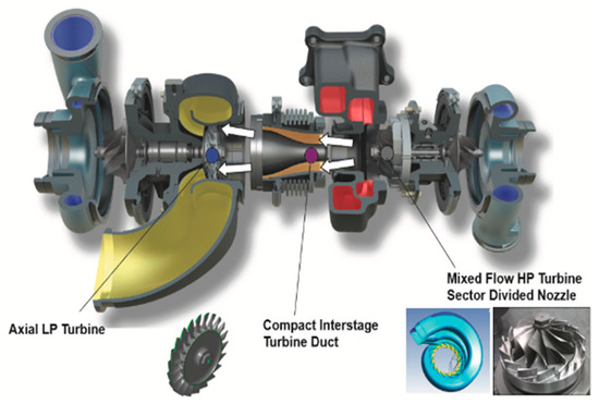
Figure 1.
Honeywell twin turbo system.
By using an axial low-pressure turbine stage mounted concentrically with the high-pressure stage, sharp bends between the stages are avoided.
Furthermore, due to the design of the duct and the low-pressure turbine, kinetic energy not recovered from the flow in the high-pressure stage can be converted into useful work by the low-pressure turbine stage. This integrated duct design gives the ability to have a compact, high-performance two-stage turbo system that is feasible to package in a modern vehicle chassis [5].
Two-stage serial system turbochargers consist of a small high-pressure turbo that works along with a larger low-pressure turbo. The gas flow between the turbos is controlled by by-pass valves, whose operation is based on the engine speed. At low speeds of up to about 1500 rpm, the two turbos work in full serial mode, with the compressor and turbine by-pass valves closed. This provides a rapid boost in pressure and contributes to enhanced torque and responsiveness. Beyond 1500 rpm, the turbos continue to work together, but the turbine by-pass valve progressively channels more exhaust gas to the larger low-pressure turbo until the full transition takes place, usually around 2800 rpm. At this speed, both the turbine and compressor by-pass valves are fully open, regulating the gas flow only to the larger low-pressure turbo [6].
The advantages of a two-stage system include having an excellent transient response, giving more power and torque, and maintaining fuel efficiency. Two-stage turbochargers have provided the ability for automotive industries to downsize larger engines but still maintain the same specifications. However, there are two main disadvantages of two-stage turbocharging. These are packaging and performance, as it is hard to be assembled in a modern vehicle, and the tight and complex bends result in a reduction of the performance. The inter-stage duct routing gases from the high-pressure turbine to the low-pressure turbine tend to be the highest loss component in the system [7].
Mixed-flow turbines, compared to radial inflow turbines, have the advantage of additional degrees of freedom for aero design due to radial turbines adopting mechanical constraints. The inlet blade angle of a mixed-flow turbine can be nonzero even with radial blade sections. With mixed-flow turbines, it is possible to gain more efficient results compared to radial turbines with respect to automotive applications. A characteristic that mixed flow turbines have is low inertia, which positively affects the transient response [8].
A reduction of the turbocharger’s rotating inertia will result in a significant improvement in the transient response of the turbocharger. The smaller the turbocharger, the lower the inertia; smaller turbochargers will provide more boost at lower speeds [9]. One approach to reducing the inertia is by improving the aerodynamic design, which reduces the number of blades without reducing turbine efficiency. Another method utilizes a lower inertia mixed-flow turbine rather than a radial flow turbine. Materials can also lower inertia by reducing their weight, for instance, by replacing the metal turbine rotor with a lower density ceramic one. Despite the high cost, titanium aluminium can be used and has been proven to help reduce inertia. The new technology of using an axial flow turbine rotor rather than the heavy radial inflow rotors can also result in the reduction of inertia [10].
Some turbochargers use precise bearings on their shaft made of advanced materials to handle the speed and temperature of the turbocharger. This type of bearing provides less friction than the fluid ones commonly used and allows a smaller, lighter shaft to be used [9].
Honeywell’s Dualboost aerodynamic design, which uses a double-sided compressor wheel in combination with an axial turbine, has made a significant change in the industry. It has equivalent overall efficiencies with competitors but much larger turbine efficiencies under low-speed unsteady conditions and up to 50% less rotating inertia [11].
Turbocharger lag is the most notable feature of diesel engine boosting. It is caused because the fuel pump responds rapidly to the increased fuelling demand after a load or speed increase. The engine air supply cannot match this higher fuel flow instantly but only after several engine cycles, owing to the inertia of the whole system. The above phenomenon is enhanced by unfavourable turbocharger compressor characteristics at low loads and speeds (Figure 2) [12].
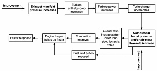
Figure 2.
Main mechanism of transient response improvement [12].
Turbochargers must be precisely matched to the engine’s fuel rate setting and engine displacement to achieve the correct boost pressure for the engine’s design points. This means every horsepower rating and torque rise profile in an engine family uses a uniquely sized turbocharger. On most engines, maximum boost pressure from the turbocharger will correspond to the engine’s peak-torque spot with minimal exhaust backpressure [13].
3. Turbine Preliminary Design
As part of the investigation on turbochargers, in-depth research on radial and axial turbines will be analysed to obtain an understanding of the design and essential aspects of turbines. This section includes concepts, such as rotor and blade design, and methods that will be followed in this study. The basic theory of the radial turbine will be described followed by the axial blade design theory.
For decades, the radial turbine has been the most used turbine, specifically in power system applications, due to the ability to extract large shaft work in situations with low mass flow rates [14].
The rotor in a turbine is described as the heart of the turbine that converts energy from gases and transfers it into the compressor. Figure 3 presents a schematic diagram of a radial turbine and its components.
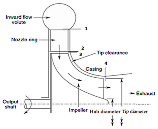
Figure 3.
Radial turbine components [15].
The equations shown below represent a non-dimensional volumetric flow rate and a total enthalpy drop (flow, Φ, and head coefficients, ψ, respectively); also by using an ideal gas assumption, the main dimensions of the rotor are determined [16]:
where ξ represents the ratio of the absolute velocities at the inlet and outlet of the rotor, and ε is the rotor (outlet and inlet) radius ratio. Velocity triangles at the inlet and the exit from the rotor blade can describe the characteristics of changes in the mass flow rate of various turbines. This statement is crucial in any turbine model, as all models must possess a similar or the same profile (velocity triangles) [17].
The main geometric characteristics of a typical radial inflow turbine, such as the radius, blade height, length, and throat openings, are displayed in Figure 4. The total and static pressure ratio can be calculated through the definition of the isentropic efficiency of the calorically perfect gas, as stated in Equation (3) assuming the conditions of Equation (4) are met:
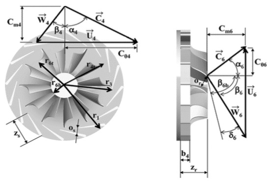
Figure 4.
Velocity triangles and radial inflow turbine geometric.
The number of blades can be calculated from the following equation [16]:
From Euler’s energy equation, the specific shaft work can be calculated from Equation (6) [14]:
Critical velocity is defined by:
The critical Mach number for the radial turbine can be defined as [14]:
Turbine-specific work is obtained by:
The efficiency can be found from Equation (10) [14]:
Throughout this section, the theory that has been applied for the design of axial turbines is explained. It starts from the velocity triangle theory and continues with the blade design method. The geometry of an axial blade can be described with different blade profiles and several angles. Moreover, a velocity diagram is an important tool in order to describe the velocity of the inlet fluid inside the turbine blades. The velocity diagram in Figure 5 represents the speeds and loads at which the working conditions of the blades will work [18].
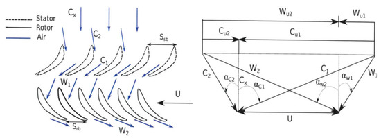
Figure 5.
Velocity diagram for axial turbine.
For the construction of a velocity triangle, the working parameters need to be specified. The loading coefficient is calculated with the following equation [18]:
The loading coefficient for turbines should always be positive. From Equation (11), the speed of the blade can be found if the change in enthalpy is known. By knowing the blade’s outer diameter from modelling software, and the relationship between speed and angular velocity, , the angular velocity can be calculated. The next step is to calculate the inlet velocity of the fluid by using the ideal gas law [18]:
and the volumetric flow becomes:
By knowing the inlet diameter Dp or assuming the value the air velocity can be calculated using:
and the flow coefficient of air can be calculated by:
For the next step, in order to calculate C1, C2, W1, and W2, the following relationships are used [18]:
Then, the angles for the flow passes are calculated using the following relationships:
After the process for the construction of the velocity triangles, the next step is the development of the blade profile for the stator and rotor of the turbine. Figure 6 shows the parameters for the development of the blade profile.
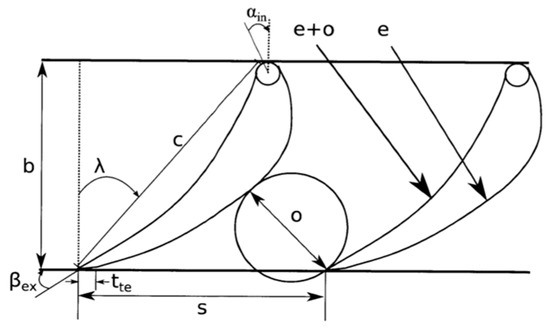
Figure 6.
Blade profile [18].
In the first step, the number of blades need to be determined for the stator and rotor. The number of blades for gas turbines vary between 11 and 110 blades. Usually, the blades for the stator are given as an odd number whereas the rotor blades have an even number to balance the weight. After the numbers of blades is chosen, the space between them can be found with the following equation:
Since the diameter is known and the number of blades has been chosen, the axial chord can be found from the following relationship:
The stagger angle is defined by the following equation:
The next step is to investigate a single stage configuration. By knowing the turbine inlet total conditions and the total pressure ratio and making an assumption of the efficiency, the exit turbine temperature can be calculated.
4. Design and Modelling Setup
This section will provide a concise and precise description of the experimental results, their interpretation as well as the experimental conclusions that can be drawn. As mentioned previously the goal of this study was the design of a two-stage turbocharger that consists of radial and axial turbine. It is a serial system with a radial turbine connected to an axial one. This configuration is relatively new in the automotive industry, and only Honeywell has attempted to use it.
The new designs of the turbines were created with the considerations to match a 6.9 L diesel engine for a MAN truck. The specific engine is equipped with a radial turbocharger, which will be replaced with the new two-stage one. A vital part of the study is the methodology as it clarifies the objectives of this investigation.
All the theories mentioned in the previous section are involved in this specific content. The following demonstrate the modelling approach details utilized in this research:
- Engine simulation and modelling;
- Radial blade design and setup (meshing, boundary conditions);
- Axial blade design and setup (meshing, boundary conditions);
- Blade optimisation;
- Map design;
- Two-stage turbocharger engine remodelled; and
- Final run.
A very significant factor in designing new turbochargers is the modelling and simulation of the engine that follows the turbo’s performance target. The working conditions of each turbocharger can have a massive effect on the performance and efficiency of the engine. Choosing the wrong turbocharger can lead to severe effects of turbo lag, an increase in fuel consumption, and a reduction in power and efficiency. Therefore, each turbocharger is designed based on specific engine characteristics.
The chosen software for the modelling of the engine was GT-Power due to it being the industrial standard of engine performance simulation used by several engine manufacturers and OEMs. It has capabilities, from performance quantities like power torque and turbocharger performance, to cylinder and tailpipe output emissions. To start, an in-depth research was done to choose the desirable engine as a case study for this study. After a critical review of previous research, the engine that was chosen was an MAN inline six cylinder 6.9 L diesel engine, model D0836:6. This specific engine was chosen due to the availability of the performance data provided by Honeywell for a Volvo truck engine. The technical engine specifications taken into consideration for the simulation of the engine are shown below in Table 1:

Table 1.
Engine specifications of the modelled engine.
Gt-Power has a library of templates with different engines and models. The six-cylinder engine was chosen and by using the engine data from above and making some modifications to it, accurate results could be achieved. In addition, the power and torque curve diagrams matched the original ones from the engine data sheet. With the help of GT Power, any engine can be easily converted into real-time working models. Table 1 shows the initial engine specifications modelled in Gt-Power.
By designing the engine, we can assure that the new two-stage turbos will normally work on the engine, but also gather important values that, with many others, will be used to design the turbine blades in ANSYS.
The first simulation of the engine was done to check if the power and torque curves were matched. From the specifications sheet of the engine, the same rpm was used in the case set-up in GT-Power to get the same curves. The rpm used were 1000, 1200, 1400, 1600, 1800, 2000, 2200, and 2300.
By comparing all the engine specifications to the ones gathered from GT-Power it is obvious that except for minor differences, the values are very similar to each other. After the success of the simulation in GT-Power, the next step of the design was the radial turbine blades. The power curves will be shown in the results part.
As the aim is to gain highest efficiency, the most efficient point gathered from the data was 1800 rpm and the given parameter outputs given from GT-Power are used as boundary conditions for the design of the turbines.
Traditionally, two-stage turbochargers’ exhaust gas must exit the high-pressure turbine, and make a sharp bend into the low-pressure turbine. This results in a total pressure drop into the inter-stage turbine duct, leading to a significant performance loss. For this investigation, an axial low-pressure turbine was mounted concentrically with the high-pressure stage and was designed in a way to avoid sharp bends between the stages. According to this configuration, due to the design of the duct and low-pressure turbine, kinetic energy not recovered from the flow in the high-pressure stage can be converted into useful work by the stage of the low-pressure turbine. This design can be easily assembled in a modern vehicle engine [7].
This design is adjusted in an efficiency sense. The turbine wheel is the major source of inertia in the turbocharger rotor, and it affects the acceleration of the rotor [19]. Figure 7 shows how inertia can be reduced. By reducing the outer radius, R1, the exducer radius, R2, is kept as high as possible to minimise the dynamic exit head [20]. The dashed line of the reduced inertia shows the most extreme inertia reduction [21].
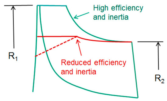
Figure 7.
Inertia reduction in a turbine wheel.
The preliminary design of the blade turbine is an essential first step in the design of a new turbomachine. A more advanced preliminary design used together with an advanced CFD method can result in a very effective turbine. ANSYS employs Vista RTD for the preliminary design, which allows development from initial ideas into full 3D geometry designs. Since the engine modelling was done in GT-Power, the engine data was imported in Vista RTD to obtain the first sketches of the blade design. An essential feature of Vista RTD is that for specific blade data input, it is possible to predict some performance factors of the turbine, such as the efficiency or the loss. The boundary conditions imported in the operating conditions in ANSYS were the output results from the engine model from GT-Power. The used operating conditions are shown in Table 2. Also, air properties are considered as fluid specifications.
Table 2.
Operating conditions used in Vista RTD.
The next step was to import the single stator blade in a feature called Turbogrid. ANSYS Meshing is an automated high-performance product. The mesh validation was implemented through many trails with different parameters to achieve accurate results. The student version of Turbogrid was employed. The total number of nodes was limited to 512,000; therefore, the option of the target number of nodes was chosen and set to be 210,000 nodes to make sure that the total number would not exceed the limitation of the nodes after adjustments.
Testing turbochargers under steady flow conditions, even though it does not faithfully reproduce real engine operating conditions, is the standard procedure followed by several manufacturers. The mesh for the rotor of the radial turbine was imported into the CFX setup. The rotor domain option was selected to be rotating, and the working fluid was air ideal gas with a pressure of one bar. Several results regarding inlet and outlet pressure and temperature were obtained from the GT-Power modelling. From the fluid model tab, the heat transfer was set to total energy and turbulence to shear stress transport. The rotor inlet had a total pressure of 195 kPa and static temperature 995 K. The outlet was defined with a static pressure of one bar. Inlet walls that were included were set as no-slip and smooth, and on the other hand, the rotor shroud frame type was rotating due to the mesh moving. The rotor blade tip named tip ggi was defined with the interface model with a general connection, which affects the loss between the shroud and wall. Lastly, before the simulation was run, from the solver control, the residual target was set to 0.0001 and the maximum iterations to 200.
Despite using a specific method for the design of the radial blade, a different approach was used to structure the blade for the axial turbine. Since the turbocharger design is a serial two-stage turbocharger, first, the results from the radial turbine were gathered; therefore, the correct conditions for the axial design could be calculated. As mentioned in Section 2, axial turbines are not commonly used in the automation industry; therefore, a different process for the design was used. With the help of a Matlab code by adapting the free vortex axial blade equations, the radial turbine boundary results were imported into the model and the preliminary angles of the axial turbine blade were found. The geometries can be found in the result section.
ANSYS Geometry was used to form sketches of the rotor and stator for the axial turbine (Figure 8 and Figure 9). As mentioned in the theory section, axial blades have airfoil shapes, and with the help of the sketch, the first designs were created.
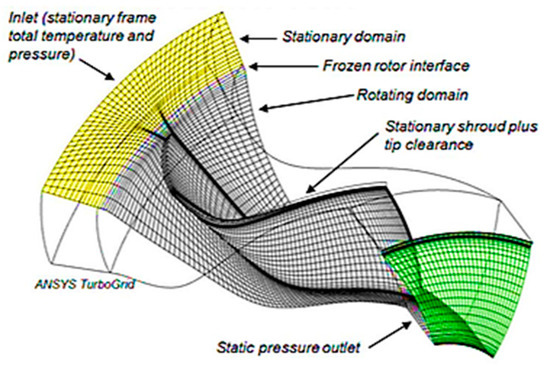
Figure 8.
Boundary conditions and mesh explained.
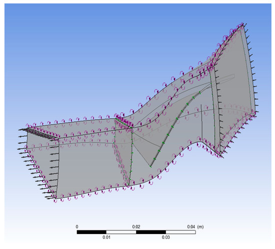
Figure 9.
Radial blade boundary setup.
With the angles of the blades gained from the Matlab code, three similar blades were created with slight differences in height for different planes, which represent the mean and tip radius and the root. Furthermore, the three parts were connected, and a 3D blade for both the rotor and stator were created. After the main part of the blade was designed, the same procedure was adopted for the radial blade, and the right flow path for the axial blade was created. Another significant factor in geometry is the ability to change several parameters onto the 3D blade that was formed.
For the meshing part, the same process was applied as the radial turbine blade (Figure 10). The boundary conditions were applied as the inlet, outlet, shroud, hub, and blade surface. On the specific blade, the target node option was used and was set to 250,000 nodes, making sure it would not exceed the mesh limit after modifications and optimisation. For the meshing, the global mesh settings were specified first, then the local mesh settings were inserted, the mesh was previewed and generated, and the mesh quality was checked.
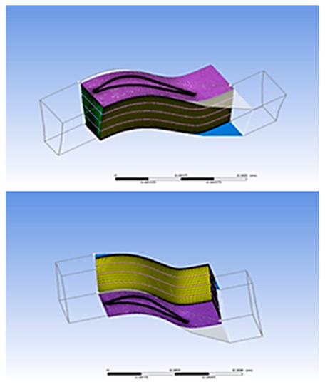
Figure 10.
Rotor blade mesh.
After meshing the stator and rotor, they were imported into CFX, where the boundary conditions were applied. The stator was selected to be stationary and the rotor was set as rotating around the z-axis. The working fluid was considered as air ideal gas at one bar, with the heat transfer set to total energy and shear stress transport for turbulence. The stator domain was stationery, with an inlet relative pressure of 200 kPa and heat transfer of 900 K. The rotor outlet was set on static pressure at 134 kPa. For the rotor shroud, the boundary type was a wall, and the frame type was chosen to be rotating as the rotor mesh has to move. Boundary details for the walls were defined as no-slip and smooth. As shown in Figure 11, the blade tips were named as tip ggi with two interfaces, which, as mentioned for the radial design, controls the losses in the blade and shroud. Lastly, the domain interface for the stator and rotor was set as a general connection, and the frame change was set on the stage (mixing-plane). To obtain accurate results, the residual target was set to 0.0001 with 200 maximum iterations in the solver control.
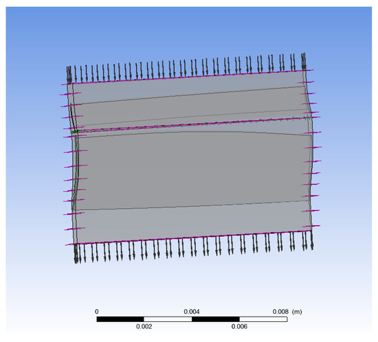
Figure 11.
Axial blade simulation setup.
As mentioned previously, regarding the blade design for the radial and axial turbines, the first sketches of the blades were based on preliminary design angles; therefore, some optimisation was needed to get excellent performance and efficiency out of the turbine. Through ANSYS, the optimisation for the radial turbine was different due to the use of bladegen and vistaRTD. There were limited optimisation capabilities, and the changes had to be done one at a time, whereas, on the other hand, the axial optimisation due to the blade being designed in Geometry directly gave the ability to optimise more than one parameters at a time.
Since the engine modelling and design of the turbines was completed, the next step was to gather the data and recalculate the two new turbine maps, the values of which were adapted in GT- Power. The first step for the development of the new map was to run the turbines at four different speeds with four different outlet pressures at a time. This process was done for both radial and axial turbines. From these simulations, it was essential to gather the mass flow rate, efficiency, pressure ratio, and the total pressure and temperature. However, to import the values in GT-Power, some calculations were done to find the reduced speed and reduced mass flow for the engine data map. The equations used were:
Furthermore, all the calculations were done, and two sets of results were obtained and ready to be imported in the turbines in GT-Power. However, the model of the engine had to be changed due to having only a single turbine connected to it. Therefore, the task was to redesign the engine in GT-Power from a single radial turbine engine to a two-stage turbine with a radial and axial turbine.
After the new engine model was completed, all the obtained values were introduced to the new turbines, and finally, the new turbines were ready and set up to run. The same case setup was used regarding the engine speeds. All the obtained results will be analysed and explained in the next section.
5. Results and Discussion
In this section of the study, a thorough analysis of the results for the designs of the two-stage radial and axial turbochargers will be presented. CFD analysis was performed on both the radial and axial turbines. Another part of this section shows and discusses the engine modelling simulation results, representing the achieved power and torque curves with the stock turbo and with the newly designed two-stage turbo system and showing whether any improvements in power or efficiency were achieved.
As mentioned above, the engine modelled in GT-Power was made to represent the engine from a MAN 6.9 L six-cylinder truck. From GT-Power, the power and torque graphs are very similar, proving that the modelled engine performs the same.
In Figure 12, the image represents the torque and power graph gained from GT-Power corresponding to the MAN engine specification. The same speeds were used to achieve these graphs.
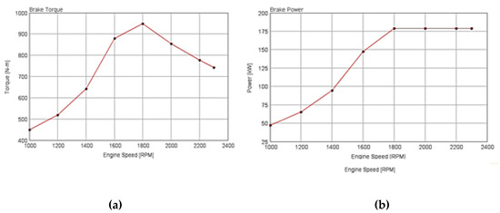
Figure 12.
(a) Engine brake torque and (b) power curves at full load.
By comparing the two power graphs from Figure 12, it is obvious that the GT-Power graph is nearly identical to the one given from the specification sheet of the MAN engine.
For the design of the blades for the two turbochargers, the engine speed chosen from GT-Power was 1800 rpm as it was the most efficient point. Figure 13 shows the efficiency and speed maps at the same rpms used to generate the torque and power curves as in Figure 12.
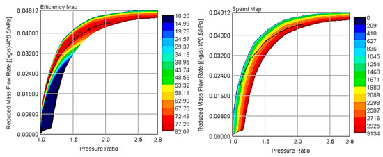
Figure 13.
Efficiency and speed map from GT-Power.
For the design and modelling of the radial turbine, some calculations were used, but the main part was done using Vista RTD in ANSYS. From the blade software, the preliminary angles were found. Table 2 shows the preliminary design parameters for the radial turbine. As the radial turbine blade geometries were given by a turbine software, it gave the ability to check the efficiencies and losses only by changing some parameters. The most efficient result was given with the following specifications:
- Blade number: 13;
- Hub radius: 15.1 mm;
- Hub exit height: 23.727 mm;
- Tip radius: 41.5 mm;
- Tip width: 13.337; and
- Axial length: 42 mm.
By using the above geometries, the radial turbine was designed as shown in Figure 14, and after running the CFD simulation, the results shown in Table 3 were achieved.
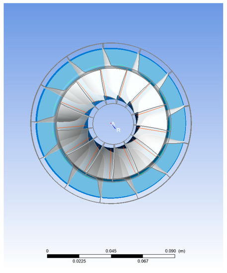
Figure 14.
Radial design.
Table 3.
Preliminary design parameters for radial blade.
Figure 15 shows the velocity streamlines. The flow direction shown by the arrows indicates that there is some turbulence occurred due to the dome design’s miss functions.
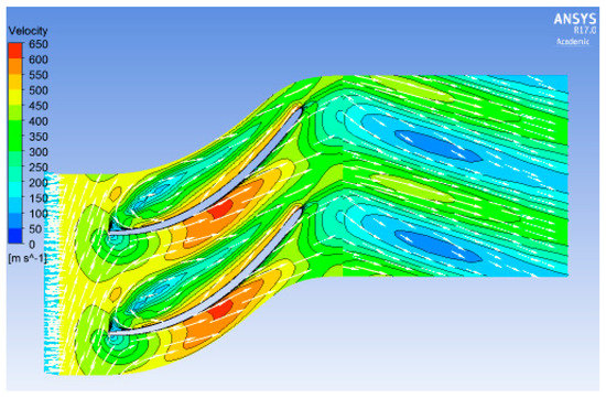
Figure 15.
Radial turbine velocity streamlines.
The red colour shows where shockwaves occurred on the blade, orange parts demonstrate the blades regions that have the possibility of a high flow, and the remaining colours illustrate the low flow regions.
The equations for the preliminary design calculations as well as some boundary conditions for the radial design were imported to a Matlab code. Table 4 includes the preliminary design geometries produced by the code to be used to design the axial turbine.
Table 4.
Preliminary design calculations.
Also, the tip radius () was calculated to be 41.5 mm and h = 0.02. By having all the values, rt and rh were found with the following equations:
The final setup that was used for the axial turbine was as follows. The rotor speed was set to 78,500 rpm, the rotor outlet pressure was 134 kPa, and the inlet temperature was set to 900 k and an inlet pressure of 200 kPa. The performance results gathered from CFX are shown in Table 5.
Table 5.
Overall performance of the turbine.
Figure 16 demonstrates the axial velocity flow. Figure 17 shows the relative Mach number, where in this case, the Mach number is less than 1.00, resulting in a subsonic turbine.
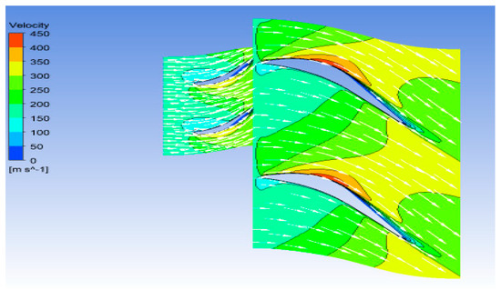
Figure 16.
Axial velocity flow.
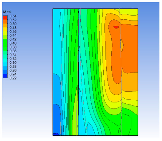
Figure 17.
Axial Mach number.
The CFD result simulations for the axial turbine with the stator and rotor are shown in Figure 18. There are several vortices generated on the blades that might be caused by the distance of the clearance between the shroud and the blade’s tip. Another reason might be the friction of the walls on the blades. Figure 19 demonstrates the final 3D design of the rotor and stator assembled together in ANSYS.
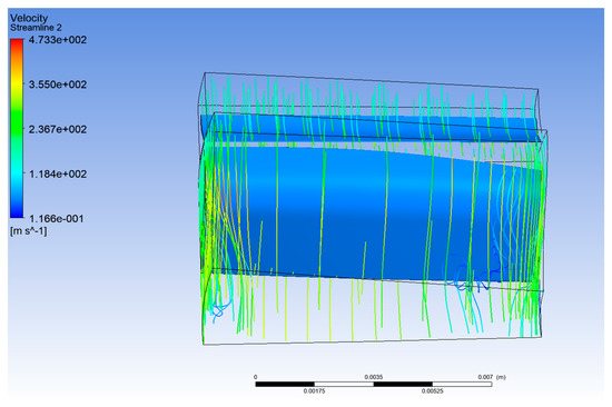
Figure 18.
Axial turbine stator and rotor velocity streamlines.
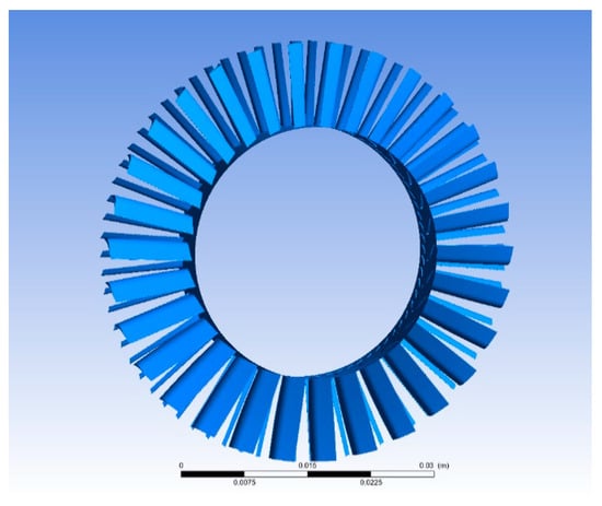
Figure 19.
Final 3D design of the rotor and stator.
Since this investigation aimed to design a two-stage radial/axial turbocharger, as mentioned previously, two sets of engines were modelled in GT-Power. The first one had a single turbo as the original engine and the second one was modified for the engine to work with the two-stage turbo system. With the new map data imported in GT-Power, the new power and torque curves are shown in Figure 20.
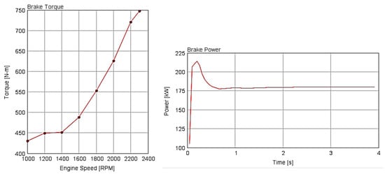
Figure 20.
New power and torque curves.
The above graphs indicate that the torque keeps increasing as the rpms increase but does not settle down, which is not a trend, whereas, on the other hand, the power curve shows an increase in power and then it stabilises as it should. After running the new modified engine with the new turbo system, a comparison of the results can be seen below in Table 6 and Table 7.
Table 6.
Initial engine data (single turbo), engine speed presents the cycle average speed; BSFC is the brake specific fuel consumption.
Table 7.
New engine data (two-stage turbo), engine speed presents the cycle average speed; BSFC is the brake specific fuel consumption.
By comparing the initial engine data with the new data, it is evident that there is a small increase in the engine’s power and torque but only at 2300 rpm. From the tables, it is visible that the points that had to decrease have increased, and the engine is lacking power in comparison with the initial model. Further, the rest of the data does not seem to be working normally as was expected. The new efficiency and power maps are shown in Figure 21.
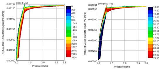
Figure 21.
New efficiency and speed map.
6. Conclusions
The specific investigation was about the design of a two-stage turbo system, which contained a radial and an axial turbine connected in series. From this design, the goal was to achieve better performance and torque while maintaining efficiency and reducing the rotating inertia of the rotor. This new concept is only implemented by Honeywell with the cooperation of Volvo trucks and has managed to gain fuel efficiency. This research is an attempt to create a novel method to confirm the benefit of the newly adopted concept. Moreover, two engines were simulated in GT-Power, one with a single radial turbine and the other with a two-stage radial/axial turbo system. The results for the radial and axial turbines indicated an efficiency of 83.4% and 81.74%, respectively.
Nevertheless, the two-stage system, as shown in the results section, did not operate as expected. Therefore, a sum of alternations needs to be incorporated into the system to improve the accuracy of the final engine model with the two-stage turbo system. The presented results in this study can be considered as a foundation for further improvement.
Further work that could be applied to this study is creating better and in-depth optimisation to achieve higher efficiencies with power at the same time. By having an efficient turbine that produces enough power, the new data can be imported in the GT-Power maps and the simulations can be rerun to check the differences in power, torque, and fuel efficiency. Lastly, a complete drive cycle of the new engine model with the two-stage turbo system can be done in GT-Power to obtain the actual working conditions on how the engine would perform in reality.
Author Contributions
C.P. was the research student that conducted the detailed study and wrote the paper assisted by S.S.S. who also edited the paper. A.P. conceived of the project, created the layout of the investigations, and checked the computational outcome of the resultant modelling effort and subsequent discussion.
Funding
This research received no external funding.
Conflicts of Interest
The authors declare no conflict of interest.
References
- Bauer, K.H.; Balis, C.; Donkin, G.; Davies, P. The Next Generation of Gasoline Turbo Technology. 2012. Available online: http://turbo.honeywell.com/assets/pdfs/120202-EN-Vienna-Motor-Symposium-Presentation.pdf (accessed on 8 June 2017).
- Anon, N.D. Vehicle Tax Rates. Available online: https://www.gov.uk/vehicle-tax-rate-tables (accessed on 10 June 2017).
- More, S. Dual Boost Turbocharger. Int. J. Mech. Prod. Eng. 2016, 4, 1–7. [Google Scholar]
- Feneley, A.J.; Pesiridis, A.; Andwari, A.M. Variable Geometry Turbocharger Technologies for Exhaust Energy Recovery and Boosting—A Review; Elesevir Ltd.: London, UK, 2016. [Google Scholar]
- Cadle, R.; Giebert, D.; Mohamed, A.; Pees, S.; Oakes, M. Ultra high efficiency two-stage turbocharging system. In Proceedings of the 12th International Conference on Turbochargers and Turbocharging, Institution of Mechanical Engineers, London, UK, 17–18 May 2016. [Google Scholar]
- Honeywell. Available online: https://turbo.honeywell.com/our-technologies/twostage-serial-turbo/ (accessed on 30 August 2017).
- Cadle, R.; Giedbert, D.; Mohamed, A.; Pees, S.; Oakes, M. Ultra High Efficiency Two Stge Turbocharging System; Honeywell: Torrance, CA, USA, 2012. [Google Scholar]
- Bernhardt Luddecke, D.F.J.E. Mixed Flow Turbines for Automotive Turbocharger Applications; Hindawi: Heidberg, Germany, 2011. [Google Scholar]
- Nice, K. How Turbochargers Work, How Stuff Works. Available online: http://auto.howstuffworks.com/turbo.htm (accessed on 30 August 2017).
- Rahnke, C.J. Axial Flow Automotive Turbocharger; ASME: Hayward Ann Arbor, MI, USA, 1985. [Google Scholar]
- Barrans, S.; Allport, J.; Khodabakhshi, G. Turbocharger Structural Integrity. Manuf. Ind. Eng. 2014, 13, 1–5. [Google Scholar] [CrossRef][Green Version]
- Rakopoulos, C.D.; Giakoumis, E.G. Diesel Engine Transient Operation; Springer: Athens, Greece, 2009. [Google Scholar]
- Wright, G. Diesel Class. Available online: http://dieselclass.com/Engine%20Files/VGT%20Turbochargers%209-05.pdf (accessed on 12 June 2017).
- Baskharone, E.A. Principles of Turbomachinery in Air Breathing Engines; Cambridge University Press: Cambridge, MA, USA, 2006. [Google Scholar]
- Khader, M. Optimised Radial Turbine Designl; City University: London, UK, 2014. [Google Scholar]
- Ventura, C.A.; Jacobs, P.A.; Rowlands, A.S.; Petrie-Repar, P.; Sauret, E. Preliminary Design and Performance Estimation of Radial Inflow Turbines: An Automated Approach. Fluids Eng. 2012, 134, 031102. [Google Scholar] [CrossRef]
- Huntsman, I.; Hodson, H.P.; Hill, S.H. The Design and Testing of a Radial Flow Turbine for Aerodynamic Research; ASME: New York, NY, USA, 1991. [Google Scholar]
- Zungia, Y.S.P. Design of an Axial Turbine and Thermodynamic Analysis and Testing of a ko3 Turbocharger; Massachusetts Institute of Technology: Cambridge, MA, USA, 2011. [Google Scholar]
- Pesiridis, A. Issues in the integration of active control turbochargers with internal combustion engines. Int. J. Automot. Technol. 2012, 13, 873–884. [Google Scholar] [CrossRef]
- Pesiridis, A. The application of active control for turbocharger turbines. Int. J. Eng. Res. 2012, 13, 385–398. [Google Scholar] [CrossRef]
- Cox, G. Challenges in the Design of Radial Turbines for Small Gasoline Engines; PCA Engineers Limited: Lincoln, UK, 2014. [Google Scholar]
© 2019 by the authors. Licensee MDPI, Basel, Switzerland. This article is an open access article distributed under the terms and conditions of the Creative Commons Attribution (CC BY) license (http://creativecommons.org/licenses/by/4.0/).