DFT-Based Identification of Oscillation Modes from PMU Data Using an Exponential Window Function

Abstract

The characteristics of oscillation modes, such as interarea, regional, and subsynchronous modes, can vary during a power system fault, which can cause switching and control actions in the power system. Transient data of the modal response due to such a fault can be acquired through phasor measurement units (PMUs). When the transient data have a long duration, it is desirable to perform modal identification separately on each segment of the transient data, so as to reflect the varying characteristics of oscillation modes. A conventional discrete Fourier transform (DFT)-based method for parametric modal identification cannot be efficiently applied to such a segment dataset. In this paper, a DFT-based method with an exponential window function is proposed to identify oscillation modes from each segment of transient data in PMUs. This window function allows the application of the least squares method (LSM) for modal identification in the same manner as the conventional method. The accuracy of identification of the proposed method is compared with those of the conventional method and a Prony method through synthetic data of transient responses. Its feasibility is also verified by identifying real-world oscillation modes from transient data in PMUs.

1. Introduction

Power systems can have various oscillation modes, such as interarea, regional, and subsynchronous modes. An interarea mode has an oscillation frequency of less than 1 Hz and oscillates in opposite directions between faraway regions in the power system [1]. A regional mode has an oscillation frequency between 1 and 2 Hz and oscillates among generators in a region of the power system. A subsynchronous mode has an oscillation frequency above 5 Hz and oscillates because of interactions among the mechanical turbine generator system, the electrical power transmission system of series compensation, and electronic devices in high-voltage DC (HVDC) transmission systems and flexible AC transmission systems (FACTS) [2,3]. These oscillations can have a severe effect on the stability and transfer capacity of the power system. It is essential to monitor and control the oscillation modes for efficient operation of the power system.

Waveforms of modal oscillations can be observed well in a transient response of power systems owing to a sudden disturbance caused by a fault in the power system or a large change in the power load [4,5,6]. The Fourier transform magnitude of this transient response has a distinguishable peak at the oscillation frequency of each mode, owing to low modal damping. Nowadays, the modal oscillation frequencies and damping factors can be estimated from the transient data, which can be obtained from measurements of the active power, phasor angle, and frequency in phasor measurement units (PMUs). Most PMUs have data measurement rates below 60 per second. Such PMU data are not suitable for identifying a subsynchronous oscillation mode with an oscillation frequency of up to 60 Hz. Some PMUs have data measurement rates above 60 per second: their data enable subsynchronous modes with low-frequency oscillations to be identified effectively [7]. Currently, PMUs are installed on transmission grids. Their installation is now expanding to distributed grids and microgrids for monitoring and protection [8,9]. PMU data on distribution grids and microgrids generally have signal-to-noise ratios (SNRs) lower than transmission grids.

Parametric identification of oscillation modes can be performed on transient data in the time domain or frequency domain. A variety of time-domain-based methods, such as Prony [10], Matrix pencil [11], and Hankel total least squares (HTLS) methods, have been reported so far [12]. They fit transient data to their autoregressive (AR) models of oscillation modes directly. These methods are very sensitive to noise, which inevitably means that many fake modes of noise are added to the AR model. The fake mode number can be assigned through singular value decomposition (SVD) [10], which requires a little computation time. A discrete Fourier transform (DFT)-based method of parametric modal identification was designed to curve-fit DFT coefficients of transient data into a transfer function of oscillation modes in the frequency domain [13,14]. Such curve-fitting is performed on small frequency ranges around each modal peak in the DFT magnitude, which can lead to a short computation time compared to that involved in the time-domain methods. However, this method can be applied for identification of stable modes whose oscillations converge to zeros in the transient data.

Oscillation phenomena in power systems can sometimes last for a long duration. In such transient data, oscillation modes can be unstable or typically exhibit non-stationary behaviors due to the nature of switching events and other control actions in the power system [15,16]. This means that the oscillation frequency and damping factors may vary slightly from time to time in transient data. For this reason, it is necessary to split such transient data into many segments and identify oscillation modes from each segment sequentially. A smaller segment is more desirable as transient data are less stationary. A conventional DFT-based method cannot be applied directly to the segment where modal oscillations do not converge to zero. For the application of the conventional DFT-based method, a window function is required to force the modal oscillations to converge to zero in the segment.

In this paper, a DFT-based method with an exponential window function is proposed to identify oscillation modes from each segment of transient data in PMUs. This exponential function enables the conventional DFT-based method to be applied to each segment of transient data. The identification accuracy of the proposed methods is compared with conventional DFT-based and Prony methods through modal identification using synthetic data of transient responses. Its feasibility is demonstrated by identifying oscillation modes from PMU transient data of power systems in the United States and Central America.

2. Conventional Modal Identification in Power Systems

2.1. Models for Modal Identification in Time and Frequency Domains

An oscillation mode in the power system is triggered by a sudden disturbance caused by a power event such as a line fault, generator trip, or huge load change. This disturbance can be modeled as an impulse function at the beginning of the power event. A modal oscillation owing to the disturbance can be expressed as a second order differential equation. When there are $K$ oscillation modes in the power system, their transient response after the event can be given as the following sum $y\left(t\right)$ of sinusoidal functions with the magnitudes of exponential functions:

$$y\left(t\right)={\sum }_{k=1}^K{q}_k\left(t\right),q_k\left(t\right)=A_k{e}^{-{\xi }_{k}t} \sin \left({\omega }_{k}t+{\theta }_k\right),0\le t\le t_e$$

(1)

where $q_k\left(t\right)$ is the k-th mode with a damping factor of ${\xi }_k$ and an oscillation frequency of ${\omega }_k=2\pi f_k$, $f_1<f_2\cdots <f_K$. Here, $A_k$ and ${\theta }_k$ are the amplitude and phase angle of the k-th mode, respectively. The natural frequency and damping ratio of the k-th mode can be calculated to be ${\varpi }_k={\omega }_k\sqrt{1-{\mathsf{\zeta }}_k^2}$ and ${\mathsf{\zeta }}_k={\xi }_k/{\varpi }_k$, respectively. The initial time of a power event is denoted as $t$ = 0 and $t_e$ is the duration of the transient response. The modal parameters ${\xi }_k$, $f_k$, $A_k$, and ${\theta }_k$ can vary slightly from time to time, according to control actions of the power system after the event.

The Laplace transform of $y\left(t\right)$ is given as the following for $Y\left(s\right)$:

$$Y\left(s\right)={\int }_0^{t_e}y\left(t\right)e^{-st}dt={\sum }_{k=1}^K\left(Q_k\left(s\right)-E_k\left(s\right)\right)$$

(2)

$$Q_k\left(s\right)=A_k\frac{\left(s+{\xi }_k\right)\sin {\theta }_k+{\omega }_k\cos {\theta }_k}{s^2+2{\xi }_{k}s+{\xi }_k^2+{\omega }_k^2},E_k\left(s\right)=A_k\frac{\left(s+{\xi }_k\right)\sin \left({\omega }_k{t}_e+{\theta }_k\right)+{\omega }_k\cos \left({\omega }_k{t}_e+{\theta }_k\right)}{s^2+2{\xi }_{k}s+{\xi }_k^2+{\omega }_k^2}{e}^{-\left(s+{\xi }_k\right)t_e}$$

(3)

where $E_k\left(s\right)$ has a transcendental function of $e^{-\left(s+{\xi }_k\right)t_e}$. Here, $Y\left(s\right)$ becomes a rational function if $E_k\left(s\right)$ is ignorable, which is satisfied under the conditions of stable oscillation modes with $e^{-{\xi }_k{t}_e}\approx 0$, $t_e>t$. The Fourier transform of $y\left(t\right)$ is obtained as $Y\left(j\omega \right)$, where $j=\sqrt{-1}$. The modal parameters ${\xi }_k$, $f_k$, $A_k$, and ${\theta }_k$ can be estimated in the frequency domain by curve-fitting $Y\left(j\omega \right)$ into DFT coefficients of transient data in PMUs.

For modal identification in the time domain, the continuous-time signal $y\left(t\right)$ should be converted into a discrete-time signal, which is represented with an autoregressive (AR) model. The impulse invariance transform [17] is applied to this conversion with a sampling interval of $T_s$. Then, the AR model is given as

$$y\left[n\right]={\sum }_{k=1}^K{q}_k\left[n\right],q_k\left[n\right]=-d_{k,1}{q}_k\left[n-1\right]-d_{k,2}{q}_k\left[n-2\right]0\le n<N$$

(4)

$$d_{k,1}=-2e^{-{\xi }_k{T}_s}\cos \left({\omega }_k{T}_s\right),d_{k,2}=e^{-2{\xi }_k{T}_s}$$

where $y\left[n\right]=\mathrm{y}\left(n{T}_s\right)$ and $N$ is the data number for $t_e=N{T}_s$. The Prony method can estimate the modal parameters ${\xi }_k$, $f_k$, $A_k$, and ${\theta }_k$ by fitting the AR model into transient data in PMUs.

Actually, PMU data contain measurement noise [18] and a DC component [19,20]. The measurement noise can generally be assumed to be white noise. The DC component is an instantaneous drop or rise that reflects any imbalances between the supply and demand of active power in the power system. The DC component as well as the measurement noise degrades the identification accuracy of the time-domain-based method more severely than that of the frequency-domain-based method. In this paper, a second-order Butterworth digital bandpass filter is introduced for pre-processing to reject the DC component from transient data in PMUs. Its lower cutoff frequency is designed to be 0.01 Hz, which is far away from the lowest frequency of interarea oscillations. Its upper cutoff frequency is set at ($f_s/2-0.01)$ Hz, where $f_s=1/T_s$. This bandwidth leads to ignoring the filtering effects on $y\left[n\right]$ and the measurement noise. Then, a pre-filtered signal from transient data in PMUs can be given as the following for $y_w\left[n\right]$:

$$y_w\left[n\right]=y\left[n\right]+w\left[n\right],0\le n<N$$

(5)

where $w\left[n\right]$ is the measurement noise.

The magnitude of $Y\left(j\omega \right)$ has sharp peaks around ${\omega }_k$ due to low modal damping. This indicates that the modal number $K$ can be determined by counting the number of dominant peaks in the DFT magnitude of $y_w\left[n\right]$. The shape of these peaks can be more apparent as the DFT frequency resolution is smaller; the resolution is defined as the frequency interval between two adjacent DFT coefficients. For this reason, zero data values are padded properly to $y_w\left[n\right]$. Then, the DFT coefficient of $y_w\left[n\right]$ was calculated as the following for $Y_w\left[m\right]$:

$$Y_w\left[m\right]=\frac{2}{N}{\sum }_{k=0}^{N-1}{y}_w\left[k\right]e^{-\frac{j2\pi mk}{M}},0\le m<M$$

(6)

where $M$ is the total data number, including the zero-padding data, and the index $m$ corresponds to $m/\left(M{T}_s\right)$ Hz in the frequency domain. Frequencies at the peaks are measured as ${\tilde{f}}_k$, $k=1,2,\cdots ,K,$ and are rearranged as (${\tilde{f}}_1<{\tilde{f}}_2<\cdots <{\tilde{f}}_K$) according to their size. They can be used effectively for the discrimination of fake modes in the time-domain-based method and for assignment of curve-fitting frequency ranges per oscillation mode in the frequency-domain-based method.

2.2. Conventional DFT-Based Method

A conventional DFT-based method can be applied to $Y\left(j\omega \right)$ only if $Y\left(s\right)$ is a rational function, which is satisfied under the condition of $E_k\left(s\right)\approx 0$ in Equation (3). In this condition, $Y\left(s\right)$ can be represented with $4K$ coefficients of $a_k$ and $b_k$, $k=1,2,\cdots ,2K$ as

$$Y\left(s\right)={\sum }_{k=1}^K{Q}_k\left(s\right)=\frac{b_1{s}^{2K-1}+ \cdots +b_{2K-1}s+b_{2K}}{s^{2K}+a_1{s}^{2K-1}+ \cdots +a_{2K-1}s+a_{2K}}$$

(7)

Each $Q_k\left(s\right)$ is obtained from $a_k$ and $b_k$ by factorizing $Y\left(s\right)$ through its characteristic root ${\alpha }_k$ of the k-th oscillation mode as

$$Q_k\left(s\right)=\frac{{\beta }_k}{s-{\alpha }_k}+\frac{{\beta }_k^{*}}{s-{\alpha }_k^{*}}$$

(8)

where ${\beta }_k$ is a complex number corresponding to ${\alpha }_k$ and * represents the conjugate of a complex number. The k-th modal parameters of ${\omega }_k=2\pi f_k$, ${\xi }_k$, $A_k$, and ${\theta }_k$ in Equation (1) can be calculated from ${\alpha }_k$ and ${\beta }_k$ as follows:

$${\omega }_k=\left|\mathrm{Im}\left\{{\alpha }_k\right\}\right|,{\xi }_k=-\mathrm{Re}\left\{{\alpha }_k\right\},A_k=2\left|{\beta }_k\right|,{\theta }_k=\angle \left(\mathrm{Im}\left\{{\beta }_k^{*}\right\}+j\mathrm{Re}\left\{{\beta }_k\right\}\right)$$

(9)

where $|·|$ and $\angle (·)$ represent the magnitude and angle of a complex number, respectively.

The K oscillation modes in $Y\left(s\right)$ of Equation (7) are identified through estimation of the coefficients $a_k$ and $b_k$, which is accomplished by curve-fitting $Y_w\left[m\right]$ of Equation (6) into $Y\left(j\omega \right)$ of Equation (7) in the frequency domain. To apply the LSM for estimation of $a_k$ and $b_k$, the complex values of Equation (7) by $s=j\omega$ can be divided into the two following linear equations for $a_k$ and $b_k$ in the real and imaginary parts:

$${\left(-1\right)}^{K-1}{\omega }^{2K-2}{a}_2+\cdots +\left(-1\right)a_{2K}+\mathrm{Re}\left\{\frac{{\left(j\omega \right)}^{2K-1}}{Y\left(j\omega \right)}\right\}{b}_1+\cdots +\mathrm{Re}\left\{\frac{\left(j\omega \right)}{Y\left(j\omega \right)}\right\}{b}_{2K-1}+\mathrm{Re}\left\{\frac{1}{Y\left(j\omega \right)}\right\}{b}_{2K}={\left(-{\omega }^2\right)}^K$$

(10)

$${\left(-1\right)}^K{\omega }^{2K-1}{a}_1+\cdots +\left(-1\right)\omega a_{2K-1}+\mathrm{Im}\left\{\frac{{\left(j\omega \right)}^{2K-1}}{Y\left(j\omega \right)}\right\}{b}_1+\cdots +\mathrm{Im}\left\{\frac{\left(j\omega \right)}{Y\left(j\omega \right)}\right\}{b}_{2K-1}+\mathrm{Im}\left\{\frac{1}{Y\left(j\omega \right)}\right\}{b}_{2K}=0$$

(11)

where $\mathrm{Re}\{·\}$ and $\mathrm{Im}\{·\}$ represent the real and imaginary parts of a complex number, respectively.

To reduce the noise effect as well as the computation burden for modal identification, it is desirable to perform curve-fitting on $Y_w\left[m\right]$ around ${\tilde{f}}_k$, where most of the modal oscillation power is concentrated. Thus, $Y_w\left[m\right]$ of the following frequency ranges can be applied for the curve-fitting:

$$\left|{\tilde{f}}_k-f\right|\le f_c, k=1,2,\cdots ,K$$

(12)

where $f_c$ is a design parameter. Oscillation frequencies of interarea and regional modes can be distributed at an interval of up to 0.1 Hz in the frequency domain. Subsynchronus frequencies can be typically distributed farther than 1 Hz from each other. For these reasons, the curve-fitting frequency range for interarea modes and regional modes is set to $f_c=0.05$ Hz, and that for synchronous modes is set to $f_c=0.5$ Hz in this paper.

Because a mode has four unknown parameters, namely ${\omega }_k$, ${\xi }_k$, $A_k$, and ${\theta }_k$, the sample number $M_c$ of the angular frequency $\omega$ in Equations (10) and (11) per mode should be greater than 2. The number $M_c$ was chosen experimentally to be 5 by comparing the identification accuracy obtained during the simulations discussed in Section 3.2. Then, $M$ is calculated from $M_c=2M{f}_c{T}_s+1$. When angular frequency samples per mode in Equation (12) are given as ${\omega }_{k,l}$, $0\le l<M_{\mathit{C}}$, the curve-fitting of $Y\left(j\omega \right)$ of Equations (10) and (11) represents the following matrix form [13]:

$$\mathit{B}\mathit{R}=\mathit{D},\mathit{B}=[{\mathit{B}}_1{\mathit{B}}_2]$$

(13)

$$\mathit{R}={[a_1 a_2\cdots a_{2K-1} a_{2K} b_1 b_2\cdots b_{2K-1} b_{2K}]}^T,\mathit{D}={[{\left(-{\omega }_{1,1}^2\right)}^K 0 {\left(-{\omega }_{1,2}^2\right)}^K 0\cdots {\left(-{\omega }_{K,M}^2\right)}^K 0]}^T$$

(14)

$${\mathit{B}}_1=\left[\begin{array}{ccccc}0& {\left(-1\right)}^{K-1}{\omega }_{1,1}^{2K-2}& \cdots & 0& -1\\ {\left(-1\right)}^K{\omega }_{1,1}^{2K-1}& 0& \cdots & -{\omega }_{1,1}^2& 0\\ 0& {\left(-1\right)}^{K-1}{\omega }_{1,2}^{2K-2}& \cdots & 0& -1\\ {\left(-1\right)}^K{\omega }_{1,2}^{2K-1}& 0& \cdots & {\omega }_{1,2}^2& 0\\ ⋮& ⋮& ⋮& ⋮& ⋮\\ 0& {\left(-1\right)}^{K-1}{\omega }_{K,M}^{2K-2}& \cdots & 0& -1\\ {\left(-1\right)}^K{\omega }_{K,M}^{2K-1}& 0& \cdots & -{\omega }_{K,M}^2& 0\end{array}\right]$$

(15)

$${\mathit{B}}_2=\left[\begin{array}{cccc}\mathrm{Re}\{\frac{{\left(j{\omega }_{1,1}\right)}^{2K-1}}{Y\left(j{\omega }_{1,1}\right)}\}& \mathrm{Re}\{\frac{{\left(j{\omega }_{1,1}\right)}^{2K-2}}{Y\left(j{\omega }_{1,1}\right)}\}& \cdots & \mathrm{Re}\{\frac{1}{Y\left(j{\omega }_{1,1}\right)}\}\\ \mathrm{Im}\{\frac{{\left(j{\omega }_{1,1}\right)}^{2K-1}}{Y\left(j{\omega }_{1,1}\right)}\}& \mathrm{Im}\{\frac{{\left(j{\omega }_{1,1}\right)}^{2K-2}}{Y\left(j{\omega }_{1,1}\right)}\}& \cdots & \mathrm{Im}\{\frac{1}{Y\left(j{\omega }_{1,1}\right)}\}\\ \mathrm{e}\{\frac{{\left(j{\omega }_{1,2}\right)}^{2K-1}}{Y\left(j{\omega }_{1,2}\right)}\}& \mathrm{Re}\{\frac{{\left(j{\omega }_{1,2}\right)}^{2K-2}}{Y\left(j{\omega }_{1,2}\right)}\}& \cdots & \mathrm{Re}\{\frac{1}{Y\left(j{\omega }_{1,2}\right)}\}\\ \mathrm{Im}\{\frac{{\left(j{\omega }_{1,2}\right)}^{2K-1}}{Y\left(j{\omega }_{1,2}\right)}\}& \mathrm{Im}\{\frac{{\left(j{\omega }_{1,2}\right)}^{2K-2}}{Y\left(j{\omega }_{1,2}\right)}\}& \cdots & \mathrm{Im}\{\frac{1}{Y\left(j{\omega }_{1,2}\right)}\}\\ ⋮& ⋮& ⋮& ⋮\\ \mathrm{Re}\{\frac{{\left(j{\omega }_{K,M}\right)}^{2K-1}}{Y\left(j{\omega }_{K,M}\right)}\}& \mathrm{Re}\{\frac{{\left(j{\omega }_{K,M}\right)}^{2K-2}}{Y\left(j{\omega }_{K,M}\right)}\}& \cdots & \mathrm{Re}\{\frac{1}{Y\left(j{\omega }_{K,M}\right)}\}\\ \mathrm{Im}\{\frac{{\left(j{\omega }_{K,M}\right)}^{2K-1}}{Y\left(j{\omega }_{K,M}\right)}\}& \mathrm{Im}\{\frac{{\left(j{\omega }_{K,M}\right)}^{2K-2}}{Y\left(j{\omega }_{K,M}\right)}\}& \cdots & \mathrm{Im}\{\frac{1}{Y\left(j{\omega }_{K,M}\right)}\}\end{array}\right]$$

(16)

The LSM is applied to Equation (13) by replacing $Y\left(j{\omega }_{k,l}\right)$ in $\mathit{B}$ with $Y_w\left[m\right]$ in Equation (6), where the index $m$ corresponds to ${\omega }_{k,l}$ in the frequency domain. Estimates of $a_k$ and $b_k$ are obtained as $\mathit{R}={({\mathit{B}}^T\mathit{B})}^{-1}{\mathit{B}}^T\mathit{D}$. Here, α_k and β_k in Equation (8) are obtained from the estimated $a_k$ and $b_k$. The k-th modal parameters are estimated from ${\alpha }_k$ and ${\beta }_k$ as ${\widehat{f}}_k$, ${\widehat{\xi }}_k$, ${\widehat{A}}_k$, and ${\widehat{\theta }}_k$ through Equation (9).

2.3. Prony Method with SVD

In a time-domain-based method, $y_w\left[n\right]$ in Equation (4) is expressed with the coefficient number of $2K$ for an AR model of oscillation modes. A Prony method estimates the AR model coefficients using the LSM, whose estimation error is extremely dependent on the noise $w\left[n\right]$ in $y_w\left[n\right]$. The estimation error can be reduced significantly by adding fake modes of the noise to the AR model. When the number of characteristic roots in $y_w\left[n\right]$ is assigned to $P\gg 2K$, including fake modes, $y_w\left[n\right]$ can be represented with unknown coefficients $c_p$, $p=1, 2,\cdots ,P$, employing the following AR model:

$$y_w\left[n\right]=-{\sum }_{p=1}^P{c}_p{y}_w\left[n-p\right],P\le n<N$$

(17)

In this paper, $P$ is set to the largest integer smaller than $N/3$ [21].

The coefficients $c_p$ are obtained from the following matrix equation [10,13]:

$$\mathit{H}\mathit{C}=\mathit{G},\mathit{H}=-\left[\begin{array}{c}{y}_w\left[P-1\right]\\ y_w\left[P\right]\\ ⋮\\ y_w\left[N-2\right]\end{array}\begin{array}{c}{y}_w\left[P-2\right]\\ y_w\left[P-1\right]\\ ⋮\\ y_w\left[N-3\right]\end{array}\begin{array}{c}\cdots \\ \cdots \\ ⋮\\ \cdots \end{array}\begin{array}{c}{y}_w\left[0\right]\\ y_w\left[1\right]\\ ⋮\\ y_w\left[N-P-1\right]\end{array}\right],\mathit{C}=\left[\begin{array}{c}{c}_1\\ c_2\\ ⋮\\ c_P\end{array}\right],\mathit{G}=\left[\begin{array}{c}{y}_w\left[P\right]\\ y_w\left[P+1\right]\\ ⋮\\ y_w\left[N-1\right]\end{array}\right]$$

(18)

To reduce the noise effect in modal identification, SVD can be performed on the Hankel matrix $\mathit{H}$, whose singular values (SVs) can be partitioned into the following form:

$$\mathit{H}=\left[\begin{array}{cc}{\mathit{U}}_1& {\mathit{U}}_2\end{array}\right]\left[\begin{array}{cc}{\mathit{S}}_1& 0\\ 0& {\mathit{S}}_2\end{array}\right]\left[\begin{array}{c}{\mathit{V}}_1^T\\ {\mathit{V}}_2^T\end{array}\right],\frac{{\sigma }_1^2+{\sigma }_2^2+\cdots +{\sigma }_{\overline{P}}^2}{{\sigma }_1^2+{\sigma }_2^2+\cdots +{\sigma }_P^2}\ge \rho$$

(19)

where $\left[\begin{array}{cc}{\mathit{U}}_1& {\mathit{U}}_2\end{array}\right]$ and $\left[\begin{array}{cc}{\mathit{V}}_1& {\mathit{V}}_2\end{array}\right]$ are the left and the right singular vectors, respectively. Here, ${\mathit{S}}_1$ and ${\mathit{S}}_2$ are the diagonal matrices with SVs, ${\sigma }_1\ge {\sigma }_2\cdots \ge {\sigma }_P$; $\rho$ is a design parameter that functions as the rank threshold for choice of $\overline{P}$, based on which the matrix dimensions of ${\mathit{U}}_1$, ${\mathit{V}}_1$, and ${\mathit{S}}_1$ are given as $2P\times \overline{P}$, $P\times \overline{P}$, and $\overline{P}\times \overline{P}$, respectively [22]. In this paper, $\rho$ is assigned to 0.99 [10]. By truncating ${\mathit{S}}_2$ of the smallest SVs, the coefficients $c_p$ are estimated by applying the LSM to ${\mathit{U}}_1{\mathrm{S}}_1{\mathit{V}}_1^T\mathit{C}=\mathit{G}$.

Characteristic roots of the AR model of Equation (17) are obtained from estimates of $c_p$. Their oscillation frequencies and damping factors can be calculated as ${\overline{\omega }}_p=2\pi {\overline{f}}_p$ and ${\overline{\xi }}_p$, respectively:

$${\overline{\omega }}_p=\left|\mathrm{im}\left\{\ln \left({\lambda }_p\right)\right\}\right|/T_s,{\overline{\xi }}_p=-\mathrm{Re} \left\{\ln \left({\lambda }_p\right)\right\}/T_s,1\le p<P$$

(20)

where ${\lambda }_p$ is the characteristic root.

The k-th modal characteristic root ${\gamma }_k$ can be chosen to be ${\lambda }_p$, which minimizes $\left|{\tilde{f}}_k-{\overline{f}}_p\right|, p=1,2,\cdots ,P$. The k-th modal oscillation frequency and damping factor are estimated with the chosen $p$ as ${\widehat{f}}_k={\overline{f}}_p$ and ${\widehat{\xi }}_k={\overline{\xi }}_p$, respectively. Here, $y_w\left[n\right]$ can be represented with complex magnitudes ${\mu }_k$ and ${\mu }_k^{*}$ of the k-th mode, corresponding to ${\gamma }_k$ and ${\gamma }_k^{*}$ as

$$y_w\left[n\right]={\sum }_{k=1}^K({\mu }_k{\gamma }_k^n+{\mu }_k^{*}{\gamma }_k^{*n}),0\le n<N$$

(21)

The magnitude ${\mu }_k$ is calculated by applying the LSM to the above equation. Estimates of $A_k$ and ${\theta }_k$ in Equation (1) can be obtained as

$${\widehat{A}}_k=2\left|{\mu }_k\right|,{\widehat{\theta }}_k=\angle {\mu }_k+\pi /2,k=1,2,\cdots ,K$$

(22)

3. Modal Identification Methods with Exponential Window Function

3.1. Exponential Window Function for Modal Identification

A transient response of oscillation modes with a long duration can be nonstationary, owing to time-dependent control and nonlinear dynamics in the power system. To make the modal identification reflect a nonstationary phenomenon, the identification needs to be performed separately for sequential segments of the transient data. Unfortunately, the conventional DFT-based method has difficulty identifying the modes in segments where modal oscillations do not reach zero exponentially. This difficulty originates from Laplace transform of such a segment, which contains the transcendental function $E_k\left(s\right)\ne 0$ in Equation (3).

To overcome the limited use of the conventional DFT-based method, the proposed method introduces a window function into the Laplace transform. When a portion of $y\left(t\right)$ is given as $x\left(\tau \right)$, $0\le \tau <T_h$ for modal identification, the following exponential window function $h\left(\tau \right)$ is introduced to the Laplace transform of $x\left(\tau \right)$:

$$h\left(\tau \right)=e^{-{\xi }_0\tau },0\le \tau <T_h$$

(23)

where ${\xi }_0>0$ is a design parameter. The Laplace transform of $\overline{x}\left(\tau \right)=h\left(\tau \right)x\left(\tau \right)$ is given as the following $\overline{X}\left(s\right)$:

$$\overline{X}\left(s\right)={\int }_0^{T_h}\overline{x}\left(\tau \right)e^{-s\tau }d\tau ={\sum }_{k=1}^K\left({\overline{Q}}_k\left(s\right)-{\overline{E}}_k\left(s\right)\right)$$

(24)

$${\overline{Q}}_k\left(s\right)=A_k\frac{\left(s+{\xi }_k+{\xi }_0\right)\sin {\theta }_k+{\omega }_k\cos {\theta }_k}{s^2+2\left({\xi }_k+{\xi }_0\right)s+{({\xi }_k+{\xi }_0)}^2+{\omega }_k^2}$$

(25)

$${\overline{E}}_k\left(s\right)=A_k\frac{\left(s+{\xi }_k+{\xi }_0\right)\sin \left({\omega }_k{T}_h+{\theta }_k\right)+{\omega }_k\cos \left({\omega }_k{T}_h+{\theta }_k\right)}{s^2+2\left({\xi }_k+{\xi }_0\right)s+{({\xi }_k+{\xi }_0)}^2+{\omega }_k^2}{e}^{-\left(s+{\xi }_k\right)T_h}{e}^{-{\xi }_o{T}_h}$$

(26)

When $h\left(T_h\right)=e^{-{\xi }_o{T}_h}\approx 0$, ${\overline{E}}_k\left(s\right)$ is negligible, which makes $\overline{X}\left(s\right)$ approximate to a rational function with coefficients ${\overline{a}}_k$ and ${\overline{b}}_k$, as follows:

$$\overline{X}\left(s\right)=\frac{{\overline{b}}_1{s}^{2K-1}+ \cdots +{\overline{b}}_{2K-1}s+{\overline{b}}_{2K}}{s^{2K}+{\overline{a}}_1{s}^{2K-1}+ \cdots +{\overline{a}}_{2K-1}s+{\overline{a}}_{2K}}$$

(27)

The closer that $h\left(T_h\right)$ gets to zero, the more $\overline{X}\left(s\right)$ approaches a rational function. However, the modal oscillation intensity in $\overline{x}\left(\tau \right)$ decreases, which can degrade the identification accuracy of modes. For this reason, in this paper, the approximation of $\overline{X}\left(s\right)$ to the rational function is achieved by assigning $h\left(T_h\right)$ to 1 % of $h\left(0\right)=1$, which leads to ${\xi }_0{T}_h=4.61$. The assignment of $h\left(T_h\right)$ needs to be studied further.

The function $h\left(\tau \right)$ acts as a kind of weight function for $x\left(\tau \right)$. The effect of this weight was investigated by dividing $h\left(\tau \right)$ into the first part of $0\le \tau <T_h/2$ and the second part of $T_h/2\le \tau <T_h$. The power ratio of the second part to the whole $h\left(\tau \right)$ is calculated as

$${\int }_{T_h/2}^{T_h}{h}^2\left(\tau \right)d\tau /{\int }_0^{T_h}{h}^2\left(\tau \right)d\tau =e^{-2{\xi }_0{T}_h}\approx 0$$

(28)

This power ratio implies that the second part rarely contributes to estimation of ${\overline{a}}_k$ and ${\overline{b}}_k$ in Equation (27). The effectual identification interval due to $h\left(\tau \right)$ can be regarded as the first part. The second part is used accessorily in modal identification. For this reason, in the proposed method, modal identification is done for each segment of the interval $\Gamma =T_h/2$ and uses that segment and the next segment. These two segments are given as $x\left(\tau \right)$. On the other hand, the conventional DFT-based and Prony methods use one segment.

A shorter segment can reflect the nonstationary phenomenon of oscillation modes more effectively in modal identification. The oscillation mode can be identified properly from a segment whose interval is at least longer than two cycles of its oscillation frequency in the conventional DFT-based and Prony methods. In this paper, the interval $\Gamma$ for identification of interarea and regional modes is set to be about two cycles of the lowest oscillation frequency $f_1$, and for identification of subsynchronus modes is set to be one second.

The transient data $y_w\left[n\right]$ in PMUs are segmented at every interval of $\Gamma$. In the proposed method, a segment and its next segment are combined into $x\left[l\right]$, $0\le l<L=2\Gamma /T_s$, corresponding to $h\left[l\right]=h\left(l{T}_s\right)=e^{-{\xi }_{0}l{T}_s}$, $0\le l<L$. The DFT coefficient $\overline{X}\left[m\right]$, $0\le m<M$ of $\overline{x}\left[l\right]=h\left[l\right]x\left[l\right]$, was calculated by padding $\left(M-L\right)$-zero data. The coefficients ${\overline{a}}_k$ and ${\overline{b}}_k$ in Equation (27) can be estimated by the same curve-fitting as in Equation (10) through Equation (12), where $\overline{X}\left(j\omega \right)$ is substituted with $Y\left(j\omega \right)$. A modal oscillation signal in Equation (1) and the exponential window function can be unified as follows:

$$\overline{x}\left(\tau \right)={\sum }_{k=1}^K{\overline{q}}_k\left(\tau \right),{\overline{q}}_k\left(\tau \right)=A_k{e}^{-{\overline{\xi }}_k\tau } \sin \left({\omega }_k\tau +{\theta }_k\right),{\overline{\xi }}_k={\xi }_0+{\xi }_k,0\le \tau \le T_h$$

(29)

The rational function of $\overline{X}\left(s\right)$ can be factorized through its characteristic roots ${\overline{\alpha }}_k$, corresponding to ${\overline{q}}_k\left(\tau \right)$ as

$$\overline{X}\left(s\right)={\sum }_{k=1}^K(\frac{{\overline{\beta }}_k}{s-{\overline{\alpha }}_k}+\frac{{\overline{\beta }}_k^{*}}{s-{\overline{\alpha }}_k^{*}})$$

(30)

where ${\overline{\beta }}_k$ is a complex number corresponding to ${\overline{\alpha }}_k$. Then, ${\overline{\alpha }}_k$ and ${\overline{\beta }}_k$ are obtained from ${\overline{a}}_k$ and ${\overline{b}}_k$. The modal parameters of ${\omega }_k=2\pi f_k$, ${\xi }_k$, $A_k$, and ${\theta }_k$ are estimated from ${\overline{\alpha }}_k$ and ${\overline{\beta }}_k$ as follows:

$${\widehat{\omega }}_k=\left|\mathrm{im}\left\{{\overline{\alpha }}_k\right\}\right|,{\widehat{\xi }}_k=-\mathrm{Re}\left\{{\overline{\alpha }}_k\right\}-{\xi }_0,{\widehat{A}}_k=2\left|{\overline{\beta }}_k\right|,{\widehat{\theta }}_k=\angle \left(\mathrm{Im}\left\{{\overline{\beta }}_k^{*}\right\}+j\mathrm{Re}\left\{{\overline{\beta }}_k\right\}\right).$$

(31)

3.2. Simulations through Synthetic Data

The identification accuracy of the proposed method was compared with those of the conventional DFT-based and Prony methods in simulations, where the synthetic signal of a transient response was generated as follows:

$$y\left(t\right)={\sum }_{k=1}^2{q}_k\left(t\right),q_k\left(t\right)=A_k{e}^{-{\Xi }_k\left(t\right)} \sin \left({\Omega }_k\left(t\right)+{\theta }_k\right),0\le t\le 120 \left[s\right]$$

(32)

$${\Xi }_k\left(t\right)=-0.02t+\frac{0.02}{120}{t}^2,{\Omega }_k\left(t\right)=0.4\pi kt+\frac{0.1\pi }{120}{t}^2,A_k=0.5,{\theta }_k=\left(k-1\right)\pi /6,k=1, 2.$$

(33)

Instant oscillation frequencies and damping factors of the two modes were calculated as

$$f_k\left(t\right)=\frac{d{\Omega }_k\left(t\right)}{2\pi dt}=0.2k+\frac{0.1}{120}t,{\xi }_k\left(t\right)=\frac{d{\Xi }_k\left(t\right)}{dt}=-0.02+\frac{0.04}{120}t,0\le t\le 120 \left[s\right]$$

(34)

where $f_k\left(t\right)$ and ${\xi }_k\left(t\right)$ are nonstationary as time-varying parameters.

Synthetic data for modal identification were obtained as $y_w\left[n\right]=y\left[n\right]+w\left[n\right]$ with a sampling interval of $T_s=1/30$ s and an additive white Gaussian noise of $w\left[n\right]$. The segment interval in $y_w\left[n\right]$ was assigned as $\Gamma =10$ s, which corresponds to two cycles of the first oscillation frequency of 0.2 Hz. The variance of $w\left[n\right]$ in each segment was adjusted to meet a given SNR of $y_w\left[n\right]$. The duration of $y_w\left[n\right]$, 0$\le n<3600$, in the simulation was 2 min. Here, $y_w\left[n\right]$ was split into 12 segments of $\Gamma =10$ s in the simulation, where the identification time index was denoted as the end time of each segment. Each of the two combined segments was given as $x\left[l\right]$, $0\le l<600$ in the proposed method.

The two modes were identified from each segment by the three methods. By using the estimated modal parameters ${\hat{\omega }}_k$, ${\widehat{\xi }}_k$, ${\widehat{A}}_k$, and ${\widehat{\theta }}_k$, fitting values of $x\left[l\right]$ in each segment were calculated as the following $\widehat{x}\left[l\right]$:

$$\widehat{x}\left[l\right]={\sum }_{k=1}^K{\widehat{A}}_k{e}^{-{\widehat{\xi }}_{k}n{T}_s}\sin \left({\hat{\omega }}_{k}l{T}_s+{\widehat{\theta }}_k\right),0\le l<300$$

(35)

The identification accuracies of the three methods can be compared through the following error square ratio (ESR):

$$ESR=10{\log }_{10}\frac{{\sum }_{l=0}^{299}{\overline{x}}^2\left[l\right]}{{\sum }_{l=0}^{299}{\left(\overline{x}\left[l\right]-x\left[l\right]\right)}^2}[\mathrm{dB}]$$

(36)

Two SNRs of 50 and 10 dB were used for the identification of modes in the simulation. Figure 1a,b show $y_w\left[n\right]$ of 50 dB and its DFT magnitude, respectively. The variation of the modal oscillation frequencies and damping ratios made $y_w\left[n\right]$ nonstationary, which resulted in distributing its modal spectrum between 0.2 and 0.5 Hz. The two modes were identified 11 times from 12 segments of $y_w\left[n\right]$. Figure 2 shows identification results for the first segment in the simulation on 50 dB SNR. Here, $x\left[l\right]$ of the first segment and its estimated signals are plotted in Figure 2a, and their DFT magnitudes are plotted in Figure 2c, which shows some side lobes (except the main lobes of two peaks at 0.2 and 0.4 Hz). The $\overline{x}\left[l\right]$ of the first two combined segments and its estimated signals are plotted in Figure 2b and their DFT magnitudes are plotted in Figure 2d, where side lobes disappear because $\overline{x}\left[l\right]$ decays exponentially.

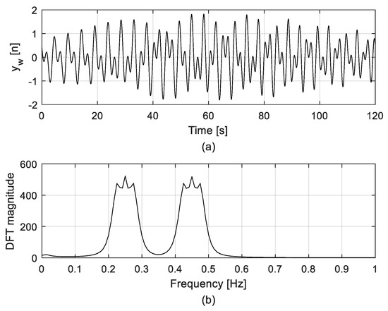
Figure 1. Synthetic oscillation data of the two modes in the simulation with a 50 dB SNR: (a) oscillation data with an interval of 2 min; (b) DFT magnitude for data between 0 and 1 Hz.

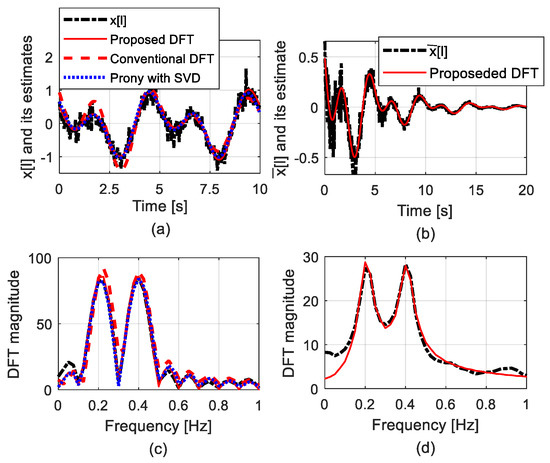
Figure 2. Modal oscillation signal and its estimated signals in the simulation with a 10 dB SNR: (a) x[l] of the first segment and its estimated signals; (b) $\overline{x}\left[l\right]$ of the first two combined segments and its estimated signal; (c) DFT magnitudes of the signals in (a); (d) DFT magnitudes of the signals in (b).

The ESRs of the three methods were calculated in the simulation and are shown in Figure 3a,b for 50 and 10 dB SNRs, respectively. Estimates of the modal oscillation frequencies and damping factors are plotted in Figure 4 and Figure 5 for 50 and 10 dB SNRs, respectively. The ESR of the proposed method improved significantly compared to that of the conventional DFT-based method. Through simulations on a variety of SNRs, it was confirmed that ESRs of the proposed method were similar to or higher than those of the Prony method when the SNR was lower than 10 dB. This results from performing the curve-fitting in the DFT-based method on a small frequency region around each modal peak frequency, where the SNR was relatively higher than other frequency regions. In the case of the SNR higher than 10 dB, ESRs of the Prony method were higher than those of the proposed method, which was due to the fact that the exponential window function weakens modal oscillations in $x\left[l\right]$.

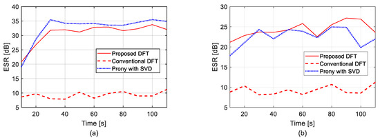
Figure 3. ESRs of the three methods in the simulation: (a) 50 dB SNR; (b) 10 dB SNR.

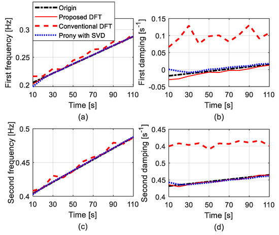
Figure 4. Estimated modal parameters in the simulation with a 50 dB SNR: (a) oscillation frequency of the first mode; (b) damping factor of the first mode; (c) oscillation frequency of the second mode; (d) damping factor of the second mode.

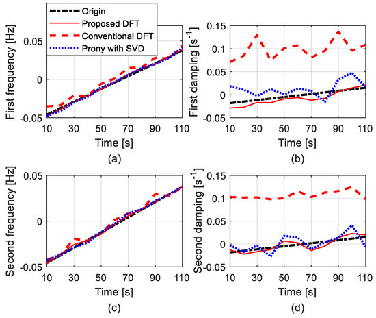
Figure 5. Estimated modal parameters in the simulation with a 10 dB SNR: (a) oscillation frequency of the first mode; (b) damping factor of the first mode; (c) oscillation frequency of the second mode; (d) damping factor of the second mode.

To compare the identification accuracy of the three methods through simulations, another synthetic oscillation signal of a synchronous mode was generated as the following for $y\left(t\right)$:

$$y\left(t\right)=0.01\sin \left(11\pi t\right),0\le t\le 20 \left[s\right]$$

(37)

This synchronous mode has an oscillation frequency of $f_1=5.5$ Hz and a damping factor of ${\xi }_1=0$. Synthetic data for modal identification were obtained as $y_w\left[n\right]=y\left[n\right]+w\left[n\right]$, with a sampling interval of $T_s=1/120$. The white Gaussian noise $w\left[n\right]$ was generated to give a 10 dB SNR to $y_w\left[n\right]$. For modal identification, $y_w\left[n\right]$ was split into 20 segments at intervals of $\Gamma =1$ s.

The subsynchronous mode was identified 19 times sequentially from the 20 segments by the three methods, ESRs of which are shown in Figure 6a. Estimates of the modal oscillation frequency and damping factor are plotted in Figure 6b, c. As mentioned in the previous simulation of a 10 dB SNR in Figure 3b, the ESR of the proposed method was also shown to be similar to that of the Prony method in Figure 6a.

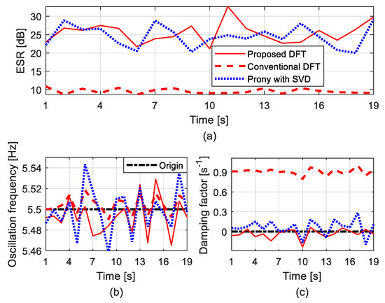
Figure 6. Identification results of the synchronous mode: (a) ESRs of the three methods in the simulation; (b) estimated oscillation frequency; (c) estimated damping factor.

4. Identification of Oscillation modes from PMU Data

4.1. Interarea Mode of Central American Power System

The Central American power system was operated on two islands on July 28, 2012 [5]. The larger island included the power systems of Mexico, Guatemala, El Salvador, and Honduras. The smaller island included the power systems of Nicaragua, Costa Rica, and Panama. Undamped active power oscillations between Guatemala and El Salvador started to occur right after the synchronization of the two networks. The Guatemalan wide-area protection scheme (WAPS) issued a trip command to open the interconnection between Guatemala and El Salvador. Data of an active power flow from the Guatemala Este substation to the Moyuta substation in Guatemala was acquired through a PMU with a measurement rate of 30 per second and are plotted in Figure 7a, where modal oscillations start at 9.3 s and subside after the interconnection opening time of 54.3 s. These active power data were filtered with the Butterworth bandpass filter for rejection of a DC component. The filtered data $y_w\left[n\right]$, $0\le n<1350$, are shown in Figure 7b, where 0 s in the time axis is 9.3 s in Figure 7a. The DFT magnitude of $y_w\left[n\right]$ is shown in Figure 7c, wherein there is a peak of an interarea mode at around 0.2 Hz.

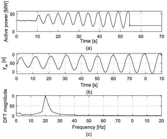
Figure 7. Modal oscillations in the active power of the Central American power system: (a) PMU data; (b) oscillation data for modal identification; (c) DFT magnitude of the oscillation data.

For modal identification, $y_w\left[n\right]$ from 0 to 40 s was split into four segments at intervals of $\Gamma =10$ s. The interarea mode was identified three times sequentially using the four segments of $y_w\left[n\right]$ with the three methods. Figure 8 shows identification results of the first segment, where $x\left[l\right]$ and its estimated signals are plotted in Figure 8a, and their DFT magnitudes are plotted in Figure 8c. The $\overline{x}\left[l\right]$ of the first two combined segments and its estimated signals are plotted in Figure 8b and their DFT are plotted in Figure 8d. Estimated oscillation frequencies and damping factors of the interarea mode are plotted in Figure 9, which shows that the estimates in the proposed method are similar to those in the Prony method, but the estimates of damping factor in the conventional DFT-based method are significantly different from those in the two other methods, as shown in Figure 9b. This implies that the Prony and proposed methods yielded reliable identification results.

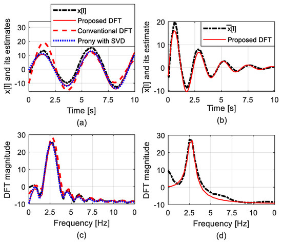
Figure 8. Modal oscillation signal and its estimated signals in the Central American power system: (a) $x\left[l\right]$ of the first segment and its estimated signals; (b) $\overline{x}\left[l\right]$ of the first two combined segments and its estimated signal; (c) DFT magnitudes of the signals in (a); (d) DFT magnitudes of the signals in (b).

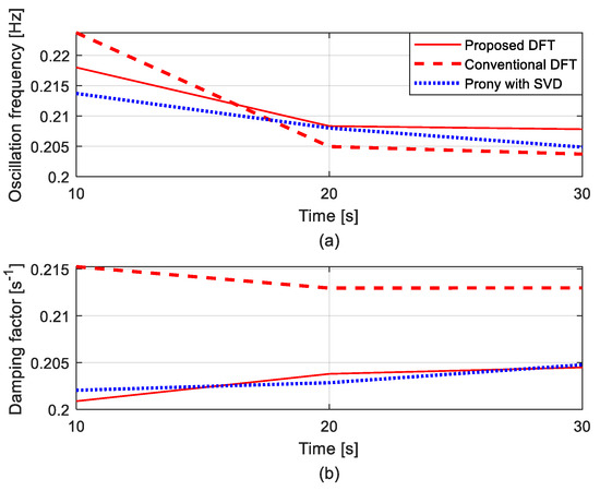
Figure 9. Estimated modal parameters of the Central American power system: (a) oscillation frequency of the interarea mode; (b) damping factor of the interarea mode.

4.2. Regional Mode of New England Power System

The New England power system is in the northeastern part of the Eastern Interconnection in USA. Oscillations with a significant MW magnitude were observed in multiple locations of the New England power system on July 20, 2017. A regional mode of 1.13 Hz was engaged in the oscillations, whose data were acquired from Line 2 at substation 2 through a PMU with a measurement rate of 30 per second [6]. PMU frequency data obtained at a 3-min interval for the oscillations are plotted in Figure 10a, for which oscillation data for modal identification were extracted from 70 to 110 s. These frequency data were filtered with the Butterworth bandpass filter for rejection of a DC component. The filtered oscillation data $y_w\left[n\right]$, $0\le n<1200$, are plotted in Figure 10b, where 0 s in the time axis corresponds to 70 s in Figure 10a. The DFT magnitude of $y_w\left[n\right]$ is plotted in Figure 10c, which shows a peak for the regional mode at around 1.13 Hz.

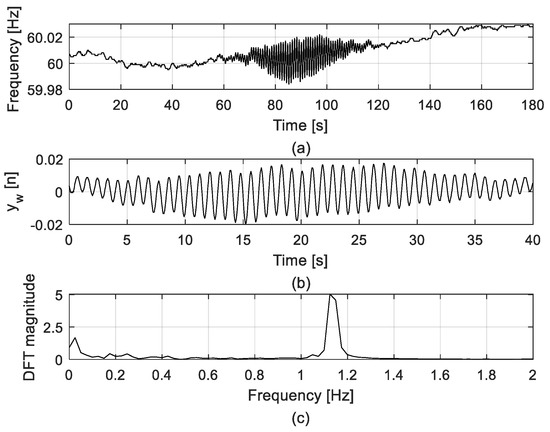
Figure 10. Modal oscillations in the system frequency of the New England power system: (a) PMU data; (b) oscillation data for modal identification; (c) DFT magnitude of the oscillation data.

For modal identification, $y_w\left[n\right]$ was split into 16 segments at intervals of $\Gamma =2.5$ s. The regional mode was identified 15 times sequentially using the 16 segments of $y_w\left[n\right]$ in the three methods. $x\left[l\right]$ and its estimated signals of the first segment are plotted in Figure 11a, and their DFT magnitudes are plotted in Figure 11c. $\overline{x}\left[l\right]$ of the first two combined segments and its estimated signals are plotted in Figure 11b and their DFT are plotted in Figure 11d. The estimated oscillation frequencies of the three methods are shown to be similar in Figure 12a. The estimated damping factors in the Prony and proposed methods are similar to each other, but they are significantly different from those in the conventional DFT-based method. This implies that the Prony and proposed methods yielded reliable identification results.

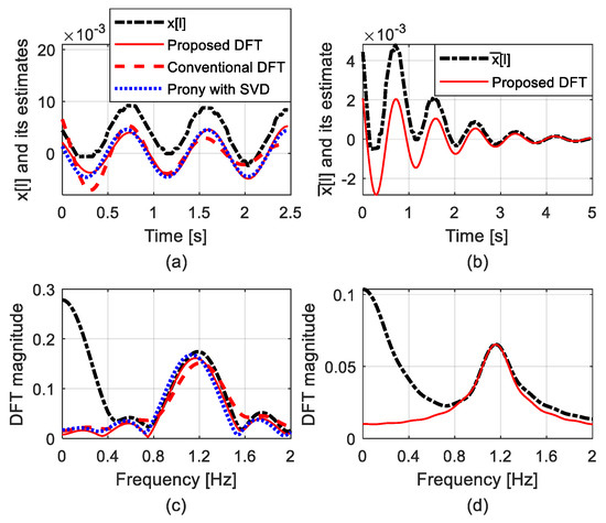
Figure 11. Modal oscillation signal and its estimated signals in the New England power system: (a) $x\left[l\right]$ of the first segment and its estimated signals; (b) $\overline{x}\left[l\right]$ of the first two combined segments and its estimated signal; (c) DFT magnitudes of the signals in (a); (d) DFT magnitudes of the signals in (b).

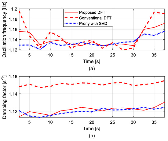
Figure 12. Estimated modal parameters of the New England power system: (a) oscillation frequency of the regional mode; (b) damping factor of the regional mode.

5. Conclusions

In this paper, a DFT-based method with an exponential window function has been proposed to identify oscillation modes from segments of modal transient data which involve a long duration with a nonstationary trend. The proposed method overcomes the limited use of the conventional DFT-based method, which cannot be applied efficiently to such segment data. Through simulations on synthetic oscillation data, it was shown that the identification accuracy of the proposed method was significantly improved compared to the conventional DFT-based method. In the simulations, when the SNR was below 10 dB, the identification accuracy of the proposed method was not lower than that of the Prony method. The proposed method can be applied effectively to low-SNR PMU data, which can be acquired on noisy transmission grids, distribution grids, and microgrids. The feasibility of the proposed method was verified by identifying real-world oscillation modes from PMU data, where the proposed and Prony methods yielded similar estimates of modal parameters.

References

- Kundur, P. Power System Stability and Control; McGraw-Hill: New York, NY, USA, 1994. [Google Scholar]
- Bahrman, M.; Larsen, E.V.; Piwko, R.W.; Patel, H.S. Experience with HVDC-turbine-generator torsional interaction at Square Butte. IEEE Trans. Power App. Syst. 1980, 99, 966–976. [Google Scholar] [CrossRef]
- Fan, L.; Kavasseri, R.; Miao, Z.L.; Zhu, C. Modeling of DFIG based wind farms for SSR analysis. IEEE Trans. Power Del. 2010, 25, 2073–2082. [Google Scholar] [CrossRef]
- Hauer, J.; Trudnowski, D.; Rogers, G.; Mittelstadt, B.; Litzenberger, W.; Johnson, J. Keeping an eye on power system dynamics. IEEE Comput. Appl. Power 1997, 10, 50–54. [Google Scholar] [CrossRef]
- Espinoza, J.V.; Guzman, A.; Calero, F.; Mynam, M.V.; Palma, E. Wide-Area Protection and Control Scheme Maintains Central America’s Power System Stability. In Proceedings of the Saudi Arabia Smart Grid Conference, Jeddah, Saudi Arabia, 14–17 December 2014; pp. 1–9. [Google Scholar]
- Test Cases Library of Power System Sustained Oscillations. Available online: http://web.eecs.utk.edu/~kaisun/Oscillation/actualcases.html (accessed on 13 August 2019).
- Rauhala, T.; Gole, A.M.; Jarventausta, P. Detection of subsynchronous torsional oscillation frequencies using phasor measurement. IEEE Trans. Power Syst. 2016, 31, 11–19. [Google Scholar] [CrossRef]
- Jamei, M.; Scaglione, A.; Roberts, C.; Stewart, E.; Peisert, S.; McParland, C.; McEachern, A. Anomaly detection using optimally placed μPMU sensors in distribution grids. IEEE Trans. Power Syst. 2018, 33, 3611–3623. [Google Scholar] [CrossRef]
- Karim, M.A.; Currie, J.; Lie, T.-T. Dynamic event detection using a distributed feature selection based machine learning approach in a self healing microgrid. IEEE Trans. Power Syst. 2018, 33, 4706–4718. [Google Scholar] [CrossRef]
- Hwang, J.K.; Liu, Y. Identification of interarea modes from an effectual impulse response of ringdown frequency data. Electric Power Systems Research 2017, 144, 96–106. [Google Scholar] [CrossRef]
- Crow, M.L.; Singh, A. The matrix pencil for power system modal extraction. IEEE Trans. Power Syst. 2005, 20, 501–502. [Google Scholar] [CrossRef]
- Rios, M.A.; Ordonez, C.A. Online electromechanical modes identification using PMU data. In Proceedings of the IEEE Grenoble PowerTech, Grenoble, France, 16–20 June 2013; pp. 1–6. [Google Scholar]
- Hwang, J.K.; Liu, Y. Identification of interarea modes from ringdown data by curve-fiting in the frequency domain. IEEE Trans. Power Syst. 2017, 32, 842–851. [Google Scholar]
- Hwang, J.K. Parametric DFT identification of interarea modes in consideration of a decaying DC. In Proceedings of the IEEE PES General Meeting, Boston, MA, USA, 17–21 July 2016; pp. 1–5. [Google Scholar]
- Hauer, J.F.; DeSteese, J.G. A Tutorial on Detection and Characterization of Special Behavior in Large Electric Power Systems; Pacific Northwest National Laborartory: Cambridge, MA, USA, 2004; PNNL-14655. [Google Scholar]
- Pierre, J.W.; Trudnowski, D.J.; Donnelly, M.K. Initial results in electromechanical mode identification from ambient data. IEEE Trans. Power Syst. 1997, 12, 1245–1251. [Google Scholar] [CrossRef]
- Oppenheim, A.V.; Schafer, R.W. Digital Signal Processing; Prentice-Hall: Englewood Cliffs, NJ, USA, 1975. [Google Scholar]
- Larsson, M.; Laila, D.S. Monitoring of inter-area oscillations under ambient conditions using subspace identification. In Proceedings of the IEEE PES General Meeting, Calgary, AB, Canada, 26–30 July 2009; pp. 1–6. [Google Scholar]
- Anderson, P.M.; Mirheydar, M. A low-order system frequency response model. IEEE Trans. Power Syst. 1990, 5, 720–729. [Google Scholar] [CrossRef]
- Lin, X.; Weng, H.; Zou, Q.; Liu, P. The frequency closed-loop control strategy of islanded power systems. IEEE Trans. Power Syst. 2008, 23, 796–803. [Google Scholar]
- Qi, L.; Woodruff, S.; Qian, L.; Cartes, D. Prony analysis for time-varying harmonic. In Time-Varying Waveform Distortions in Power Systems; Ribeiro, P.F., Ed.; Wiley-IEEE Press: Hoboken, NJ, USA, 2009; pp. 317–330. [Google Scholar]
- Xiao, J.; Xie, X.; Han, Y.; Wu, J. Dynamic tracking of low-frequency oscillations with improved Prony method in wide-area measurement system. In Proceedings of the IEEE PES General Meeting, Denver, FL, USA, 6–10 June 2004; pp. 1–6. [Google Scholar]
© 2019 by the authors. Licensee MDPI, Basel, Switzerland. This article is an open access article distributed under the terms and conditions of the Creative Commons Attribution (CC BY) license (http://creativecommons.org/licenses/by/4.0/).