Abstract
Wireless rechargeable sensor networks (WRSNs) have gained much attention in recent years due to the rapid progress that has occurred in wireless charging technology. The charging is usually done by one or multiple mobile vehicle(s) equipped with wireless chargers moving toward sensors demanding energy replenishing. Since the loading of each sensor in a WRSN can be different, their time to energy exhaustion may also be varied. Under some circumstances, sensors may deplete their energy quickly and need to be charged urgently. Appropriate scheduling of available mobile charger(s) so that all sensors in need of recharge can be served in time is thus essential to ensure sustainable operation of the entire network, which unfortunately has been proven to be an NP-hard problem (Non-deterministic Polynomial-time hard). Two essential criteria that need to be considered concurrently in such a problem are time (the sensor’s deadline for recharge) and distance (from charger to the sensor demands recharge). Previous works use a static combination of these two parameters in determining charging order, which may fail to meet all the sensors’ charging requirements in a dynamically changing network. Genetic algorithms, which have long been considered a powerful tool for solving the scheduling problems, have also been proposed to address the charging route scheduling issue. However, previous genetic-based approaches considered only one charging vehicle scenario that may be more suitable for a smaller WRSN. With the availability of multiple mobile chargers, not only may more areas be covered, but also the network lifetime can be sustained for longer. However, efficiently allocating charging tasks to multiple charging vehicles would be an even more complex problem. In this work, a genetic approach, which includes novel designs in chromosome structure, selection, cross-over and mutation operations, supporting multiple charging vehicles is proposed. Two unique features are incorporated into the proposed algorithm to improve its scheduling effectiveness and performance, which include (1) inclusion of EDF (Earliest Deadline First) and NJF (Nearest Job First) scheduling outcomes into the initial chromosomes, and (2) clustering neighboring sensors demand recharge and then assigning sensors in a group to the same mobile charger. By including EDF and NJF scheduling outcomes into the first genetic population, we guarantee both time and distance factors are taken into account, and the weightings of the two would be decided dynamically through the genetic process to reflect various network traffic conditions. In addition, with the extra clustering step, the movement of each charger may be confined to a more local area, which effectively reduces the travelling distance, and thus the energy consumption, of the chargers in a multiple-charger environment. Extensive simulations and results show that the proposed algorithm indeed derives feasible charge scheduling for multiple chargers to keep the sensors/network in operation, and at the same time minimize the overall moving distance of the mobile chargers.
1. Introduction
In wireless sensor networks (WSN), hundreds or thousands of homogenous sensors with limited battery power are deployed in the region where information will be collected. Sensor nodes detect their proximate environment for specific information and send that information to a base station. While sensors are deployed uniformly in a wireless sensor network, sensors located in different positions bear different communication responsibilities. Accordingly, the energy consumption of sensors in the network may be heterogeneous, so some may drain their power earlier than the others and cause subsequent network failure.
Fortunately, as a result of advances in wireless charging technology [1], it is now possible to recharge the sensors through a vehicle equipped with a charger (will be referred to as mobile charger hereafter) [2,3,4]. WSNs that possess such a recharging capability, which are called wireless rechargeable sensor networks (WRSNs), may potentially extend their network life time. However, the scheduling of recharges needs to take the dynamic change in loading of each sensor, which usually comes in bursts when events occur, into consideration. Otherwise part of the sensors may deplete their energy before being charged, thus resulting in possible network failure. In other words, an efficient scheduling of mobile charger(s) to perform its/their duty has/have to consider varied sensor requirements. Note that, regardless of the number of mobile chargers used in a WRSN, optimal charging scheduling and its related issues have been proven to be an NP-hard problem and so far only heuristic/near-optimal solutions can be provided.
Two essential factors that are often used to determine the order of recharge are time (the sensor’s deadline for recharge or energy consumption rate) and distance (from charger to the sensor demands recharge) [5,6]. The two factors have usually been combined together through some pre-determined weights in previous works. For example, in reference [5], both factors are considered equally, while reference [6] argues that a 100% (time, in terms of energy consumption rate, which is not constant as reference [5] assumes) and 80% (distance) split would be more favorable. However, as we have stated earlier, in a dynamic changing sensor network environment, it is questionable whether any static combination of the two parameters will meet all the sensors’ charging requirements.
Accordingly, in this work, we propose a genetic approach to solve the emergent charging scheduling problem. The proposed algorithm is unique in adopting the following two strategies. First, the genetic optimization process incorporates the Earliest Deadline First (EDF) and Nearest Job First (NJF) scheduling outcomes into the initial chromosome population, which guarantees that the results of the genetic optimization would be no worse than the EDF and NJF results. More importantly, it also implies that both the time and distance (encoded in chromosomes based on EDF and NJF generated outcomes) factors in charge scheduling are taken into consideration, while the genetic process is used in some way to derive the weightings of the two. Secondly, the proposed algorithm may assign the charging tasks to single or multiple chargers to meet the in-time charging limitations. In the case of a multiple-charger arrangement, a clustering step is applied prior to every chromosome re-generation procedure. The clustering process proceeds by grouping neighboring sensors that demand recharges so that each group may be assigned to one of the available chargers, which thus confines the movement of each mobile charger in a more local region. The advantages of the above two strategies, as will be shown later in the simulation results, are improving the successful sensor recharge rate and greatly shortening the overall moving distance of mobile chargers. In other words, the charging need of sensors can be addressed, while reducing the energy consumption of mobile chargers. In addition, the proposed algorithm is generic as it makes no assumption regarding what target power level (i.e., charging deadline) sensors may issue charging requests and poses no restriction to both a charging vehicle’s moving speed and a sensor’s charging rate. However, the issue with genetic process is that scheduling may need a more powerful platform as compared to the method used in reference [5].
Overall, the objective of this research is to develop an effective genetic-based scheduling algorithm to sustain the lifetime of sensor networks in a multi-charger (include single charger) context. The novel design of chromosome structure, selection, cross-over and mutation operations, together with the afore-mentioned two strategies to fulfill the above goal will be presented and implemented. Extensive simulations with parameters setting that is as realistic as possible will be conducted to evaluate the performance of the proposed genetic approach, the effectiveness of incorporating one or both of the strategies, and the effects of the number of mobile chargers. Performance comparisons will also be made among ours and the other similar implementations. Note that a preliminary idea for this work appeared in reference [7].
The rest of the paper is organized as follows. In the related work section, we review previous works in the field of rechargeable wireless sensor networks. The proposed genetic approach to solve the charging scheduling problem is provided in the following section. Extensive simulation results of the proposed approach will be described and discussed in the simulation results and discussions section. Finally, we conclude this paper and list possible future research directions in the final section.
2. Related Works
Wireless sensor networks have received a lot of attention and have been widely used in collecting data in various fields in the past two decades [8]. However, energy drain due to the limited battery power of the sensor nodes has been one of the major issues that results in eventual network failure. However, the energy of sensors can be replenished by collecting ambient energy, such as solar power, vibration energy, and so on. Nevertheless, the energy that can be harvested is unstable and unpredictable. Fortunately, the feasibility of wireless power transfer through magnetic resonance, as demonstrated by Kurs et al. [1], makes sustainable wireless sensor networks possible. Accordingly, a WSN that possesses such a battery recharge capability, the Wireless Rechargeable Sensor Network (WRSN) has emerged to become one of the popular areas in current WSNs research [9,10,11].
Some research proposed to use static charging devices to charge the sensors [12,13]. The required number of charging devices may be increased proportionally to the area of the wireless sensor network, which induces more cost. Moreover, due to the limited range of wireless power transmission, the static charger solution may not be as energy efficient as compared to the mobile charger solutions [14].
In terms of mobile charger solutions, single or multiple charging vehicle(s) may be used. The former may work well in a small scale environment [15]. Yet, in a larger network, one mobile charger may not be feasible, considering the limited amount of energy it can carry. However, in both cases, one of the most essential issues is to schedule the mobile charger(s) so that it/they can charge whichever sensor that is running out of energy in time to keep the network operating.
L. Fu et al. [16] proposed an energy synchronized mobile charging (ESync) protocol, which simultaneously reduces both of the charger’s travel distance and the charge waiting time of sensor nodes. Their algorithm operates by constructing a set of nested TSP (Travelling Salesman Problem) tours, which is an NP-hard problem, based on the sensor nodes’ energy consumption rate. Sensor nodes are grouped according to their power consumption rate and charger is scheduled to visit nodes belonging to the group in the order of descending consumption rate. However, the possible issue with this technique would be that scheduling has to be redone once the power consumption rate of the sensors changes, which happens quite often when new events spotted in the network.
L. Xie et al. [17] showed that WSN can remain operational forever through periodic wireless energy transfer. They assumed that the node’s energy consumption is fixed. After careful analysis, the near optimal charging schedule is obtained. The same team [18] also proposed to exploit the multi-node wireless energy transfer technology provided by magnetic resonant coupling. Their algorithm partitions a two-dimensional plane into adjacent hexagonal cells, and the charging vehicle visits these cells and charges multiple sensor nodes from the center of a cell. They then pursue a formal optimization framework by jointly optimizing the traveling path, flow routing and charging time. The result was a provably near-optimal solution for any desired level of accuracy. Both techniques mentioned above work on finding the (near) optimal traveling paths for mobile charger so that it may visit and charge sensor nodes periodically. In other words, the issue of on-demand recharging requirements of sensors was not addressed.
Y. Shu et al. [19] proposed to control the velocity of mobile chargers in order to reduce the traveling time of chargers so that effective time spent on sensors charging can be increased. They first proved that velocity control of mobile charger in the specified problem to be NP-hard, and then developed a heuristic solution with a provable upper bound. Although the work does not relate directly to the recharge scheduling problem, yet it indicates a potential factor to be considered in future research.
M. Pan et. al. [20] proposed a heuristic algorithm to solve the charging problem. In their method, the charging vehicle not only charges the sensors, but also collects data from some sensors acting as intermediate sinks and then brings back the information to the base station. The goal is to reduce the propagation of data packets among sensor nodes, which is the primary source of energy consumption. This appears to be a good idea, since reducing the energy consumption of sensors relieves the burden of chargers, which may deserve further attention in our future study. However, on-demand recharging requirement of sensors was still not addressed in their work.
Jie Jia et al. [21] used a heuristic algorithm to locate sensors that need charging, followed by a genetic approach to find a shorter moving sequence. The proposed strategy used only one mobile charger, but the authors did not discuss how to fulfill the dynamic requirements of sensors. A.H. Mohamed [22] also adopted a genetic algorithm to the charging vehicle scheduling problem. They used a cluster structure to decrease the complexity of a genetic algorithm. That is, their algorithm finds a better moving path among cluster heads only. The mobile charger charged the cluster heads, which then charged their members in the cluster hierarchy via energy propagation. The advantage of such a hierarchical design would thus be reducing the traveling distance of the mobile charger. However, the possibility of using multiple charging vehicles and dynamic charging requirements was not included in their research scope.
H. Dai et al. [15] proved that the optimal quantity of the charging vehicles in the wireless sensor network is an NP-hard problem, and they use an approximation approach to obtain a better solution. The authors proposed a heuristic approach to get the minimal number of charging vehicles to keep the residual energy of sensors above some working threshold. In their work, the energy consumption of each sensor is assumed to be uniform and constant, which under many circumstances may not be true. In other words, the diversity of sensor requirements should be taken into consideration in charging scheduling. Moreover, the efficient use of the charging vehicles to address the dynamic charging requests is not included in their research.
According to the aforementioned prior research, with either one charger or multiple chargers, the optimal charging scheduling and its related issues, have either been proven to be an NP-hard problem [15,16,18] or only heuristic/near-optimal solutions can be provided [18,20,21,22]. Accordingly, in this paper, a genetic approach like Jie Jia et al. [21] and A.H. Mohamed [22] is adopted. However, the scheduling problem will be addressed in the context of multiple mobile chargers and the dynamic sensors charging requirement will also be taken into consideration. In addition, meeting the recharging requirements of sensors while reducing the travelling distance is also one of the major issues that was addressed [16,19], which will be a major point in our proposed solution as well.
3. Genetic Approach for Multiple Mobile Chargers Scheduling
In this section, the proposed genetic approach for scheduling multiple mobile chargers in WRSN is presented, followed by the context and assumptions of the proposed approach, and the algorithm details.
First of all, assume that there are a total of Ncar mobile chargers and the positions of sensors are already known to the base station (BS). In addition, a sensor node will send a recharge request to the BS when its battery power drops to some predefined threshold, which means the BS is also aware of the residuals of the sensor, i.e., its remaining work time (RWT). All sensor nodes, together with their remaining work time and positions, that demand charging are kept in the charging_list. With the above information, the BS may determine when to initiate a charge scheduling and determine the charging routes for the mobile chargers. The goal is to minimize the moving distance of the chargers while meeting the requirement that all sensors are recharged in time if possible. Specifically, when the BS finds the “start of charge scheduling” condition (as described later) occurs, it initiates the scheduling procedure (a genetic algorithm as described later in this section) and then assigns missions to the mobile chargers accordingly.
3.1. Conditions for Start of Charge Scheduling
The preliminary requirement to meet the “start of charge scheduling” condition is the availability of mobile charger(s). In other words, there must be at least one (out of ) charger available at BS’s disposal. The number of available chargers is denoted as , In case ≥ 1, either one of the following two scenarios: (1) the number of sensor nodes demanding charging reaches the capacity of recharging (Q) that currently available chargers can provide, or (2) the minimum recharging deadline time, min_RDT, beyond that some sensor nodes may die if a charging mission does not start, which will trigger the initiation of a charge scheduling procedure.
The capacity of charging, Q, is the total number of sensor nodes that can be charged given a specific number of available chargers. It may be estimated according to the total battery power required by the sensors and the battery power may be provided by the available charging vehicles. To simplify the matter, let us assume that each charging vehicle is capable of charging an equal number of sensor nodes, . In case there are chargers, Q can be expressed by Equation (1).
The minimum recharging deadline time (min_RDT), can be computed as follows. First, sort the charging tasks demanded by sensor nodes in the charging_list according to the Earliest Deadline First (EDF) order [23] and distribute these tasks evenly to all available mobile chargers. The arrival time, , of each charger to each assigned sensor node, , can be calculated given the facts that visiting order, distance to sensor node and moving speed of mobile charger are known. The estimated recharging deadline time for sensor node , can be derived by computing the difference between the arrival time (of mobile charger) and its remaining work time, as depicted in Equation (2).
To deriving the minimum recharging deadline time (min_RDT) is then equivalent to finding the minimum among all the ,
3.2. The Proposed Genetic Charge Scheduling Algorithm
The proposed genetic scheduling algorithm starts by randomly generating initial population P. After an iteration (and every subsequent iteration) of the genetic process, the best α% chromosomes in the population are preserved for the next generation. Also, β% chromosomes of the new population are newly and randomly generated as done in the initial phase. The remaining chromosomes of the new population (1−α%−β%) are generated by using the crossover function from two randomly selected chromosomes of previous generation, among which some might be mutated with γ probability. The genetic process would proceed until it reaches a pre-determined maximum iteration count (max_Iteration) or the fitness function has not been further improved for t consecutive iterations. The detailed genetic algorithm is listed in Algorithm 1. Note that Algorithm 1 would be performed n times with parameter Number_of_car iterates from 1 to n, where n equals to the number of charging vehicles available at the moment when the algorithm starts. The goal is finding the number of charging vehicles (k, ) that achieves the best recharge scheduling.
| Algorithm 1. Genetic algorithm for recharging scheduling |
| Input:Number_of_car, charging_list Output: the best chromosome for recharging scheduling using Number_of_car vehicles 1 Generating initial population P. 2 Select the first chromosome from P to be the best_one chromosome 3 fitness_unchanged_count = 0 4 for i = 0 to max_Iteration do 5 Calculating fitness value of each individual in P 6 Sorting P ascendingly according to the values of individuals 7 Select the first chromosome from P to be the new_best_one chromosome 8 if best_one is equal to new_best_one 9 fitness_unchanged_count ++ 10 else 11 Set best_one to be the new_best_one chromosome 12 fitness_unchanged_count = 0 13 end 14 if fitness_unchanged_count > t 15 Return the best_one chromosome 16 end 17 Set population next_P to {} 18 Add first α% individuals in P to next_P 19 Generate and add β% new individuals to next_P by using Algorithm 2 20 for j = 0 to Population_size·(1−α%−β%) do 21 Select two parents and from P by using Algorithm 3 22 Cross with by using Algorithm 4, and produce child p’ 23 Cross with by using Algorithm 4, and produce child p” 24 Choose the better one from p’ and p” to be 25 Mutate by using Algorithm 5 with probability γ 26 Add into next_P 27 next j 28 next i 29 Return the first chromosome of P |
In the following, the design and generation of chromosomes (Algorithm 2), fitness function, selection (Algorithm 3), crossover (Algorithm 4), and mutation (Algorithm 5) operations that are involved in the afore-mentioned genetic scheduling algorithm will be presented in more detail.
3.2.1. Chromosome Design and Generation
Assume that there are m sensors that need to be recharged in the entire wireless sensor network. In the case of single mobile charger, a chromosome may be designed to contain m genes, with each gene assigned the serial number of the sensor. In other words, a chromosome and a gene represent the list of sensors demand charging and the sensors ID in that list, respectively. The position of gene in a chromosome stands for the charging order of a sensor. Figure 1 depicts a possible gene combination of a chromosome in the case of seven sensors requesting a recharge. In this specific case, sensor 1 would be charged first, followed by sensors 5, 3, 2, 7, 6, and 4.
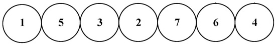
Figure 1.
A sample chromosome.
To allocate the charging tasks to multiple mobile chargers, the assignment of sensors to the charging vehicles should also be included in the chromosome. Accordingly, each gene now contains not only the serial number of a sensor, but also the serial number of the charger that is responsible for recharging of that specific sensor. Figure 2 shows a scenario with 3 chargers and 7 sensors waiting to be recharged. The charging order is {1, 5, 3, 2, 7, 6, 4} and chargers 1, 2, and 3 are assigned to charge sensors {1, 2, 7}, {5, 6}, and {3, 4}, respectively. In that case, the chromosome encoding is depicted in Figure 2.
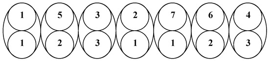
Figure 2.
A sample chromosome for solving the charge scheduling problem with multiple chargers.
Algorithm 2 shows the detailed process of chromosome generation. Note that, assigning adjacent sensors demand recharging to the same charger may be an effective way to reduce the energy cost of moving chargers back and forth among sensors located apart from each other for their missions. To explore and incorporate this idea into our proposed method, we adopt a notion of clustering that is similar to the k-center algorithm. To be more specific, in case there are k available chargers and m to-be-charged sensor nodes, this process may divide these sensors into k groups based on their locality and assign them to the k available chargers. Taking the scenario depicted in Figure 3 as an example, the clustering process proceeds as follows: (1) Calculate the angle, θi (), of the ray originating from BS to each sensor node i (as the θ shown in Figure 3a, ). (2) Sort θi in ascending order and derive the sensor nodes list {7, 6, 5, 4, 3, 2, 1, 8}, which may be considered as a circular queue (3) Pick randomly a sensor from the list as the starting node and assigned sensors evenly to each available chargers. For example, if the second node, 6, is selected, the assignment would go like: {6, 5, 4}→charger 1, {3, 2, 1}→charger 2, and {8, 7}→charger 3, as shown in Figure 3b.
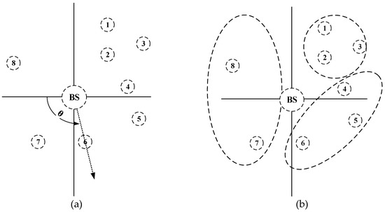
Figure 3.
A scenario depicting how the clustering process in Algorithm 2 works. (a) Calculation of the angle of the ray originating from BS to the sensors. (b) Grouping and assigning sensors to be charged to mobile chargers.
| Algorithm 2. Algorithm for generating chromosome instances |
| Input:Number_of_available_car, charging_list Output: a randomly generated chromosome Chrom 1 Sort sensors in the charging_list in ascending order by the angle of the ray originating from BS to the sensors to be charged and derive new charging _list in angle sequence. 2 Set Chrom = {} 3 = size of charging_list 4 5 for i = 1 to Ncharging_list 6 Set gene.node_id to a randomly selected sensor ID from charging_list 7 Mark gene.node_id in charging_list as used 8 Set angle_seq as the position of gene.node_id in charging_list 9 Set gene.car_id = 10 Add gene to Chrom 11 next i 12 Return Chrom |
3.2.2. Fitness Function
The goal of the proposed charge scheduling algorithm is to charge all the sensors before their batteries exhausted and to minimize the energy consumption of the mobile charger. From the point of view of charging vehicles, the amount of power required for a charging mission does not change no matter what the charging sequence is. Accordingly, minimizing the moving distance of the mobile charger(s) corresponds to saving its/their energy. Before going further with our discussion, a summary of the notations to be used later is listed in Table 1.

Table 1.
Notations used in this work.
In case of using a single charger, the fitness function is designed to be the moving distance of the charger. Since the charging vehicle departs from the base station for charging, and returns to the base station after completing its tasks, the fitness function for some charging path : , , , …, containing n sensors is defined as follows.
The objective is to minimize
We have
where
and
Since each sensor sends its charging request to the base station with the estimated remaining working time , the base station can get the by summing and .
For every node i in charging path , we have
While there are m charging vehicles available with m charging paths : , , , …, (), the fitness function has to take into consideration the sum of all charging vehicles’ moving distance. Similar to Equation (4), the is defined below.
Fitness function for a chromosome x is modified as follows.
Equations (5)–(7) are modified as follows.
So the problem can be formulated as a linear programming formula as follows:
Objective function:
Note, only the scenarios where the charging vehicles move at constant speed and charge sensors at the same rate will be considered in the following discussions. But according to equations above (i.e., Equations (12) and (13)), there is no restriction on both the charging vehicle’s moving speed and the sensor’s charging rate. In addition, sensors can issue requests at different target power levels and provide different charging deadline. As a result, the fitness function as designed and presented above can potentially deal with dynamic sensors’ charging requirements with multiple mobile chargers, which may be an interesting problem to be addressed in the future.
In addition, the charging time should also be included in the fitness function. A schedule that cannot complete the charging tasks is given a larger fitness value so that this schedule has lower possibility of being selected. On the other hand, for charging schedules that can complete charging tasks in time should be given scores according to the times they needed for these tasks. Finally, the fitness function is defined as follows.
The constants a, b, c used in Equation (15) are predefined constant values as the weights of , and , respectively. In the simulations performed in this work, a is set to a very larger number (e.g., 1,000,000) to avoid adopting charging schedules that are not able to fulfill their missions. On the other hand, b and c are both set to 1 for simplicity. In the future, it may be possible to explore various combinations of these three parameters to potentially improve scheduling performance.
3.2.3. Selection
In order to ensure that better chromosomes may possess higher probabilities of being selected to generate new chromosomes, the chromosome pool is first sorted in ascending order according to the fitness values (smaller fitness value implies better chromosome, which would be placed at the forepart of pool). Assume that there are n chromosomes in the pool. Then a random number s is selected from 0 to n2 − 1 and the (n − ⌊⌋)-th chromosome would be selected. To sum up, the algorithm to select a chromosome from the chromosome pool is listed below.
| Algorithm 3. Algorithm for randomly selecting a chromosome |
| Input: an integer number n Output: a chosen chromosome 1 Select a uniformly distributed random number s from 0 to n2−1 2 Choose the (n − ⌊⌋)-th chromosome from the sorted chromosome pool to be the selection result |
3.2.4. Crossover
Crossover proceeds by first randomly selecting two chromosomes Ca and Cb from the chromosome pool using the selection method mentioned above (Algorithm 3). A cutting point k is then randomly generated. Let C[i] represent for the gene at position i of chromosome C, and C[i, j] represents a subsequence of genes of chromosome C from the position i to j. Then the content of the crossover chromosome Cc is composed of Ca[0, k − 1] and Cb[k, n − 1]. However, since the contents of Ca[0, k − 1] and Cb[k, n − 1] may be duplicated, the crossover steps are modified accordingly as follows.
| Algorithm 4. Algorithm for chromosomes’ crossover |
| Input: Two chromosomes Ca and Cb. Output: A new chromosome Cc 1 Randomly select an integer k, where . 2 Set Cc [0, k − 1] = Ca [0, k − 1]. 3 Set where 4 Find the elements from Cb that have not yet been placed in Cc, and fill them sequentially to the positions marked with −1 in Cc. |
For example, a possible crossover process, as depicted in Algorithm 4, of two chromosomes, Ca and Cb, with each containing 5 genes and with cutting point k being set to 3 is shown in Figure 4. As can be seen, the crossover result, Cc, receives its first 3 (=k) and last 2 genes from Ca and Cb, respectively. However, since the two genes from Cb contain sensor IDs that have overlapped with the ones from Ca, they would be marked with −1 and later been replaced with ones that are not shown in genes from Ca, which would be sensor ID 4 and 5.
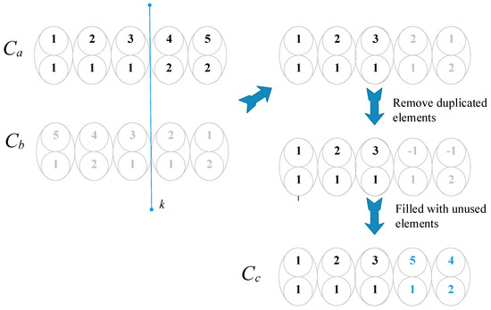
Figure 4.
An illustration of the crossover operation.
3.2.5. Mutation
As a chromosome should contain each sensor to be charged just once, a sensor ID in a chromosome cannot just change to another one randomly. Thus, the mutation operation is designed to swap the IDs of two randomly selected genes in a chromosome. The algorithm to mutate a chromosome Cm is presented in Algorithm 5 below. Figure 5 is an illustration of the mutation process depicted in Algorithm 5.
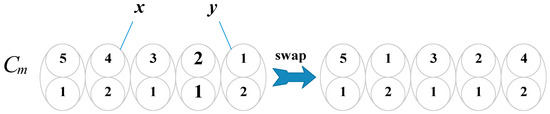
Figure 5.
An illustration of the mutation operation.
| Algorithm 5. Algorithm for mutating a chromosome |
| Input: chromosome Cm Output: mutated chromosome Cm 1 Select two distinct number x and y randomly, 0 ≤ x, y ≤ n − 1. 2 Swap the ID values of Cm[x] and Cm[y]. |
4. Simulation Results and Discussions
The simulation program was coded with Visual Studio C# and executed on a personal computer with an Intel i7-8700 CPU running Microsoft Windows 10. The simulation environment is specified by a 1000 × 1000 meters’ rectangular region with 1000 sensors uniformly and randomly deployed. The base station is located at the center of the area. Mobile chargers are equipped with independent and unlimited power source for their movement. Also assume that a gradient based routing tree [24] has been built already. Packets are sent from nodes to the base station hop by hop. Based on the free space model proposed in reference [25], to transmit l bits over d distance would cost and to receive l bits would cost as shown below.
The traffic load of each node is assigned a random value uniformly distributed within range [0, x/n], where n is the total number of nodes. In other words, in every second, each sensor node has a probability in between 0 and x/n in generating a packet. Whenever a node finds that its remaining energy is lower than the preset percentage (Eth), it needs to send the charging request packet to the base station. Both the request packet and the data packet are fixed at a size of 10 kB in the following simulations. Packet transmission is set to 1/100 s for one hop delivery. The content of a charging request packet includes node id, energy consumption rate Rc, residual energy Ec, and demand time Tcurrent. Energy consumption rate Rc and Remaining Work Time (RWT) are calculated using the following equations.
where Efull and Tfull are battery capacity and time that the sensor was last charged.
Unless otherwise specified, the parameters used in simulations are summarized in Table 2. All the results are the average of 100 simulations. Three performance metrics, as listed below, are used for evaluating the simulation results.
Table 2.
Simulation parameter settings.
- Percentage or number of sensors been charged—the percentage of sensors can be successfully charged. This is the primary goal of the proposed algorithm: the more sensors been charged successfully, the longer the network life time would be expected.
- Moving distance—the average moving distance of the charging vehicles in charging a sensor. It is calculated by dividing the total moving distance of charging vehicles by the total number of sensors been charged. The shorter the average moving distance, the lower the cost in charging the sensors.
- Percentage of data packets been delivered—the percentage of all transmitted data packets that are successfully delivered to their destinations.
Note, as shown in Table 3, most of our parameter settings are based on those used by Tsoumanis et al. [26], and three other research articles [5,6,17]. In some cases, the values of our parameters were chosen to be even harsher than theirs. Examples of this were the network traffic, battery power of chargers and sensor nodes’ initial energy power. Also, according to our assessment (through simulation), the energy consumption rate of the free space model is also higher than the other models in our scenario, and thus puts more pressure on the network. Finally, other than the assumption that mobile chargers have an independent and unlimited power source for their movement, all the other parameter settings are chosen so that they are as close as possible to a realistic scenario.
Table 3.
Parameter settings used in other methods.
We have designed and conducted five simulations, with the results shown in the following sub-sections.
4.1. The Impacts of Genetic Algorithm Parameters
The first simulation is designed to assess the two important parameters, population size and maximal number of iterations, of a genetic procedure. To speed up the simulation, the simulation time is limited to 10,000 seconds with network traffic set at [0, 100/n], while the other parameters are the same as shown in Table 2. In these simulations, the values of both the population size and maximal number of iterations are set in between 200 and 800. The following figures show the results of all the three performance metrics listed above plus the average computation time (the average time required for completing a scheduling task on the simulation personal computer) by varying the population size and maximal number of iterations. Figure 6 reveals that increasing the value of population size only slightly improves the percentage of sensors being charged and packets received, and the average moving distance. On the other hand, the increase in maximal number of iterations not only has no apparent impact on the performance, but also greatly prolongs the computation process. This may imply that the genetic algorithm usually converges before it reaches the maximal iteration counts. Thus, in the following simulations, it may be adequate to set the population size and the maximal number of iteration to 200 and 200, respectively.
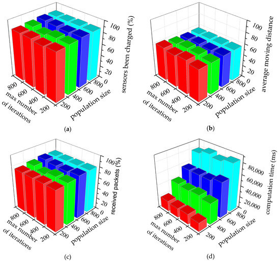
Figure 6.
The performance metrics of the proposed genetic algorithm when varying population sizes and maximal number of iterations. (a) percentage of sensors been charged, (b) average moving distance, and (c) percentage of packets received, and (d) average computation time, vs population sizes and maximal number of iterations. Note that simulation time and network traffic are set at 10,000 s and [0, 100/n], while the other parameters, except population size and maximum number of iterations, are the same as shown in Table 2.
4.2. The Impacts of Vehicle Parameters
The second simulation is to investigate the effects of charging vehicle’s moving speed and sensor charging speed, which determine the cost (in time) of charging tasks. Intuitively, the smaller the time cost, the easier it is to find a feasible solution to complete the charging tasks. As expected, Figure 7a,c show that with a higher vehicle speed and charging rate, it is easier to get charging tasks done, which again improves the packets received rate. Figure 7b shows that when charging tasks can be mostly completed (vehicle speed ≥ 5 m/s and charging rate ≥ 5 J/s), both vehicle speed and charging rate do not have much impact on the average moving distance (of charging vehicles). Accordingly, the following simulations will set the speed of vehicle and battery charging rate to 5 m/s and 5 J/s, respectively.
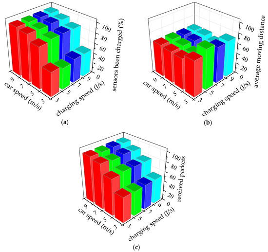
Figure 7.
The performance metrics under different vehicle moving speed and battery charging rate. (a) percentage of sensors been charged, (b) average moving distance, and (c) percentage of packets received, vs moving speed of charging vehicle and charging rate of sensor. Note that simulation time and network traffic are set at 10,000 s and [0, 100/n], while the other parameters, except for vehicle moving speed and sensor charging speed are the same as shown in Table 2.
4.3. The Impacts of Clustering and Incorporation of EDF/NJF Outcomes to Initial Chromosomes
In the following simulation, performance of variations of our proposed genetic scheduling approach is examined. Five possible variations include: implementations with clustering step only (denoted by Clustering), with clustering step plus incorporating EDF and/or NJF scheduling outcomes into the initial chromosome (denoted by EDF-Clustering, NJF-Clustering, and EDF + NJF-Clustering), and with none of the above (denote Random, meaning no clustering is performed and all initial chromosomes are generated randomly).
From the results shown in Figure 8, it is obvious that, when comparing to pure genetic algorithm (Random), the full implementation of all additional steps (EDF + NJF + Clustering, which includes clustering and EDF + NJF) of our proposed algorithm performs significantly better in all three performance metrics. It is also interesting to see the impacts of each extra steps. First of all, clustering alone does not have any physical effect when there is only one charger, which is within our expectations. Clustering only starts to have moderate performance margin over the random genetic implementation in multi-charger scenarios. Second, NJF-Clustering appears to perform better (in terms of successful recharging and data packet delivery rate) than EDF-Clustering in cases with less available chargers. However, as the number of chargers increases (≥3), the performances of the two start going the opposite directions. It appears that when there are more chargers at our disposal, the weighting in “time” is more essential than the “distance” factor. Note, NJF-Clustering does still perform better in terms of average moving distance, which is reasonable as it takes “distance” as its first priority. Third, although EDF + NJF + Clustering implementation consistently achieves less in average moving distance of chargers, it seems to be the only one that this metric increases as the number of cars. The reason for this may be due to the sometimes conflicting circumstances between the “time” and “distance” factors, and the compromise made by the genetic procedure causes the increase in average moving distance.
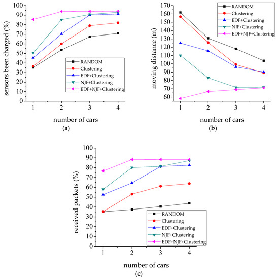
Figure 8.
Performance comparisons among variations of our proposed algorithm in terms of: (a) percentage of sensors being charged successfully, (b) average moving distance of charging vehicles, and (c) percentage of successful data packets delivery. Note that simulation time and network traffic are set at 10,000 s and [0, 100/n], while the other parameters are the same as shown in Table 2.
4.4. The Impacts of Varying Number of Chargers
In this simulation, we try to investigate the effects of increasing the number of chargers under light ([0..10/n]) and heavy ([0..100/n]) network traffic scenarios. Note, the full implementation of our algorithm (i.e., the EDF + NJF + Clustering implementation) is adopted in this and the following simulations. Also, the simulation time is extended to 1,000,000 s to explore the comparatively long-term effects of our algorithm.
As shown in Table 4, we can see that under light traffic conditions, an increase in the number of chargers available does not improve much in terms of both a successful sensor charging rate and data packet delivery rate. On the other hand, it does show a positive impact as network traffic becomes heavier, especially in terms of data packet delivery rate. Note that less than 100% of the percentage of sensors that have been charged may be due to the strict setting in the initial residual of nodes (in-between 5% and 25%) and the hot spot effect around the base station, which result in the early death of nodes without having any chance of being recharged. In addition, we may also observe the results and realize how the failure of even a small percentage of sensors may affect the final successful data delivery. For example, in a scenario with heavy network traffic and one available charger, a less than 4% rate of recharge misses may cause drops in packet delivery by more than a quarter.
Table 4.
Simulation results with varying numbers of chargers.
When it comes to moving distance, more chargers mean more add-on costs induced by moving these chargers back to the base station for energy replenishment, and thus increase the average moving distance of charging vehicles. Overall, having more chargers is definitely helpful in prolonging a sensor network’s operations. However, the average moving distance of chargers in light traffic conditions all appear to be longer. It seems that there are less recharge requests expected in that case. As a result, each scheduled mission of a charger turns out to service less sensor nodes, and thus increases the average moving distance per sensor charged. Also, due to the same afore-mentioned reasons (the strict setting in initial residual of nodes and the hot spot effect around the base station), the chargers (initially located at the base station) usually tend to service nearby sensor nodes in the beginning of the simulation. As the simulation proceeds over time, the effect would be less obvious. That is why we see results with significantly lower average moving distances (less than 100 m) from previous simulations when their simulation time was set to 10,000, instead of 1,000,000 s in this simulation and the following ones.
4.5. Comparison of Scheduling Performance with Other Mrthods
In the final simulation, we compare scheduling performance between ours and the afore-mentioned algorithm [5], which uses static combination of “time” and “distance” with the same weight. The algorithm was called TemporAl and Distantial Priority charging scheduling algorithm (denoted by TADP). EDF scheduling outcomes are also included and used as the baseline for comparison. The simulations are done under both light ([0..10/n]) and heavy ([0..100/n]) network traffic scenarios with one charger. The results, as shown in Table 5, indicate that our algorithm outperforms the other two implementations in all three performance metrics under both network loading conditions.
Table 5.
Performance comparison between ours and the other methods.
One thing that deserves noting is that TADP performs worse than EDF in the lighter traffic condition, and only does slightly better when traffic is heavier. It appears that given “time” and “distance” the same weight as TADP may result in a scenario with a sensor node closer to the charger but with an less urgent need to be recharged first. In the meantime, another sensor that needs immediate attention yet located a few hops away may just drain its last bit of power. On the other hand, EDF would have made a completely different decision, which may just have enough time to save both sensors from dying in a less busy network environment. In fact, the lower successful recharge percentage / data delivery rate and shorter average moving distance of TADP (as compared to EDF) imply that this would very likely be the case. However, when network traffic becomes heavier, “time”-first or “time and distance”-balanced do not seem to have much difference. Either way, the results indicate that charge scheduling that depends on putting on some pre-determined and static weights upon the “time” and “distance” may not be a good idea. This, along with a much better performer in both light and heavy traffic conditions, demonstrates that the dynamic nature of our proposed recharge scheduling algorithm may well be a better answer to the constantly changing sensor network environment.
5. Conclusions
In this paper, a genetic approach to solve the emergent charging scheduling problem with multiple charging vehicles for rechargeable wireless sensor networks is proposed. The multiple charging vehicles scheduling problem is nicely transformed to a genetically evolving process through a novel design of chromosome structure, selection, cross-over and mutation operations. The major goal is to ensure a sustainable sensor network, while at the same time minimizing the traveling distance of the mobile chargers.
In terms of the number of mobile chargers used in a WRSN, there can be one or multiple ones available. However, with either one charger or multiple chargers, the optimal charging scheduling and its related issues have been proven to be an NP-hard problem and only heuristic/near-optimal solutions can be provided. Our proposed genetic-based scheduling algorithm is distinct and different from the others in the following three aspects. First of all, the proposed algorithm incorporates the EDF (Earlier Deadline First) and NJF (Nearest Job First) scheduling algorithm generated outcomes into the initial populations (aside from the other randomly generated ones), which guarantees that the results of our genetic optimization would be no worse than the EDF and NJF results. Second, we adopt an extra step where clusters sensors would be charged to k groups based on their locality and assigned to k available chargers in newly generated populations of each generation. This step ensures sensor nodes that are closer been assigned to the same charger later on, which then effectively reduces the moving distance of chargers. Finally, the fitness function we developed imposes no restriction on the charging vehicle’s moving speed and the sensor’s charging rate. Sensors are also allowed to issue requests at different target power levels and provide different charging deadlines. These facts imply that the fitness function, and thus our genetic approach, can be used to deal with dynamic sensors’ charging requirements in the multiple mobile chargers scenarios. In other words, the proposed genetic algorithm may be applied to WRSNs with heterogeneous sensors and mobile chargers.
With extensive simulations, the impacts of many parameters in the proposed genetic algorithm are revealed and investigated further so that more insights may be gained, and adjustments made accordingly. The simulations also show that the proposed approach can find efficient scheduling paths for multiple charging vehicles while making sure virtually all the sensors in need are charged in time. In addition, the idea of clustering charging requests made by adjacent sensors and assigning these requests to the same mobile charger has proven to be a very good strategy in reducing the overall moving distance of chargers, and thus saving battery power and efficiency in charging the sensors.
For future research, it would be interesting to apply the proposed genetic algorithm to WRSNs with heterogeneous sensors and mobile chargers. In addition, designing a more efficient genetic approach to deal with more sensors and more charging requirements so that the overall computation time may be reduced in order to respond promptly to more realistic and complex situations will be our other concern. Finally, our algorithms assume that mobile chargers always return to the base station for recharge until its/their next missions. We also assume there would always be some available charger(s) ready for deployment. In reality, the recharging of the chargers themselves [27,28] (includes battery for charging sensor nodes and battery for their movement, and whether or not the base station is the only source for providing energy to the chargers) is another issue that deserves further exploration, which will also be our future research topic.
Author Contributions
Conceptualization, R.-H.C.; Formal analysis, R.-H.C.; Methodology, R.-H.C., C.X. and T.-K.W.; Resources, C.X.; Validation, C.X. and T.-K.W.; Writing—original draft, R.-H.C. and T.-K.W.; Writing—review & editing, T.-K.W.
Funding
This research was funded by Yango University, Fuzhou 350015 China.
Conflicts of Interest
The authors declare no conflict of interest.
References
- Kurs, A.; Karalis, A.; Moffatt, R.; Joannopoulos, J.D.; Fisher, P.; Soljačić, M. Wireless power transfer via strongly coupled magnetic resonances. Science 2017, 317, 83–86. [Google Scholar] [CrossRef] [PubMed]
- Kumar, A.R.; Gayathri, H.R.; Gowda, B.R.; Yashwanth, B. WiTricity: Wireless Power Transfer by Non-radiative Method. Int. J. Eng. Trends Technol. (IJETT) 2014, 11, 290–295. [Google Scholar] [CrossRef]
- Barman, S.D.; Reza, A.W.; Kumar, N.; Karim, M.E.; Munir, A.B. Wireless powering by magnetic resonant coupling: Recent trends in wireless power transfer system and its applications. Renew. Sustain. Energy Rev. 2015, 51, 1525–1552. [Google Scholar] [CrossRef]
- Hui, S.Y.R. Magnetic Resonance for Wireless Power Transfer [A Look Back]. IEEE Power Electron. Mag. 2016, 3, 14–31. [Google Scholar] [CrossRef]
- Lin, C.; Wang, Z.; Han, D. TADP: Enabling temporal and distantial priority scheduling for on-demand charging architecture in wireless rechargeable sensor networks. J. Syst. Archit. 2016, 70, 26–38. [Google Scholar] [CrossRef]
- Ping, Z.; Yiwen, Z.; Shuaihua, M. RCSS: A Real-Time On-Demand Charging Scheduling Scheme for Wireless Rechargeable Sensor Networks. Sensors 2018, 18, 1601. [Google Scholar]
- Cheng, R.H. A Genetic Approach to Solve the Charging Scheduling Problem for Wireless Rechargeable Sensor Networks. In Proceedings of the International Conference on Recent Innovations in Engineering and Technology (ICRIET), Prague, Czech Republic, 9–10 July 2015. [Google Scholar]
- Akyildiz, I.F.; Su, W.; Sankarasubramaniam, Y.; Cayirci, E. Wireless sensor networks: A survey. Comput. Netw. 2002, 38, 393–422. [Google Scholar] [CrossRef]
- Akbari, S. Energy harvesting for wireless sensor networks review. In Proceedings of the 2014 Federated Conference on Computer Science and Information Systems, Warsaw, Poland, 9–10 September 2014; pp. 987–992. [Google Scholar]
- Oueis, J.; Stanica, R.; Valois, F. Energy Harvesting Wireless Sensor Networks: From Characterization to Duty Cycle Dimensioning. In Proceedings of the 2016 IEEE 13th International Conference on Mobile Ad Hoc and Sensor Systems (MASS), Brasilia, Brazil, 10–13 October 2016; pp. 183–191. [Google Scholar]
- Shaikh, F.K.; Zeadally, S. Energy harvesting in wireless sensor networks: A comprehensive review. Renew. Sustain. Energy Rev. 2016, 55, 1041–1054. [Google Scholar] [CrossRef]
- He, S.B.; Chen, J.M.; Jiang, F.C.; Yau, D.K.Y.; Xing, G.L.; Sun, Y.X. Energy Provisioning in Wireless Rechargeable Sensor Networks. IEEE Trans. Mobile Comput. 2013, 12, 1931–1942. [Google Scholar] [CrossRef]
- Liao, J.H.; Hong, C.M.; Jiang, J.R. An adaptive algorithm for charger deployment optimization in wireless rechargeable sensor networks. In Proceedings of the 2014 International Computer Symposium, Taichung, Taiwan, 12–14 December 2014; pp. 2080–2089. [Google Scholar]
- Erol-Kantarci, M.; Mouftah, H.T. Mission-Aware Placement of RF-based Power Transmitters in Wireless Sensor Networks. In Proceedings of the 2016 IEEE Symposium on Computers and Communications (ISCC), Messina, Italy, 1–4 June 2012; pp. 12–17. [Google Scholar]
- Dai, H.; Wu, X.; Chen, G.; Xu, L.; Lin, S. Minimizing the number of mobile chargers for large-scale wireless rechargeable sensor networks. Comput. Commun. 2015, 46, 54–65. [Google Scholar] [CrossRef]
- Fu, L.; He, L.; Cheng, P.; Gu, Y.; Pan, J.; Chen, J. ESync: Energy Synchronized Mobile Charging in Rechargeable Wireless Sensor Networks. IEEE Trans. Veh. Technol. 2016, 65, 7415–7431. [Google Scholar] [CrossRef]
- Xie, L.; Shi, Y.; Hou, Y.T.; Sherali, H.D. Making sensor networks immortal: An energy-renewal approach with wireless power transfer. IEEE/ACM Trans. Netw. 2012, 20, 1748–1761. [Google Scholar] [CrossRef]
- Xie, L.; Shi, Y.; Hou, Y.T.; Lou, W.; Sherali, H.D.; Midkiff, S.F. On Renewable Sensor Networks with Wireless Energy Transfer: The Multi-Node Case. In Proceedings of the 2012 IEEE SECON, Seoul, Korea, 18–21 June 2012; pp. 10–18. [Google Scholar]
- Shu, Y.; Yousefi, H.; Cheng, P.; Chen, J.; Gu, Y.; He, T.; Shin, K.G. Near-optimal Velocity Control for Mobile Charging in Wireless Rechargeable Sensor Networks. IEEE Trans. Mobile Comput. 2015, 15, 1699–1713. [Google Scholar] [CrossRef]
- Pan, M.; Li, H.; Pang, Y.; Yu, R.; Lu, Z.; Li, W. Optimal energy replenishment and data collection in wireless rechargeable sensor networks. In Proceedings of the 2014 IEEE Global Communications Conference (GLOBECOM), Austin, TX, USA, 8–12 December 2014; pp. 125–130. [Google Scholar]
- Jia, J.; Chen, J.; Deng, Y.; Wang, X.; Aghvami, A.H. Joint Power Charging and Routing in Wireless Rechargeable Sensor Networks. Sensors 2017, 17, 2290. [Google Scholar] [CrossRef] [PubMed]
- Mohamed, A.H. Optimizing the Performance of Wireless Rechargeable Sensor Networks. IOSR J. Comput. Eng. 2017, 19, 61–69. [Google Scholar]
- Bouakaz, A.; Gautier, T.; Talpin, J.-P. Earliest-deadline First Scheduling of Multiple Independent Dataflow Graphs. In Proceedings of the 2014 IEEE International Workshop on Signal Processing Systems, Belfast, UK, 20–22 October 2014; pp. 20–22. [Google Scholar]
- Intanagonwiwat, C.; Govindan, R.; Estrin, D.; Heidemann, J.; Silva, F. Directed diffusion for wireless sensor networking. IEEE/ACM Trans. Netw. 2003, 11, 2–16. [Google Scholar] [CrossRef]
- Heinzelman, W.B.; Chandrakasan, A.P.; Balakrishnan, H. An application-specific protocol architecture for wireless microsensor networks. IEEE Trans. Wirel. Commun. 2002, 1, 660–670. [Google Scholar] [CrossRef]
- Tsoumanis, G.; Oikonomou, K.; Aïssa, S.; Stavrakakis, I. A recharging distance analysis for wireless sensor networks. Ad Hoc Netw. 2018, 75, 80–86. [Google Scholar] [CrossRef]
- Gupta, V.; Reddy, S.; Kumar, R.; Panigrahi, B.K. Multi-Aggregator Collaborative Electric Vehicle Charge Scheduling (CEVCS) Under Variable Energy Purchase and EV Cancellation Events. IEEE Trans. Ind. Inform. 2017, 14, 2894–2902. [Google Scholar] [CrossRef]
- Wei, Z.; Li, Y.; Zhang, Y.; Cai, L. Intelligent Parking Garage EV Charging Scheduling Considering Battery Charging Characteristic. IEEE Trans. Ind. Electron. 2018, 65, 2806–2816. [Google Scholar] [CrossRef]
© 2019 by the authors. Licensee MDPI, Basel, Switzerland. This article is an open access article distributed under the terms and conditions of the Creative Commons Attribution (CC BY) license (http://creativecommons.org/licenses/by/4.0/).