Abstract
This study investigated the spatial spillover effects of environmental regulation (ER) on industrial green growth performance (IGGP) in China. Firstly, a parametric stochastic frontier analysis (SFA) was estimated to measure IGGP using the data of China’s 30 provincial industry sectors during 2000–2014. Then, considering the space–time characteristics in IGGP, the spatial spillover effects of three types of ER, namely, administrative environmental regulation (AER), market-based environmental regulation (MER), and voluntary environmental regulation (VER), on IGGP was examined by employing spatial Durbin model (SDM). The main findings are: (1) the IGGP is low but shows a trend of continuous improvement and there is a significant disparity and spatial autocorrelations amongst regions; (2) the spillover effects of the three types of ER are different, specifically, the spillover effects of AER are significant negative, while the effects of MER and VER are both significant positive. The difference between the latter two is that the positive spillover effect of MER on IGGP is so large to outperform the negative direct effect, while the effect of VER is very minor. Based on these findings, relevant policy suggestions are presented to balance industrial economic and environmental protection in order to promote IGGP.
1. Introduction
The tremendous development of China’s industry is exemplified by the rise in industrial value added (IVA) from 40,259.7 billion RMB in 2000 to 247,877.7 billion RMB in 2016, with an annual growth rate of 12.2% [1]. However, this has been at the expense of a large amount of energy usage and environmental deterioration. In 2015, industrial energy consumption contributed to 67.99% of China’s total energy consumption [1] and the corresponding industrial CO2 emissions accounted for around 69.16% of the total emissions in China. In the face of such aggravating environments, green growth, as a new growth mode, provides an effective choice to achieve sustainable development. It highlights fostering of economic growth and development while without degrading the ecological securities [2]. Currently, an increasing countries and international organizations have put green growth in practice, and the “Global Green New Deal” has been introduced worldwide. Under this circumstance, Chinese government also has been active in taking various measures to achieve green growth, of which ER may be one of the most noticeable actions and several studies divided ER into three categories: administrative environmental regulation (AER), market-based environmental regulation (MER) and voluntary environmental regulation (VER) [3,4,5]. AER, including emission permits, discharge quotas, emission standards, etc., aims in setting legal regulation and creating a regulatory regime to demand emitters reducing pollution. MER, such as emissions trading/taxes and pollution charges, etc., is to stimulate polluters to cut emissions, while VER, like environmental hearing, environmental letters and visits, environmental education and so on, provides incentives—rather than mandates—for pollution control. Nevertheless, have these policy measures promoted China’s industrial green growth performance (IGGP)? Do spatial spillover effects of various regulation instruments on the IGGP occur? Until now, few studies have examined the above topics, despite the fact such studies are crucial for scientifically assessing the effects of current environmental regulation (ER) policies as well as for guiding the modification and optimization of future ER policies.
In the literature, several indicators have been utilized to capture the green growth performance (GGP). Among these indicators, the index method aims to build an indicator system, and then non-dimensionalize and calculate the weighted values [6,7], which was widely employed due to its streamline modeling approaches and public available data. But subjective indicator selection and weighting lead to high uncertainty for the research result. In order to overcome these shortcomings and conduct more objective evaluation, approaches such as data envelopment analysis (DEA) and stochastic frontier analysis (SFA) based on the total factor consideration to measure GGP has gained popularity.
Focusing on China’s industrial sectors, Shi et al. [8] analyzed the technological efficiency of industrial sectors using China’s province-level data and considered unexpected intermediate products to minimize energy consumption. Zhang et al. [9] calculated the industrial ecological efficiency of China’s 30 provinces, and revealed the ecological soundness industrial development pathway. Wu et al. [10] analyzed regional industrial ecological efficiency and put forward a new efficiency decomposition to individual system. The studies above mentioned all applied the non-parametric DEA method, which can easily accommodate both multiple inputs and outputs without a prior assumption of the specification of the production function as well as the distribution of the error terms. Unfortunately, the assessment results of DEA are generally considered as deterministic without considering statistical noise. On the contrary, the SFA method is a parametric approach put forward by Aigner et al. [11]. It takes stochastic noise into account in measuring the efficiency frontier and estimates the frontier production function through a metrology method that captures the efficiency and considers various environmental factors which influence the efficiency. Previous researches have utilized SFA to measure energy efficiency [12] and production factor allocation efficiency [13] for different China’s industrial departments. However, rarely has research conducted on IGGP by using SFA models. In view of this, this study measures China’s IGGP using parametric stochastic frontier approach for a more realistic evaluation.
In addition to the issues of how to measure IGGP more accurately, the impact of ER on IGGP is another hot topic in academic domains. Theoretically, the Porter hypothesis states that proper ER can stimulate corporations to conduct more innovation activities, which can compensate for the costs caused by environmental protection and promote industrial productivity. On the other hand, several scholars like Gray [14], Jorgenson and Wilcoxen [15] thought that ER increased the cost burden of enterprises, making them abandon optimal production decisions and leading to a decrease in business productivity. Empirically, the impact of ER on performance enhancement is inconclusive. Wu et al. [16] found that strict ER played a catalytic role in economic development. Lu et al. [17] found that increasing the intensity of ER will promote the improvement of green productivity. These can be taken as empirical evidence to support Porter hypothesis. However, several other studies drew the different conclusion. Wang and Liu [18] found an inverted N-type relationship between ER and corporate total-factor productivity (TFP). Yan et al. [19] concluded that the “inverted U-shaped” relationship is existed between ER and productivity. With the ER being classified into different types, a more complicated relationship between ER and IGGP is found. Zhao et al. [20,21] investigated the influence of three different ERs on efficiency improvement of China’s power plants, and found that MER have a positive influence, but command and control regulations have no significant influence. According to Ren et al. [22], the effects of three ERs on eco-efficiency apparently differ in region. However, all of these studies mainly based on the independence assumption failed to consider the spatial interaction effects, which may lead to model misspecification and a biased estimation. Based on Tobler’s first law of geography [23], all attribute values on a geographic surface are interrelated, and the closer they are, the more relevant they are. Thus, it is essential to consider the spatial interactions when research the effects of ER on IGGP.
The contribution of our study to the literature is twofold. Firstly, considering the effects of energy consumption and CO2 emissions, a translog stochastic frontier model was estimated to measure the IGGP in 30 provinces in China. Secondly, compared with most previous studies neglecting the spatial correlation of IGGP, this study made a distinction of different forms of ER and investigated the spillover effects of different forms of ER on IGGP respectively. The rest of the article is structured as follows. Followed by introduction, the methods and data used are described in Section 2. Then the estimation results are reported and relevant discussions are made in Section 3. Finally, in Section 4, relevant policy suggestions are presented to conclude the article.
2. Method and Data
2.1. Stochastic Frontier Production Function
According to Kumbhakar [24], the panel form of the stochastic frontier production function is specified as:
where the subscripts i and t represent the industry department in province and year, respectively; signifies the industrial output in province at year ; represents the vector set of input factor; denotes the vector set of the parameters to be estimated; is the corresponding inefficiency term, which is assumed to be independently but not identically distributed and takes the form , stands for the technical inefficiency, calculating the distance from the actual output to the technical frontier one; and v represents the random error term, it is adopted to indicate the impacts of statistical errors and various random factors on the frontier output. Assuming that and denotes in dependent of .
Technical efficiency () score for province in each year is measured by the ratio of the expectation of output to the expectation of stochastic frontier as follows:
Obviously, IGGP is evaluated by . The value of is in the range of [0, 1], when and , the industrial sector is on the production frontier; when and , meaning that the industrial sector is below the production frontier and the technique is inefficient. Thus, the closer the gets to 1, the more efficient it is [25].
Given the advantage of the translog production function with strong tolerance and universality and can largely prevent the estimation bias resulted from the function form, the translog production function is taken as the referred functional form in this study, as shown in Equation (3):
where refers to the industrial output; , , and stands for input variables of capital, labor, and energy, respectively; is the environmental input measured by carbon dioxide emission. Because the environmental pollutants can be considered as the ecological cost of production, following Shao et al. [26], the environmental pollutants is taken as a particular input in the production. denotes the parameters to be estimated; compounded residual variance , and () measures the significance of the inefficiency and its effectiveness in the model.
2.2. Spatial Econometric Model
2.2.1. Global Spatial Autocorrelation
The first procedure in spatial econometric analysis is to test whether the spatial autocorrelation in IGGP is existed or not, so the global index can be described as:
where IGGPi and IGGPj stand for the IGGP of province and , respectively; denotes the number of regions; and represents the spatial weight matrix, which describes the spatial adjacent relations between each geographical unit. The binary contiguity matrix with the rook criterion was adopted in this study. If province i is adjacent to province , then , if not, . The value of ranges from −1 to 1. If the value is nearer to 1, the spatial dependence is more obvious; the nearer to −1, the greater the dispersion is; if it is 0, there is no spatial dependence and the IGGP exhibits a random spatial distribution.
2.2.2. Spatial Econometric Models
Generally, there are three forms of spatial econometric models, as shown in Equations (5)–(7):
Equation (5) is the spatial lag model (SLM), which is suitable for a situation where the IGGP of a local area is influenced by the IGGP of neighboring areas due to the spillover effect. Equation (6) is the spatial error model (SEM), which contains interaction effects among the error terms and is appropriate for a situation where the regional interaction effects are caused by the omitted variables that affect both the local and neighboring areas. Equation (7) is the SDM model, which contains both endogenous interaction effects among the IGGP and interaction effects among the error terms [27].
If there exists spatial lag, adopting the point estimation method to test the spatial spillover effect may lead to bias. Accordingly, the direct and indirect effects of the variable should be tested by the calculus equation. We use the kth independent variable deriving Equation (8), the following partial differential matrix is obtained:
According to Equation (8), with the independent variables of a region changing, the IGGP in the region and neighboring regions will also change. In the partial differential matrix, the average of the diagonal elements describes the direct effect, while the average of the off-diagonal lines describes the indirect effect. The total effect is the sum of direct and indirect effects.
2.3. Variables and Data Description
2.3.1. Variables for the Calculation of IGGP
- (1)
- Output (): the industrial value added (IVA) is taken as the output. To ensure the comparability of the data, the original data of IVA are deflated to 2000 constant price by using the regional industrial producer price indexes.
- (2)
- Inputs: capital stock (), labor force (), energy consumption (), and carbon emissions () are selected as the inputs (because the natural environment itself has a certain metabolic function of absorbing and digesting pollutants, resources and environmental elements are considered as social resources that do not need to pay for costs, in this study, carbon emission is regarded as environmental cost for industrial output). The industrial capital stock is approximated using the net value of industrial fixed assets, being deflated to 2000 constant price level by deflating the fixed asset price index. The number of industrial employees at the end of every year in each province represents labor force. This study adopt the overall energy consumption to denote energy input. Because of the official data on carbon emission from regional industry is not available in China, this paper adopts Equation (9) to calculate carbon emissions from the industry sector in province i:where m refers to the category of energy (to obtain more accurate results, this study selected 15 kinds of fossil fuels reported in the statistical yearbooks, including raw coal, cleaned coal, coke, coke oven gas, other gases, crude oil, petrol, kerosene, diesel, fuel oil, liquefied petroleum gas, refinery gas, natural gas, other petroleum products, and other coking products); q stands for the amount of consumption of a certain energy product; s denotes the net calorific value of a certain energy product; ξ represents the carbon emission coefficient, η is the carbon oxidation factor, and 44 and 12 stand for the molecular weights of CO2 and , respectively.
2.3.2. Variables for ER
- (1)
- AER: the annual investment of pollution control projects in each region is used to measure the intensity of AER. To eliminate the impact of price factors, the original data are deflated to 2000 constant price through the price indexes.
- (2)
- MER: the revenue from sewage charges in various regions is applied to measure the intensity of MER and the original data are converted to 2000 constant price.
- (3)
- VER: the total quantity of environmental letters and visits in various regions is used to measure the intensity of VER.
2.3.3. The Controlled Variables
- (1)
- Foreign direct investment (FDI): the level of FDI in each region is measured by the proportion of FDI to GDP. It should be noted that FDI is converted by the average price of the RMB exchange rate during the sample period.
- (2)
- Energy consumption structure (ESC): taking the share of coal consumption in overall energy consumption in industrial sector as ESC. As a carbon-intensive energy source, coal accounts for an overwhelming majority of the energy consumption in China [28].
- (3)
- Technology level (TL): using the number of patent applications in each region to present the scientific and technical level in each area.
The descriptive statistics of the various variables are displayed in Table 1. The value of standard deviation for variable is the largest, meaning that there are large differences in industrial output among various provinces, which may be relevant to the unbalanced economic development level and the disparity of energy consumption structure.

Table 1.
Descriptive statistics of various variables (2000–2014).
3. Results and Discussion
3.1. Static Time-Series Change Characters of Provincial IGGP
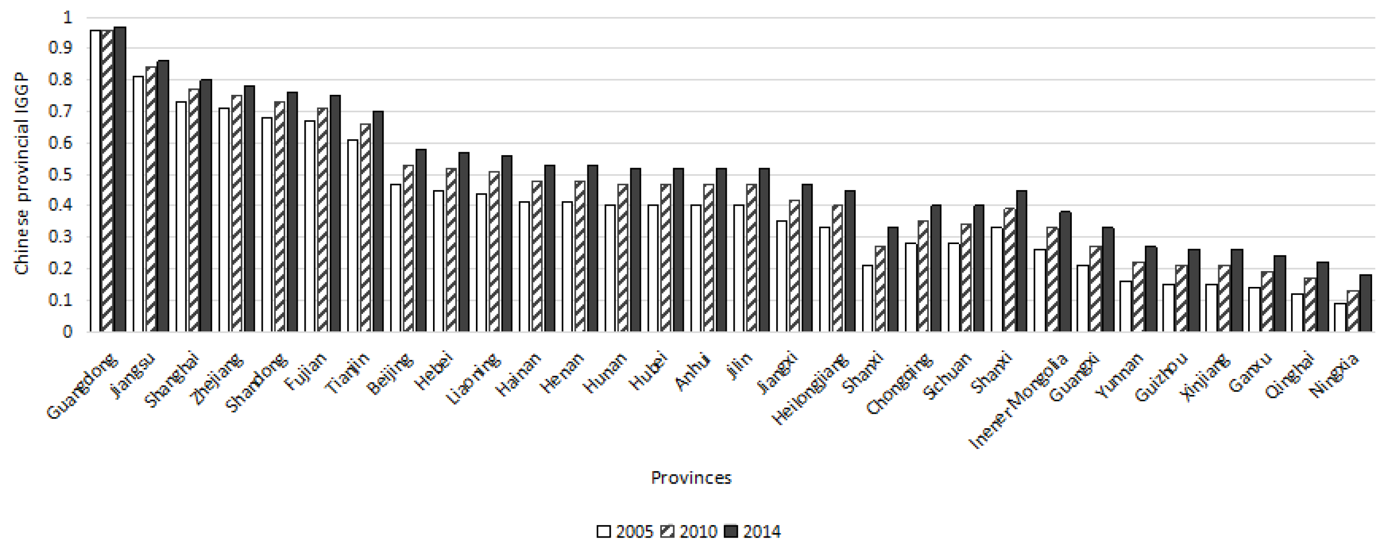
Table A1 reports the results of SFA using the Frontier 4.1 software (CEPA, Brisbane, Australia). It can be seen from the estimation results that at a 1% confidence level, the t value of γ indicates that the null hypothesis is rejected and the alternative hypothesis of inefficiency in China’s IGGP is accepted. Though several variables do not pass the t test, the model is still valid. Figure 1 and Figure 2 report the results of China’s provincial IGGP from 2000 to 2014. Overall, the IGGP is low but shows a trend of continuous improvement. From the perspective of regional level, the IGGP in eastern China was much higher than the central region, whereas the western region exhibited the lowest level. In brief, the IGGP decreased from eastern China to central and western China. Regarding to provincial level, on average, province like Guangdong, Jiangsu, Shanghai, Zhejiang and Shandong has a relative higher IGGP. The common feature of these provinces is that they are located in the economically developed southeast coastal China. Generally, this area attracts the majority of foreign investment and advancing technology. Economy in this region is prone to foreign trading, service industries, and light industries. On the other hand, the values for Ningxia, Qinghai, Gansu, Xinjiang and Guizhou were relatively lower, which are mainly located in western China, the economic development in these regions is still lagging behind with labor-intensive and resource-intensive industries, and environmental protection is inadequate. In all, the spatial distribution characteristics of IGGP in China can be described as ‘‘high in the east and low in the west”.
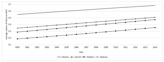
Figure 1.
The average values of Chinese industrial green growth performance (IGGP) during 2000–2014.
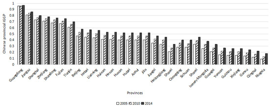
Figure 2.
The IGGP of Chinese provinces in 2005, 2010 and 2014.
3.2. Estimation Results of the Spatial Autocorrelation
We use the software OpenGeoDa to calculate the global Moran’s I index of IGGP from 2000 to 2014 in China to observe the overall spatial agglomeration or dispersion. It can be seen from Table 2, the global Moran’s I index of IGGP in 30 provinces and regions in China ranges from 0.468 to 0.485 and passed the significance test at 1% level, which indicate that positive spatial autocorrelations existed in terms of China’s IGGP. And the geographic distribution of IGGP tends to cluster together but not completely random, which means that province with a higher (or lower) efficiency value often has neighboring provinces with a higher (or lower) efficiency value.
Table 2.
Global Moran’s I Index of regional industrial green growth performance (IGGP) and its significance.
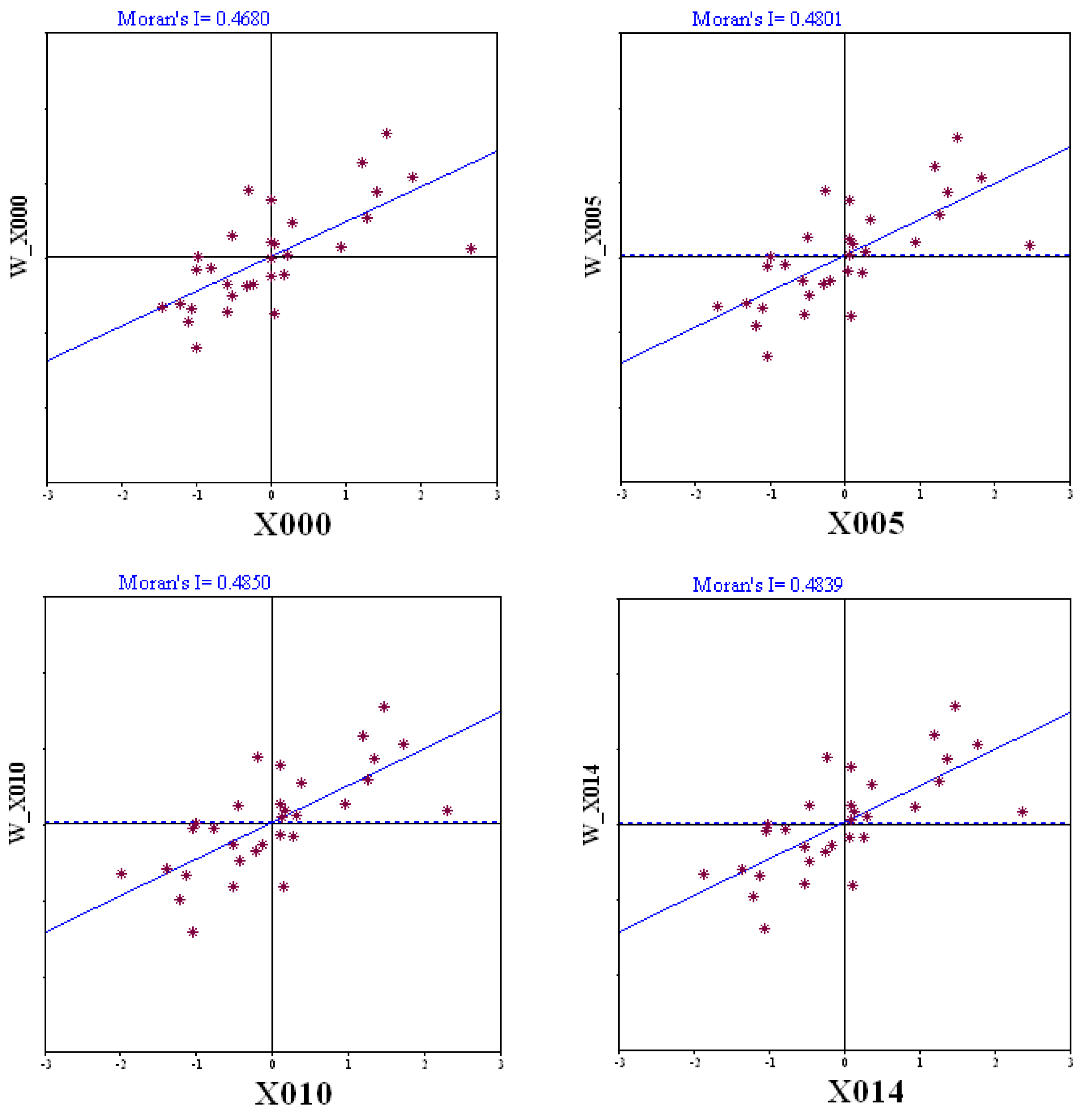
Given the limitation of the global Moran’s I test (it can only be used to explain the overall average correlation. The effects will offset each other when there are positive spatial autocorrelations in some provinces and negative spatial autocorrelation in other provinces, thus the Moran’s I index may tend to be zero which show non-spatial autocorrelation), we further draw Moran’s I scatter plots of IGGP in 2000, 2005, 2010 and 2014 to test the spatial dependence. It can be seen from Figure 3, 26 provinces (86.67%) in 2000, 26 provinces (86.67%) in 2005, 25 provinces (83.33%) in 2010, and 25 provinces (83.33%) in 2014 are HH and LL clustering, showing a positive spatial autocorrelation. From 2000 to 2014, the number of provinces in LL clustering decreased by 2 and the HH clustering increased by 1, while the number of the LH and HL clustering increased by 0 and 1, respectively. The results imply that the degree of spatial clustering of IGGP seemed to be varying during the sample period.
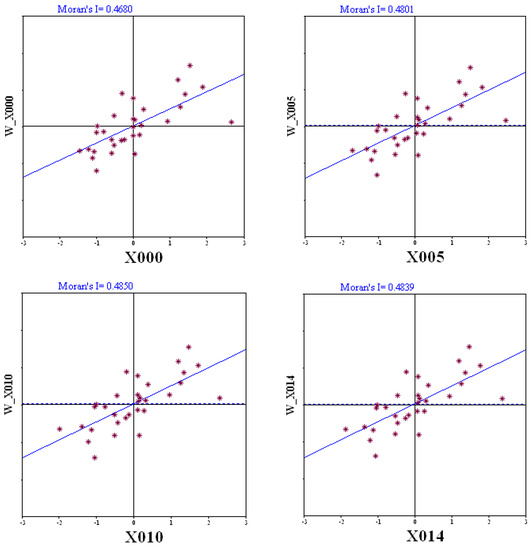
Figure 3.
Moran’s I scatter plots of China’s IGGP through time.
3.3. Spatial Econometric Analysis
Above results of the Moran’s I indicate that China’s IGGP has a significant spatial dependence. However, Moran’s I analysis itself does not clarify how different ER affect IGGP. Given the spatial dependence of IGGP, the non-spatial panel model may result in an estimated bias. Thus, the spatial panel econometric model is preferable. To decide which spatial econometric model is more appropriate, both the fixed and random effects of SDM are estimated. Since the sign of the variables in the fixed effects and the random effects models are identical, and the research objects of this study are provincial IGGP in China, the fixed effect model is preferable.
Table 3 presents the results of SLM, SEM and SDM. In terms of the Log-L of and Adj-R2 value, the fitness of the SDM model is better than that of SLM and SEM. Moreover, the spatial autoregressive coefficients ρ (in SEM) or δ (in SLM) are significantly positive. This implies that there is obvious spatial dependence in IGGP, meaning that the IGGP of one province is influenced by both the local economic activity and the neighboring provinces because of spatial spillovers.
Table 3.
Spatial econometric estimation results.
Since the coefficients of the SDM model cannot directly describe the marginal effects of variables on IGGP [27]. Table 4 displays the direct, indirect and total effects of the three different ERs and various control variables. The direct effects of the explanatory variables are different from their coefficient estimates because of the feedback effects which reflect the impact passing through surrounding regions and at last back to the regions themselves. Feedback effects equals to the difference between the elasticity coefficients and direct effects, which result from the coefficients of the spatially lagged dependent variables and the coefficients of the spatially lagged values of the explanatory variables themselves.
Table 4.
The direct effects, indirect effects, and total effects of the spatial Durbin model.
The spillover effect of AER is significantly negative, which amounts to −0.9278, larger than its direct effect (−0.2224). This indicates that an increase of AER in surrounding provinces will decrease the IGGP in the local province. In recent years, under the encouragement of the “political promotion” mechanism based on local GDP level, local governments have taken advantage of local protectionism and market segmentation to prevent various production factors from free exchange. This is the obstacle for the introduction of advanced production technologies in neighboring regions and restrains the positive spillover effect on IGGP. The reason for AER without achieving a positive direct effect on the region is that local governments are under pressure from GDP growth. Although the entry of polluting industries will destroy the ecological environment of the region, these industries can become the engine and important source of taxation of regional GDP growth. If strict AER is implemented, these industries will inevitably migrate to other regions with lower regulatory standards, which is not conducive to GDP growth and tax revenue in the region, and is not conducive to the promotion of local officials. Under the dual pressure of performance appraisal and economic development, the increasingly fierce AER competition has caused local government environmental policies to fail.
In comparison with the results of Zhao et al. [20,21], the common feature is that MER has a positive impact (that is, total effect), and the difference is that studies [20,21] failed to separate the indirect from direct effects, while in our study, we found that the spillover effect of MER amounts to 1.4316 and outperforms the negative direct effect (−0.2499) of MER, implying a positive and significant total effect (1.1817). This indicates that when a region increases the intensity of MER, it will have a large positive spillover effect on neighboring regions, while an adverse effect on itself. When the intensity of MER in a region increases, as for itself, the increase in sewage charges will stimulate enterprises to increase investment in technical innovation and can have a positive effect on efficiency; however, some enterprises in the local region have been forced to move out due to excessive sewage charges, which has a negative influence on efficiency. At present, the negative influence is even greater. For the neighboring regions, while receiving some enterprises, they will also absorb some advanced technologies to promote the increase of industrial green growth efficiency. Besides, MER has greatly promoted IGGP in general. However, the difference between direct and indirect effects indicates that central and local governments will adopt different attitudes toward MER. The main consideration of local governments is whether they can bring direct benefits to the local region. Therefore, local governments are unlikely to increase the intensity of MER. The central government, on the other hand, considers the overall situation and focuses on the total and indirect effects of MER, and will support the strengthening of MER.
The direct and indirect effects of VER are both significantly positive, reflecting that an increase in intensity of VER in a region has a positive effect on IGGP not only in the local region, but also in neighboring regions. However, the regression coefficients are very small, which amounts to 0.0001 and 0.0002, respectively. It illustrates that the awareness of environmental protection participation of the public in China is relatively weak, and most of the citizens will be petitioned after they have been affected and lack of initiative. This further indicates that the government’s environmental information disclosure is not transparent, the channels for public participation in environmental regulation are not smooth, and environmental education for the public is not in place. This result is in line with that of Ren et al. [22], indicating that with the unsound laws and regulations in western region, the efficiency of government handling environmental letters and visits is low, and few enterprises with environment labels, not to mention to the disclosure of environment events, thus, the impact of VER on eco-efficiency in western areas is weak.
With regard to the controlled variables, the direct and total effects of FDI are significantly positive, which indicates that FDI is crucial in improving China’s industrial development because it can alleviate environmental pollution through the transfer of clean technologies, at the same time, FDI helps to improve industrial productivity through the technology diffusion. However, the spillover effect of FDI is significantly negative, indicating that some FDI are prone to transfer energy and pollution-intensive industries from the advanced areas to the relatively backward areas with weaker ERs to save production costs. Meanwhile, since the GDP level, human capital, financial development level and degree of openness in different regions of China are heterogeneous, which results in different knowledge and technical absorption capacity. Finally, market competition enables areas with comparatively low economic capacity to lower their environment standard in order to attract more FDI, leading to a situation of “race to the bottom”.
Regarding to ESC, all the direct, indirect and total effects are significantly negative, which indicates that a higher is the ratio of coal consumption to total energy consumption will lead to a more adverse effect on IGGP. Just as the previous study [29] found that the ESC in most industrial departments have much space for enrichment. Thus, the amelioration of ECS aims to increase non-fossil energy use and cut fossil energy use.
The direct and total effects of TL are significantly positive, while the indirect effect is negative. The results show that TL is the fundamental driving force of China’s IGGP. Technological innovation can optimize the production process through increasing the utilization of factors and promote the conservation and recycling of natural resources, resulting in lower natural resource consumption under a given output, and then improve IGGP. The negative spillover effect may be due to a higher TL in the region attracting innovative talents in the surrounding area, resulting in a lower technological innovation level in the surrounding area.
4. Conclusions and Policy Implications
This paper estimated a SFA model to calculate China’s provincial IGGP from 2000 to 2014, which indicates that the IGGP in most regions of China shows a trend of continuous improvement and the distribution IGGP in China can be described as ‘‘high in the east and low in the west”. On this basis, the SDM model is applied to analyze the influencing mechanism of ER on IGGP from three dimensions of administrative, market, and public participation. The empirical results show that a significant spatial autocorrelation is existed in China’s IGGP during the sample period. The direct and indirect effects of AER are significantly negative; the direct effect of MER is significantly negative, but the indirect effect are is significantly positive; the direct and indirect effects of VER are both significantly positive, but the coefficients are small. The results stress the significance of considering spatial dependence to legitimately use various ER tools to promote IGGP. According to the conclusions, we propose the following relevant policy suggestions:
- Rationally use AER instruments to promote the process of regional integration. Because of the different economic patterns in different regions, the applicability of policies is not identical. Therefore, in formulating specific AER policies, “one size fits all” should be avoided. Local governments should formulate corresponding AER based on the different characteristics of industries in each region. On this basis, multi-target performance appraisal mechanisms should be introduced so that local governments no longer focus on economic development but ignore the environment. We must also work hard to promote the regional cooperation, achieve the sharing of benefits, eliminate various trade barriers and market barriers, and remove obstacles to promote the flow of funds, talent, and technology among different regions. In addition, it is necessary to increase supervision over administrative controls to ensure that environmental protection investment is used compliantly and efficiently and prevent rent-seeking behaviors.
- Complete MER tools and establish environmental compensation mechanisms. It is crucial to promote the process of replacing the green taxes sewage charges with the environmental taxes, and strength the intensity of MER, so as to force the elimination of backward production capacity. Meanwhile, it should also actively learn from the developed countries and continuously enrich MER tools in accordance with China’s national conditions. In view of the different attitudes between the central government and local governments toward MER, in order to prevent the emergence of environmental competition among regions, appropriate environmental compensation mechanisms should be established. At the same time, policy-makers may as well make clear provisions on compensation standards and actively coordinate regional environmental compensation.
- Strengthen government supervision and exert the role of VER in maximize extent. Related departments should encourage and guide public to take part in environmental protection. First of all, it is necessary to strengthen advocating to improve the public awareness of environmental protection. Then, relevant departments should complete legislation as soon as possible to provide legal protection for citizens to exercise the right to know and supervise. Furthermore, government should publish relevant environmental construction projects through the media in time, and fully listen to public opinions through seminars, hearings, questionnaires.
- Additionally, FDI has a significant role in promoting China’s IGGP. China’s government should further improve the policies of FDI inflow. For example, strictly restricting the entry of low-tech foreign-funded companies, positively encouraging the introduction of high-tech foreign-funded companies and related advanced technologies. Moreover, given the imbalance in development of various regions in China, the underdeveloped regions should think highly of improving the quality of foreign investment. In addition, the underdeveloped areas should strengthen infrastructure construction and enhance the human capital level to reduce the disadvantageous technology spillover effects of FDI on the quality of environment.
- Furthermore, it is vital to improve the ratio of non-fossil energy to the overall energy consumption. Given the difference of energy endowments in various regions, ECS is diverse. The government should positively push forward the market-oriented reform of energy pricing mechanism according to the differentiated features of ESC of industrial sectors in various areas.
- Finally, the conclusions also indicate that higher TL is beneficial to IGGP and social environmental protection to a certain extent, IGGP could be stimulated if industrial sector input in technology. According to the results, we suggest that under strengthening technology introduction and independent innovation, we must pay special attention to technology absorption and application promotion related to energy-saving and environmental protection, improve government related investment, guide and encourage private capital to enter emission reduction, transform and upgrade traditional industries while actively develop modern manufacturing technologies, and promote the extension of manufacturing and its products to the high end of the technology chain.
Author Contributions
All authors contributed equally to this work. M.L. wrote the initial manuscript draft; and X.W. performed several significant revisions.
Funding
This research received no external funding.
Conflicts of Interest
The authors declare no conflict of interest.
Appendix A
Table A1.
The results of estimation of trans-log stochastic production function.
Table A1.
The results of estimation of trans-log stochastic production function.
| Variables | Coefficient | T-Ratio | Variables | Coefficient | T-Ratio |
|---|---|---|---|---|---|
| 3.294 *** | 3.047 | 1.061 *** | 3.769 | ||
| 0.388 *** | 8.722 | 0.277 ** | 2.130 | ||
| 0.003 | 1.278 | −0.107 *** | -2.926 | ||
| 0.624 ** | 2.165 | 0.034 | 0.166 | ||
| 0.332 ** | 2.245 | −0.084 | −0.409 | ||
| −2.128 *** | −3.291 | −0.142 | −0.882 | ||
| 1.573 *** | 2.794 | 0.217 ** | 1.972 | ||
| 0.017 *** | −2.612 | −1.192 ** | −2.379 | ||
| 0.006 | 0.778 | σ² | 0.299 *** | 10.327 | |
| −0.095 *** | −5.636 | γ | 0.952 *** | 142.714 | |
| 0.069 *** | 4.948 | mu | 1.068 *** | 9.372 | |
| 0.012 | 0.202 | eta | −0.029 *** | −7.504 | |
| -0.034 | −0.588 | LR | 541.901 | ||
Note: ***, ** indicate the significance levels are 1%, 5% respectively.
References
- NBSC (National Bureau of Statistics of China). China Statistical Yearbook 2017; China Statistics Press: Beijing, China, 2017.
- OECD. Towards Green Growth: Monitoring Progress; OECD: Paris, Frnace, 2011. [Google Scholar]
- Gunningham, N.; Grabosky, P.N.; Sinclair, D. Smart Regulation: Designing Environmental Policy; Socio-Legal Studies: Oxford, UK, 1998. [Google Scholar]
- Huang, J.H.; Yang, X.G.; Cheng, G.; Wang, S.Y. A comprehensive eco-efficiency model and dynamics of regional eco-efficiency in China. J. Clean. Prod. 2014, 67, 228. [Google Scholar] [CrossRef]
- Zhang, N.; Kong, F.B.; Yu, Y.N. Measuring ecological total-factor energy efficiency incorporating regional heterogeneities in China. Ecol. Indic. 2015, 51, 165. [Google Scholar] [CrossRef]
- CIIGBC (Confederation of Indian Industry-Sohrabji Godrej Green Business Centre). Green Company Rating System. 2012. Available online: http://www.greenbusinesscentre.com/ CII-Publication/greenco.html (accessed on 5 July 2016).
- Li, X.X.; Pan, J.C. China Green Development Index Report 2011; Springer-Verlag: Heidelberg, Germany, 2013. [Google Scholar]
- Shi, G.M.; Bi, J.; Wang, J.N. Chinese regional industrial energy efficiency evaluation based on a DEA model of fixing non-energy inputs. Energy Policy 2010, 38, 6172. [Google Scholar] [CrossRef]
- Zhang, J.X.; Liu, Y.M.; Chang, Y.; Zhang, L.X. Industrial eco-efficiency in China: A provincial quantification using three-stage data envelopment analysis. J. Clean. Prod. 2017, 143, 238. [Google Scholar] [CrossRef]
- Wu, J.; Zhu, Q.; Chu, J.; Liang, L. Two-stage network structures with undesirable intermediate outputs reused: A DEA based approach. Comput. Econ. 2015, 46, 455. [Google Scholar] [CrossRef]
- Aigner, D.; Lovell, C.A.K.; Schmit, P. Formulation and estimation of stochastic frontier production function models. J. Econom. 1977, 6, 21. [Google Scholar] [CrossRef]
- Lin, B.Q.; Yang, L.S. The potential estimation and factor analysis of China’s energy conservation on thermal power industry. Energy Policy 2013, 62, 354. [Google Scholar] [CrossRef]
- Ouyang, X.L.; Sun, C.W. Energy savings potential in China’s industrial sector: From the perspectives of factor price distortion and allocative inefficiency. Energy Econ. 2015, 48, 117. [Google Scholar] [CrossRef]
- Gray, W.B. The cost of regulation: OSHA, EPA and the productivity slowdown. Am. Econ. Rev. 1987, 77, 998. [Google Scholar]
- Jorgenson, D.W.; Wilcoxen, P.J. Environmental Regulation and U.S. Economic Growth. Rand J. Econ. 1990, 21, 314. [Google Scholar] [CrossRef]
- Wu, M.Q.; Zhou, S.M.; Chen, J.C. Can environmental regulation and economic growth be a win-win situation? Based on the empirical research of China’s “two control areas”. Contemp. Econ. Sci. 2016, 38, 44. [Google Scholar]
- Lu, K.J.; Cheng, Y.; Fan, B.J. The Impact of Environmental Regulation on Green Total Factor Productivity of Chinese Manufacturing Industry. Ecol. Econ. 2017, 33, 49. [Google Scholar]
- Wang, J.; Liu, B. Environmental Regulation and Corporate Total Factor Productivity: Empirical Analysis Based on Chinese Industrial Enterprise Data. China Ind. Econ. 2014, 3, 44. [Google Scholar]
- Yan, Y.G.; Chang, R. Environmental Regulation and Industrial Total Factor Productivity: Empirical Study Based on Dynamic Panel Data of 280 Prefecture-level Cities. Econ. Issues 2016, 11, 18. [Google Scholar]
- Zhao, X.; Yin, H.; Zhao, Y. Impact of environmental regulations on the efficiency and CO2 emissions of power plants in China. Appl. Energy 2015, 149, 238. [Google Scholar] [CrossRef]
- Zhao, X.; Zhao, Y.; Zeng, S.; Zhang, S. Corporate behavior and competitiveness: Impact of environmental regulation on Chinese firms. J. Clean. Prod. 2015, 86, 311. [Google Scholar] [CrossRef]
- Ren, S.; Li, X.; Yuan, B.; Li, D.; Chen, X. The effects of three types of environmental regulation on eco-efficiency: A cross-region analysis in China. J. Clean. Prod. 2018, 173, 245. [Google Scholar] [CrossRef]
- Tobler, W. A computer movie simulating urban growth in the Detroit region. Econ. Geogr. 1970, 46, 234. [Google Scholar] [CrossRef]
- Kumbhakar, S.C. Estimation and decomposition of productivity change when production is not efficient: A panel data approach. Econom. Rev. 2000, 19, 425. [Google Scholar] [CrossRef]
- Shao, B.B.M.; Lin, W.T. Assessing output performance of information technology service industries: Productivity, innovation and catch-up. Int. J. Prod. Econ. 2016, 172, 43–53. [Google Scholar] [CrossRef]
- Shao, S.; Luan, R.R.; Yang, Z.B.; Li, C.Y. Does directed technological change get greener: Empirical evidence from Shanghai’s industrial green development transformation. Ecol. Indic. 2016, 69, 758. [Google Scholar] [CrossRef]
- Lesage, J.P.; Pace, R.K. Introduction to Spatial Econometrics; Press/Taylor & Francis: Boca Raton, FL, USA, 2009; p. 20. [Google Scholar]
- National Bureau of Statistics of China. China Energy Statistical Yearbook; China Statistic Press: Beijing, China, 2012.
- Yang, Z.B.; Shao, S.; Yang, L.L.; Miao, Z. Improvement pathway of energy consumption structure in China’s industrial sector: From the perspective of directed technical change. Energy Econ. 2018, 72, 166. [Google Scholar] [CrossRef]
© 2019 by the authors. Licensee MDPI, Basel, Switzerland. This article is an open access article distributed under the terms and conditions of the Creative Commons Attribution (CC BY) license (http://creativecommons.org/licenses/by/4.0/).