An Analytical Solution of the Pseudosteady State Productivity Index for the Fracture Geometry Optimization of Fractured Wells


Abstract
1. Introduction
2. Analytical Solution of the Pseudosteady State Productivity Index
2.1. The Model
- (1)
- When :where is the proppant number and is the dimensionless fracture conductivity. The fitting function is given in Equation (A7) and the analytical expression of the shape factor is given in Equation (A9).
- (2)
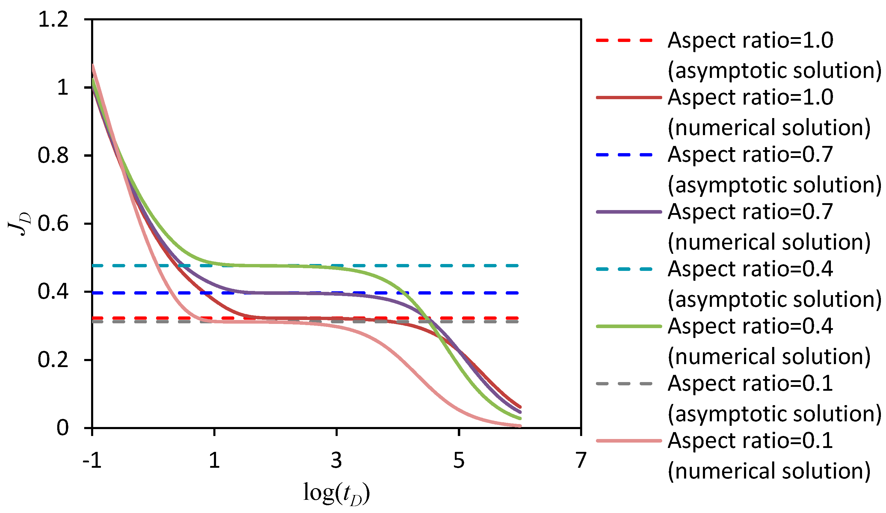
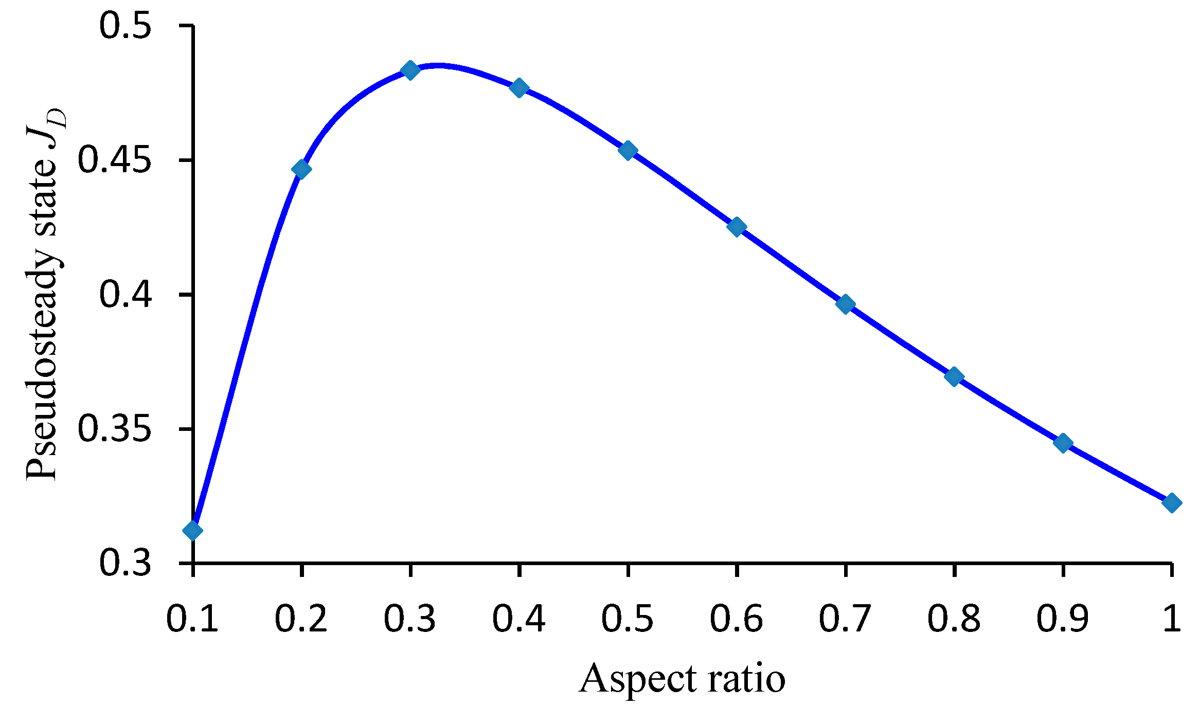
- When :where is the aspect ratio of the rectangular drainage area defined in Appendix A.
2.2. Verification
3. Fracture Geometry Optimization
3.1. Comparison with the Unified Fracture Design Method
- (1)
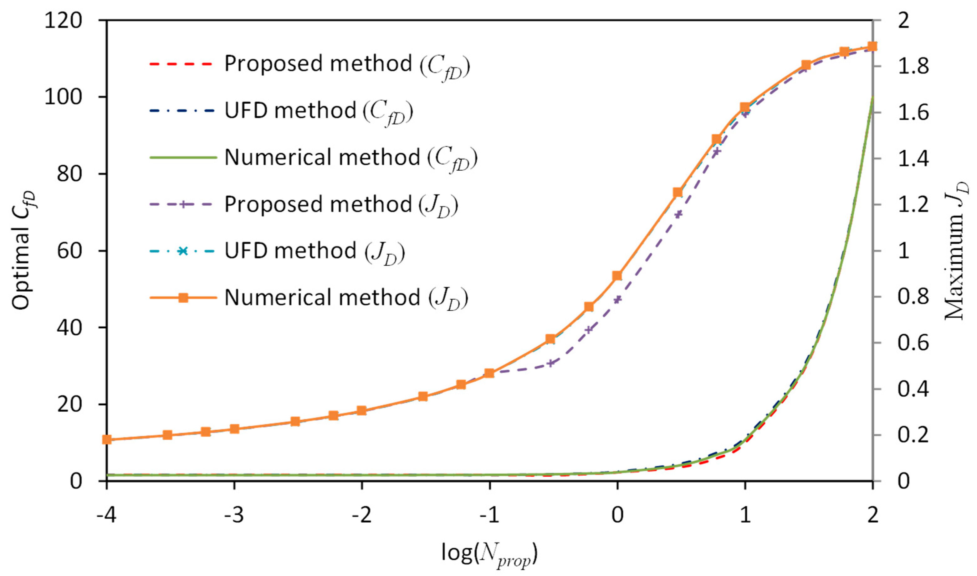
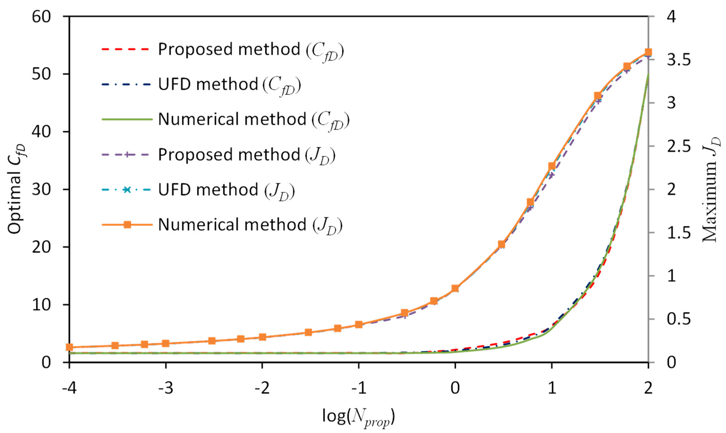
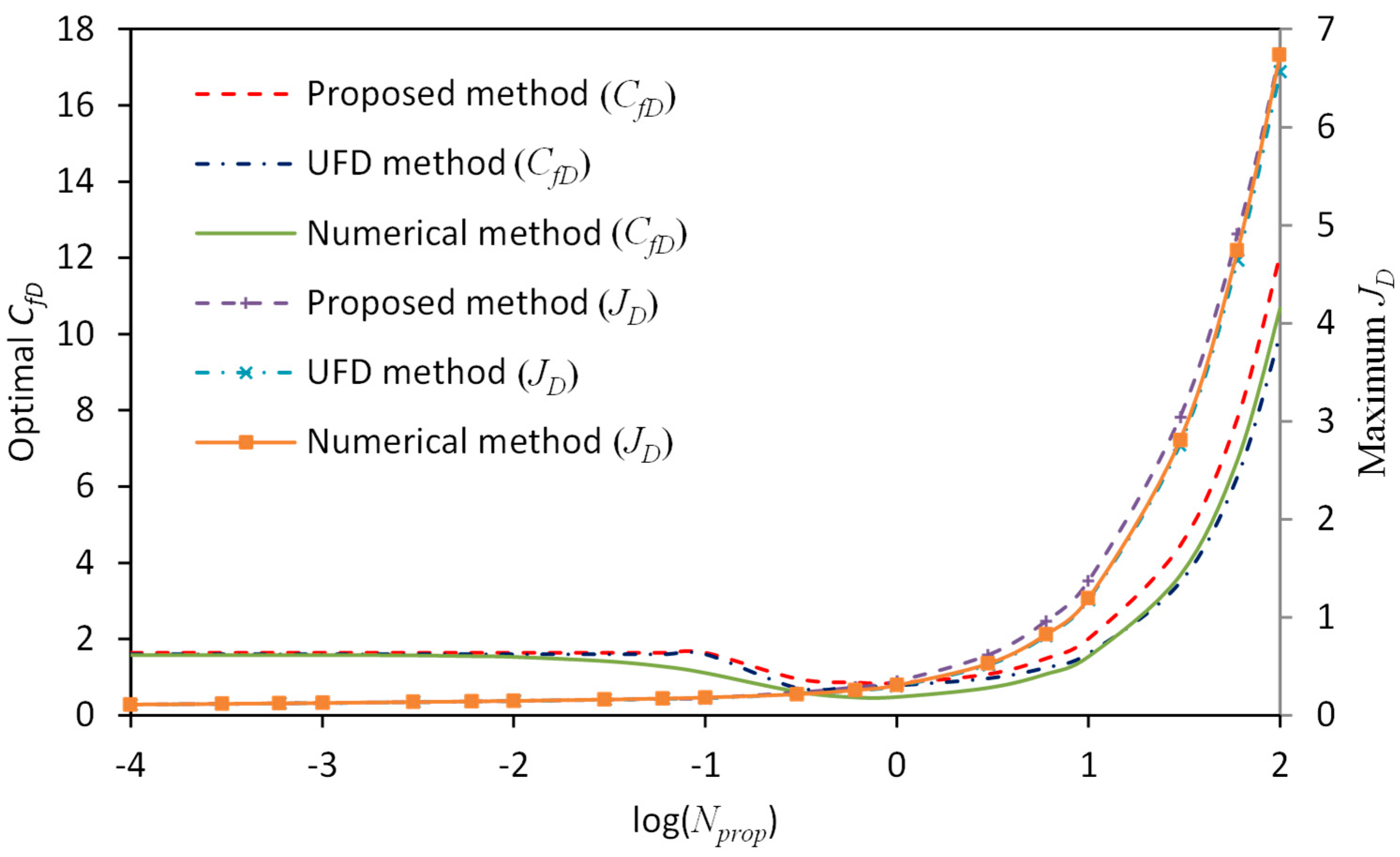
- When is within the intermediate range, for example, 0.1–1.0, the UFD method suffers from interpolation error if the value of is not given in Table A1 or Table A2. However, the proposed method is applicable for arbitrary aspect ratios and the results agree well with true values obtained by the numerical method.
- (2)
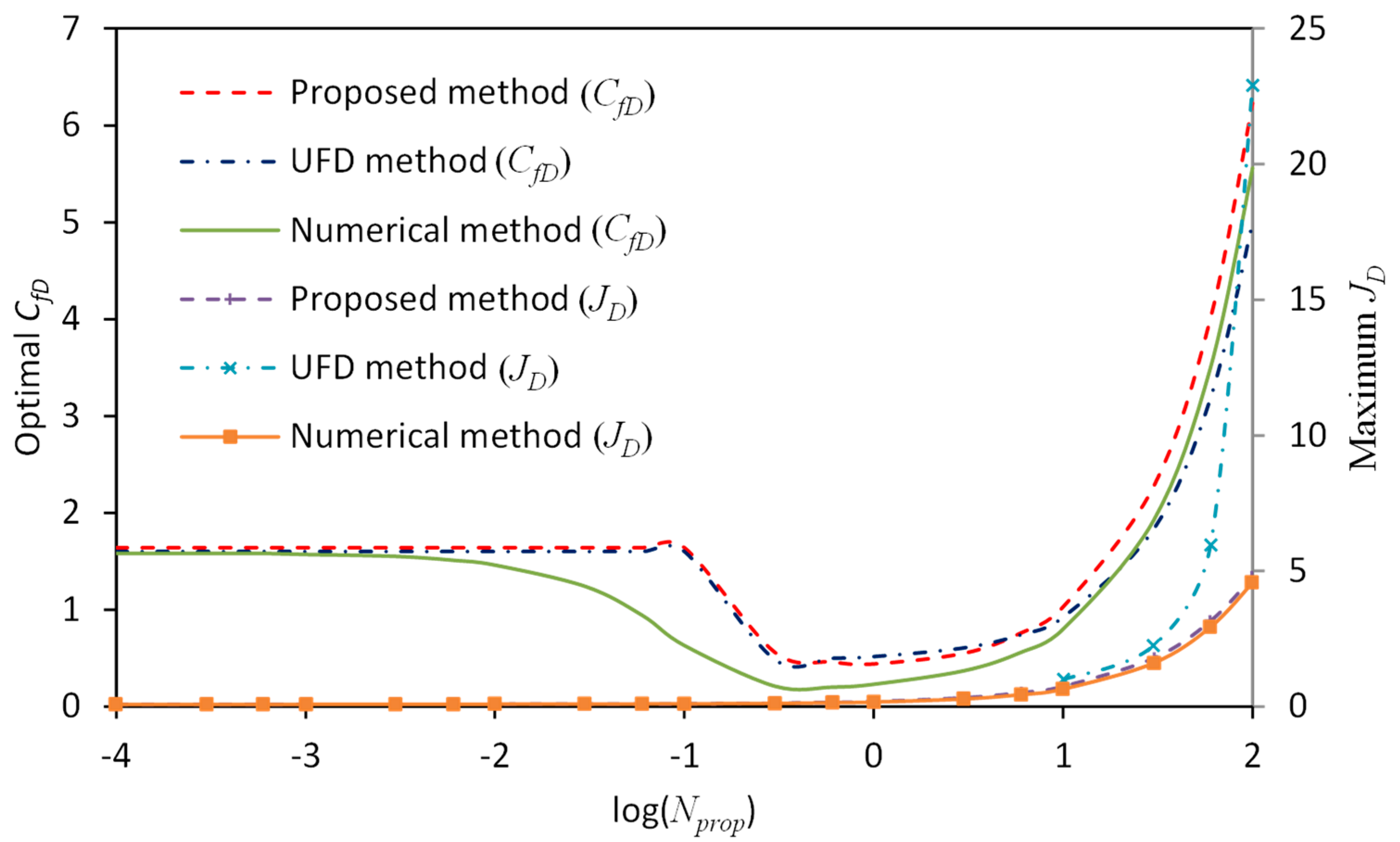
- For less than 0.1 or larger than 1.0, the UFD method suffers from extrapolation error. In particular, deviates seriously from true values given by the numerical method.
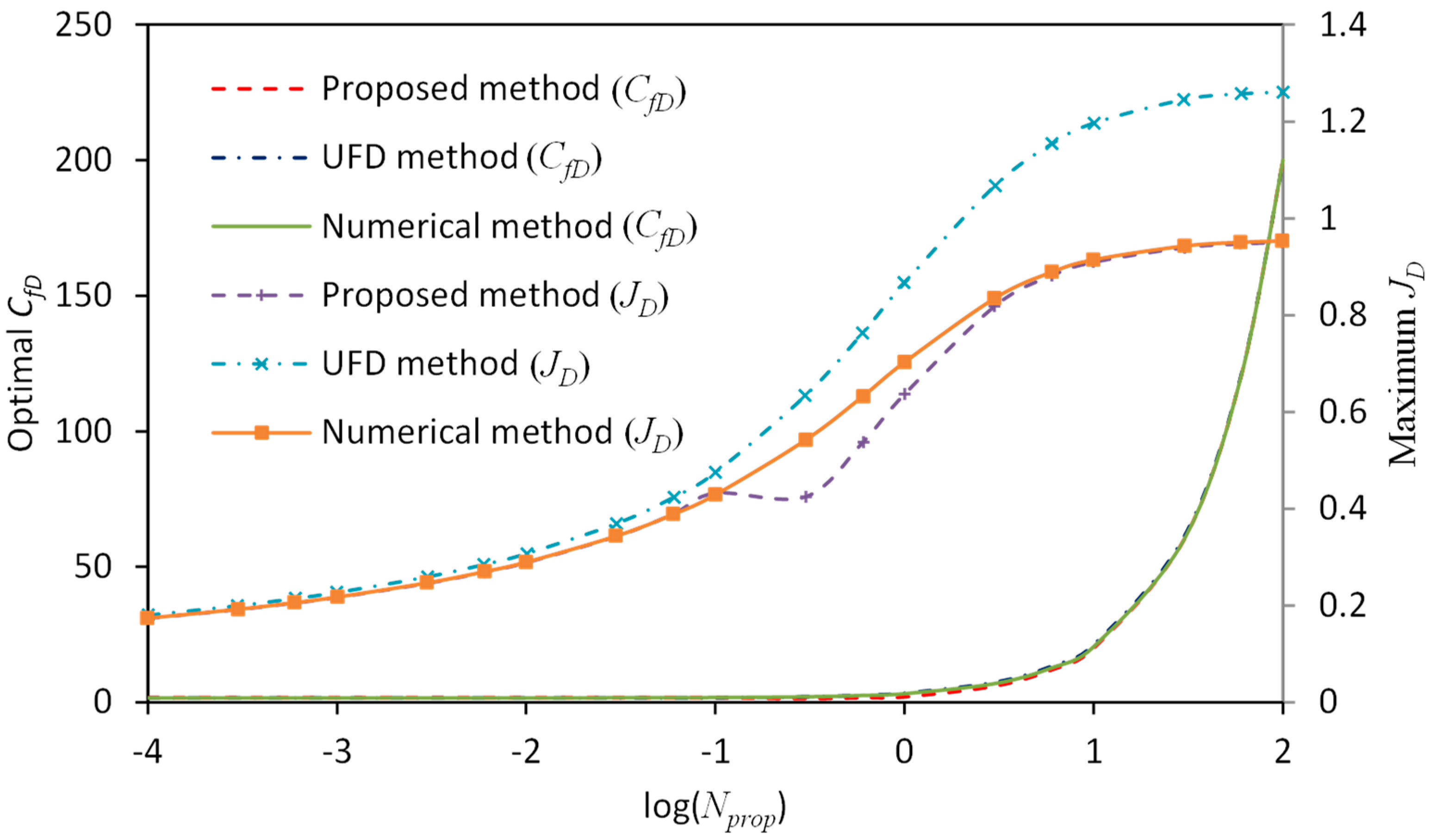
- (3)
- For less than 0.1, values obtained by the proposed method deviate from the true values within the transition region. On the other hand, for larger than 1.0, error occurs for obtained by the proposed method within the transition region. The reason is probably that when the aspect ratio of the drainage area becomes too small or too large, flow in the reservoir-fracture system deviates from the trilinear-flow model and new models should be applied together with the current model in the future study.
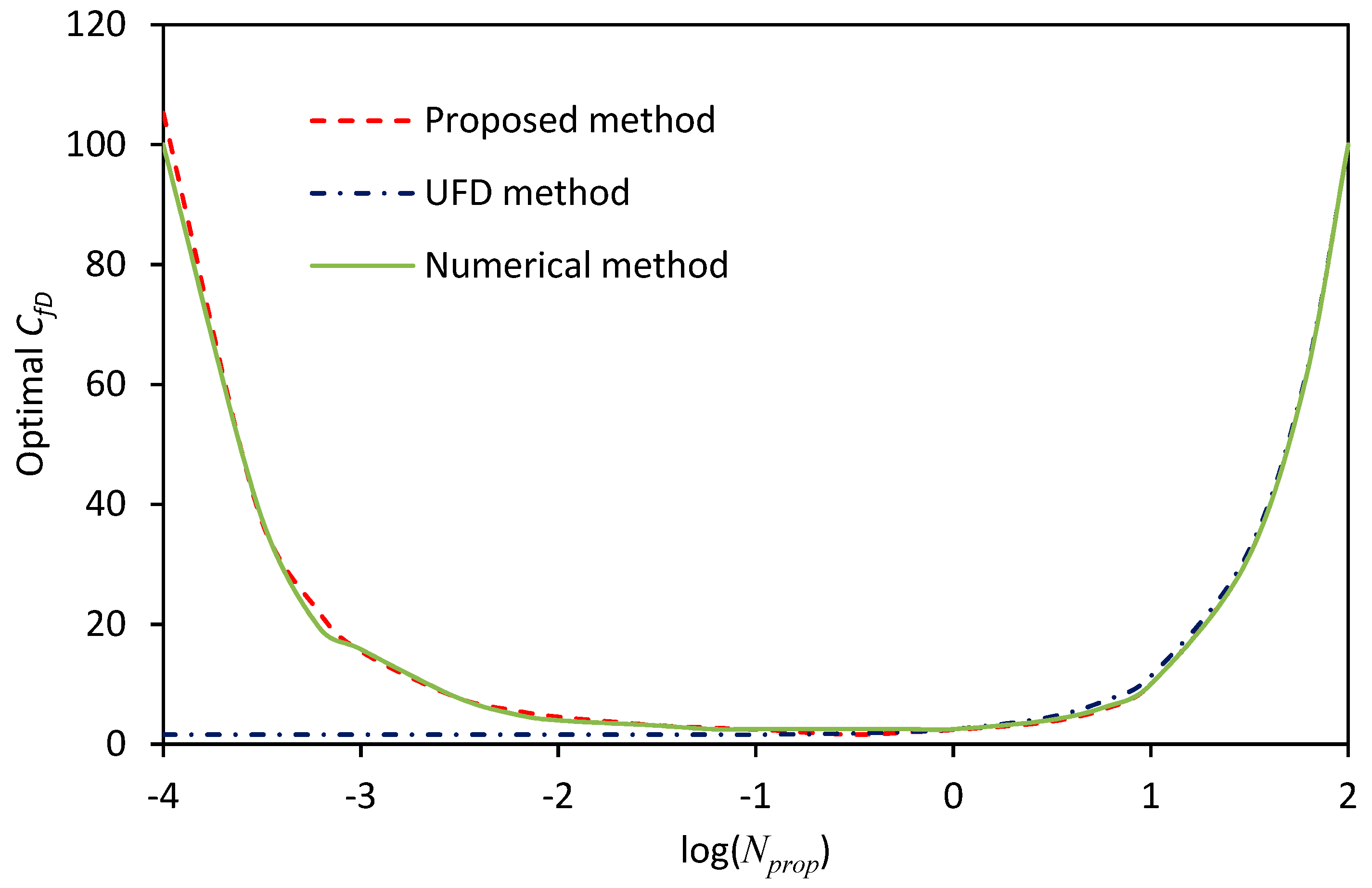
3.2. Considering the Radial Flow Skin Factor
4. Conclusions
- (1)
- The proposed analytical formulas provide solutions of the dimensionless productivity index for any dimensionless fracture conductivity value and proppant number, whereas the UFD method only provides fitting solutions of the maximum productivity index corresponding to the optimal fracture conductivity.
- (2)
- Using the proposed analytical solution of the pseudosteady state productivity index, optimized fracture geometry dimensions can be obtained for arbitrary aspect ratios of rectangular drainage areas, whereas the UFD method suffers from interpolation or extrapolation error if the value of the aspect ratio is not given in related tables.
- (3)
- By explicitly considering the skin factor caused by the radial flow choking of fractured horizontal wells in dimensionless fracture conductivity optimization, the result is more accurate than that obtained by the UFD method.
Author Contributions
Funding
Conflicts of Interest
Appendix A. Fitting Solution for Proppant Numbers Less Than 0.1

Appendix B. Asymptotic Solution for Proppant Numbers Greater Than 0.1
Appendix C. Unified Fracture Design (UFD) Method


| 0.1 | 0.2 | 0.25 | 0.3 | 0.4 | 0.5 | 0.6 | 0.7 | 0.8 | 0.9 | 1.0 | |
|---|---|---|---|---|---|---|---|---|---|---|---|
| 0.025 | 2.36 | 5.38 | 9.00 | 16.17 | 21.84 | 25.80 | 28.36 | 29.89 | 30.66 | 30.88 |
| 1 | 0.7 | 0.5 | 0.25 | 0.2 | 0.1 | |
|---|---|---|---|---|---|---|
| a | 17.2 | 17.4 | 21.4 | 38.3 | 35 | 30.6 |
| b | 54.5 | 55.5 | 54.3 | 46 | 59 | 89.6 |
| c | 52.5 | 53.3 | 56.3 | 71.1 | 70 | 70.2 |
| d | 16.9 | 16.9 | 16.9 | 15.84 | 16.3 | 17.8 |
| a’ | 10 | |||||
| b’ | 36 | |||||
| c’ | 33 | |||||
References
- Gringarten, A.C.; Ramey, H.J. The Use of Source and Green’s Functions in Solving Unsteady-Flow Problems in Reservoirs. Soc. Pet. Eng. J. 1973, 13, 285–296. [Google Scholar] [CrossRef]
- Gringarten, A.C.; Ramey, H.J.; Raghavan, R. Unsteady-State Pressure Distributions Created by a Well with a Single Infinite-Conductivity Vertical Fracture. Soc. Pet. Eng. J. 1974, 14, 347–360. [Google Scholar] [CrossRef]
- Guo, G.; Evans, R.D. Pressure-Transient Behavior and Inflow Performance of Horizontal Wells Intersecting Discrete Fractures. In Proceedings of the SPE Annual Technical Conference and Exhibition, Houston, TX, USA, 3–6 October 1993. [Google Scholar]
- Horne, R.N.; Temeng, K.O. Relative Productivities and Pressure Transient Modeling of Horizontal Wells with Multiple Fractures. In Proceedings of the SPE Middle East Oil Show, Manama, Bahrain, 11–14 March 1995. [Google Scholar]
- Lei, Z.; Cheng, S.; Li, X.; Xiao, H. A new method for prediction of productivity of fractured horizontal wells based on non-steady flow. J. Hydrodyn. 2007, 19, 494–500. [Google Scholar] [CrossRef]
- Zeng, F.; Long, C.; Guo, J. A novel unsteady model of predicting the productivity of multi-fractured horizontal wells. Int. J. Heat Technol. 2015, 33, 117–124. [Google Scholar] [CrossRef]
- Hu, J.; Zhang, C.; Rui, Z.; Yu, Y.; Chen, Z. Fractured horizontal well productivity prediction in tight oil reservoirs. J. Pet. Sci. Eng. 2017, 151, 159–168. [Google Scholar] [CrossRef]
- Cinco, H.L.; Samaniego, F.V.; Dominguez, N.A. Transient Pressure Behavior for a Well with a Finite-Conductivity Vertical Fracture. Soc. Pet. Eng. J. 1978, 18, 253–264. [Google Scholar] [CrossRef]
- Kruysdijk, C.P. Semianalytical Modeling of Pressure Transients in Fractured Reservoirs. In Proceedings of the SPE Annual Technical Conference and Exhibition, Houston, TX, USA, 2–5 October 1988. [Google Scholar]
- Yao, S.; Zeng, F.; Liu, H.; Zhao, G. A semi-analytical model for multi-stage fractured horizontal wells. J. Hydrol. 2013, 507, 201–212. [Google Scholar] [CrossRef]
- Zhang, F.; Yang, D. Determination of Fracture Conductivity in Tight Formations with Non-Darcy Flow Behavior. Soc. Pet. Eng. J. 2014, 19, 34–44. [Google Scholar] [CrossRef]
- Chen, H.Y.; Poston, S.W.; Raghavan, R. An Application of the Product Solution Principle for Instantaneous Source and Green’s Functions. SPE Form. Eval. 1991, 6, 161–167. [Google Scholar] [CrossRef]
- Riley, M.F.; Brigham, W.E.; Horne, R.N. Analytic Solutions for Elliptical Finite-Conductivity Fractures. In Proceedings of the SPE Annual Technical Conference and Exhibition, Dallas, TX, USA, 6–9 October 1991. [Google Scholar]
- Larsen, L.; Hegre, T.M. Pressure-Transient Behavior of Horizontal Wells with Finite-Conductivity Vertical Fractures. In Proceedings of the SPE International Arctic Technology Conference, Anchorage, AK, USA, 29–31 May 1991. [Google Scholar]
- Larsen, L.; Hegre, T.M. Pressure Transient Analysis of Multifractured Horizontal Wells. In Proceedings of the SPE Annual Technical Conference and Exhibition, New Orleans, LA, USA, 25–28 September 1994. [Google Scholar]
- Wan, J.; Aziz, K. Semi-Analytical Well Model of Horizontal Wells with Multiple Hydraulic Fractures. Soc. Pet. Eng. J. 2002, 7, 437–445. [Google Scholar] [CrossRef]
- Wang, L.; Wang, X.; Zhang, H.; Hu, Y.; Li, C. A Semianalytical Solution for Multifractured Horizontal Wells in Box-Shaped Reservoirs. Math. Probl. Eng. 2014, 2014, 716390. [Google Scholar] [CrossRef]
- Zhao, Y.; Zhang, L.; Luo, J.; Zhang, B. Performance of fractured horizontal well with stimulated reservoir volume in unconventional gas reservoir. J. Hydrol. 2014, 512, 447–456. [Google Scholar] [CrossRef]
- Zhang, H.; Wang, X.; Wang, L. An Analytical Solution of Partially Penetrating Hydraulic Fractures in a Box-Shaped Reservoir. Math. Probl. Eng. 2015, 2015, 726910. [Google Scholar] [CrossRef]
- Zhao, Y.; Zhang, L.; Liu, Y.; Hu, S.; Liu, Q. Transient pressure analysis of fractured well in bi-zonal gas reservoirs. J. Hydrol. 2015, 524, 89–99. [Google Scholar] [CrossRef]
- Ozkan, E. Performance of Horizontal Wells. Ph.D. Thesis, The University of Tulsa, Tulsa, OK, USA, 1988. [Google Scholar]
- Chen, C.; Raghavan, R. A Multiply-Fractured Horizontal Well in a Rectangular Drainage Region. Soc. Pet. Eng. J. 1997, 2, 455–465. [Google Scholar] [CrossRef]
- Zerzar, A.; Bettam, Y. Interpretation of Multiple Hydraulically Fractured Horizontal Wells in Closed Systems. In Proceedings of the Canadian International Petroleum Conference, Calgary, AB, Canada, 8–10 June 2004. [Google Scholar]
- Stehfest, H. Algorithm 368: Numerical inversion of Laplace transforms. ACM 1970, 13, 47–49. [Google Scholar] [CrossRef]
- Wang, H. Performance of multiple fractured horizontal wells in shale gas reservoirs with consideration of multiple mechanisms. J. Hydrol. 2014, 510, 299–312. [Google Scholar] [CrossRef]
- Liu, Q.; Li, K.; Wang, W.; Hu, X.; Liu, H. Production Behavior of Fractured Horizontal Well in Closed Rectangular Shale Gas Reservoirs. Math. Probl. Eng. 2016, 2016, 4260148. [Google Scholar] [CrossRef]
- Zhao, Y.; Zhang, L.; Xiong, Y.; Zhou, Y.; Liu, Q.; Chen, D. Pressure response and production performance for multi-fractured horizontal wells with complex seepage mechanism in box-shaped shale gas reservoir. J. Nat. Gas Sci. Eng. 2016, 32, 66–80. [Google Scholar] [CrossRef]
- Dai, Y.; Ma, X.; Jia, A.; He, D.; Wei, Y.; Xiao, C. Pressure transient analysis of multistage fracturing horizontal wells with finite fracture conductivity in shale gas reservoirs. Environ. Earth Sci. 2016, 75, 940. [Google Scholar] [CrossRef]
- Zhang, F.; Yang, D.T. Effects of Non-Darcy Flow and Penetrating Ratio on Performance of Horizontal Wells with Multiple Fractures. In Proceedings of the SPE Unconventional Resources Conference Canada, Calgary, AB, Canada, 5–7 November 2013. [Google Scholar]
- Yang, D.; Zhang, F.; Styles, J.A.; Gao, J. Performance Evaluation of a Horizontal Well with Multiple Fractures by Use of a Slab-Source Function. Soc. Pet. Eng. J. 2015, 20, 652–662. [Google Scholar] [CrossRef]
- Lin, J.; Zhu, D. Predicting Well Performance in Complex Fracture Systems by Slab Source Method. In Proceedings of the SPE Hydraulic Fracturing Technology Conference, The Woodlands, TX, USA, 6–8 February 2012. [Google Scholar]
- Lin, J.; Zhu, D. Modeling well performance for fractured horizontal gas wells. J. Nat. Gas Sci. Eng. 2014, 18, 180–193. [Google Scholar] [CrossRef]
- Rbeawi, S.A.; Tiab, D. Effect of Penetrating Ratio on Pressure Behavior of Horizontal Wells with Multiple-Inclined Hydraulic Fractures. In Proceedings of the SPE Western Regional Meeting, Bakersfield, CA, USA, 21–23 March 2012. [Google Scholar]
- Rbeawi, S.A.; Tiab, D. Impacts of reservoir boundaries and fracture dimensions on pressure behaviors and flow regimes of hydraulically fractured formations. J. Pet. Explor. Prod. Technol. 2014, 4, 37–57. [Google Scholar] [CrossRef]
- Rbeawi, S.A.; Tiab, D. Predicting productivity index of hydraulically fractured formations. J. Pet. Sci. Eng. 2013, 112, 185–197. [Google Scholar] [CrossRef]
- Wang, J.; Li, H.; Wang, Y.; Li, Y.; Jiang, B.; Luo, W. A New Model to Predict Productivity of Multiple-Fractured Horizontal Well in Naturally Fractured Reservoirs. Math. Probl. Eng. 2015, 2015, 892594. [Google Scholar] [CrossRef]
- Amini, S. Development and Application of the Method of Distributed Volumetric Sources to the Problem of Unsteady-State Fluid Flow in Reservoirs. Ph.D. Thesis, Texas A&M University, College Station, TX, USA, 2007. [Google Scholar]
- Valko, P.P.; Amini, S. The Method of Distributed Volumetric Sources for Calculating the Transient and Pseudosteady-State Productivity of Complex Well-Fracture Configurations. In Proceedings of the SPE Hydraulic Fracturing Technology Conference, College Station, TX, USA, 29–31 January 2007. [Google Scholar]
- Amini, S.; Valko, P.P. Using Distributed Volumetric Sources to Predict Production from Multiple-Fractured Horizontal Wells Under Non-Darcy-Flow Conditions. Soc. Pet. Eng. J. 2010, 15, 105–115. [Google Scholar] [CrossRef]
- Zhu, D.; Magalhaes, F.V.; Valko, P. Predicting the Productivity of Multiple-Fractured Horizontal Gas Wells. In Proceedings of the SPE Hydraulic Fracturing Technology Conference, College Station, TX, USA, 29–31 January 2007. [Google Scholar]
- Wan, Y.; Liu, Y.; Liu, W.; Han, G.; Niu, C. A numerical approach for pressure transient analysis of a vertical well with complex fractures. Acta Mech. Sin. 2016, 32, 640–648. [Google Scholar] [CrossRef]
- Jiang, Y.; Zhao, J.; Li, Y.; Jia, H.; Zhang, L. Extended Finite Element Method for Predicting Productivity of Multifractured Horizontal Wells. Math. Probl. Eng. 2014, 2014, 810493. [Google Scholar] [CrossRef]
- Kobaisi, M.; Ozkan, E.; Kazemi, H. A Hybrid Numerical-Analytical Model of Finite-Conductivity Vertical Fractures Intercepted by a Horizontal Well. In Proceedings of the SPE International Petroleum Conference in Mexico, Puebla, Mexico, 7–9 November 2004. [Google Scholar]
- Zhao, Y.; Xie, S.; Peng, X.; Zhang, L. Transient pressure response of fractured horizontal wells in tight gas reservoirs with arbitrary shapes by the boundary element method. Environ. Earth Sci. 2016, 75, 1220. [Google Scholar] [CrossRef]
- Cinco, H.; Samaniego, F. Transient Pressure Analysis for Fractured Wells. J. Pet. Technol. 1981, 33, 1749–1766. [Google Scholar] [CrossRef]
- Lee, S.; Brockenbrough, J.R. A New Approximate Analytic Solution for Finite-Conductivity Vertical Fractures. SPE Form. Eval. 1986, 1, 75–88. [Google Scholar] [CrossRef]
- Ozkan, E.; Brown, M.L.; Raghavan, R.S.; Kazemi, H. Comparison of Fractured Horizontal-Well Performance in Conventional and Unconventional Reservoirs. In Proceedings of the SPE Western Regional Meeting, San Jose, CA, USA, 24–26 March 2009. [Google Scholar]
- Ozkan, E.; Brown, M.L.; Raghavan, R.; Kazemi, H. Comparison of Fractured-Horizontal-Well Performance in Tight Sand and Shale Reservoirs. SPE Reserv. Eval. Eng. 2011, 14, 248–259. [Google Scholar] [CrossRef]
- Brown, M.; Ozkan, E.; Raghavan, R.; Kazemi, H. Practical Solutions for Pressure-Transient Responses of Fractured Horizontal Wells in Unconventional Shale Reservoirs. SPE Reserv. Eval. Eng. 2011, 14, 663–676. [Google Scholar] [CrossRef]
- Wang, W.; Shahvali, M.; Su, Y. A semi-analytical fractal model for production from tight oil reservoirs with hydraulically fractured horizontal wells. Fuel 2015, 158, 612–618. [Google Scholar] [CrossRef]
- Wang, J.; Jia, A.; Wei, Y. A semi-analytical solution for multiple-trilinear-flow model with asymmetry configuration in multifractured horizontal well. J. Nat. Gas Sci. Eng. 2016, 30, 515–530. [Google Scholar] [CrossRef]
- Stalgorova, E.; Mattar, L. Practical Analytical Model to Simulate Production of Horizontal Wells with Branch Fractures. In Proceedings of the SPE Canadian Unconventional Resources Conference, Calgary, AB, Canada, 30 October–1 November 2012. [Google Scholar]
- Stalgorova, K.; Mattar, L. Analytical Model for Unconventional Multifractured Composite Systems. SPE Reserv. Eval. Eng. 2013, 16, 246–256. [Google Scholar] [CrossRef]
- Liu, Q.; Chen, Y.; Wang, W.; Liu, H.; Hu, X.; Xie, Y. A productivity prediction model for multiple fractured horizontal wells in shale gas reservoirs. J. Nat. Gas Sci. Eng. 2017, 42, 252–261. [Google Scholar] [CrossRef]
- Zhang, Q.; Su, Y.; Zhang, M.; Wang, W. A multi-linear flow model for multistage fractured horizontal wells in shale reservoirs. J. Petrol. Explor. Prod. Technol. 2017, 7, 747–758. [Google Scholar] [CrossRef]
- Marongiu-Porcu, M.; Economides, M.J.; Holditch, A.S. Economic and physical optimization of hydraulic fracturing. J. Nat. Gas Sci. Eng. 2013, 14, 91–107. [Google Scholar] [CrossRef]
- Ai, K.; Duan, L.; Gao, H.; Jia, G. Hydraulic Fracturing Treatment Optimization for Low Permeability Reservoirs Based on Unified Fracture Design. Energies 2018, 11, 1720. [Google Scholar] [CrossRef]
- Zhang, Z.; Li, X.; Yuan, W.; He, J.; Li, G.; Wu, Y. Numerical analysis on the optimization of hydraulic fracture networks. Energies 2015, 8, 12061–12079. [Google Scholar] [CrossRef]
- Karcher, B.J.; Giger, F.M.; Combe, J. Some Practical Formulas to Predict Horizontal Well Behavior. In Proceedings of the SPE Annual Technical Conference and Exhibition, New Orleans, LA, USA, 5–8 October 1986. [Google Scholar]
- Guo, G.; Evans, R.D. Inflow Performance of a Horizontal Well Intersecting Natural Fractures. In Proceedings of the SPE Production Operations Symposium, Oklahoma City, OK, USA, 21–23 March 1993. [Google Scholar]
- Guo, G.; Evans, R.D. Inflow Performance and Production Forecasting of Horizontal Wells with Multiple Hydraulic Fractures in Low-Permeability Gas Reservoirs. In Proceedings of the SPE Gas Technology Symposium, Calgary, AB, Canada, 28–30 June 1993. [Google Scholar]
- Guo, B.; Yu, X.; Khoshgahdam, M. A Simple Analytical Model for Predicting Productivity of Multifractured Horizontal Wells. SPE Reserv. Eval. Eng. 2009, 12, 879–885. [Google Scholar] [CrossRef]
- Zhang, F.; Yao, Y.; Huang, S.; Wu, H.; Ji, J. Analytical method for performance evaluation of fractured horizontal wells in tight reservoirs. J. Nat. Gas Sci. Eng. 2016, 33, 419–426. [Google Scholar] [CrossRef]
- Economides, M.J.; Oligeny, R.E.; Valkó, P.P. Unified Fracture Design; Orsa Press: Houston, TX, USA, 2002. [Google Scholar]
- Daal, J.A.; Economides, M.J. Optimization of Hydraulically Fractured Wells in Irregularly Shaped Drainage Areas. In Proceedings of the 2006 SPE International Symposium and Exhibition on Formation Damage Control, Lafayette, LA, USA, 15–17 February 2006. [Google Scholar]
- Valko, P.P.; Doublet, L.E.; Blasingame, T.A. Development and Application of the Multiwell Productivity Index (MPI). SPE J. 2000, 5, 21–31. [Google Scholar] [CrossRef]
- Romero, D.J.; Valkó, P.P.; Economides, M.J. Optimization of the Productivity Index and the Fracture Geometry of a Stimulated Well with Fracture Face and Choke Skins. In Proceedings of the 2002 SPE International Symposium and Exhibition on Formation Damage Control, Lafayette, LA, USA, 20–21 February 2003. [Google Scholar]
- Valkó, P.P.; Economides, M.J. Heavy Crude Production from Shallow Formations: Long Horizontal Wells Versus Horizontal Fractures. In Proceedings of the SPE International Conference on Horizontal Well Technology, Calgary, AB, Canada, 1–4 November 1998. [Google Scholar]
- Demarchos, A.S.; Chomatas, A.S.; Economides, M.J. Pushing the Limits in Hydraulic Fracture Design. In Proceedings of the SPE International Symposium and Exhibition on Formation Damage Control, Lafayette, LA, USA, 18–20 February 2004. [Google Scholar]
- Bhattacharya, S.; Nikolaou, M.; Economides, M.J. Unified Fracture Design for very low permeability reservoirs. J. Nat. Gas Sci. Eng. 2012, 9, 184–195. [Google Scholar] [CrossRef]
- Mukherjee, H.; Economides, M.J. A parametric comparison of horizontal and vertical well performance. SPE Form. Eval. 1991, 6, 209–216. [Google Scholar] [CrossRef]
- Wei, Y.; Economides, M.J. Transverse Hydraulic Fractures from a Horizontal Well. In Proceedings of the SPE Annual Technical Conference and Exhibition, Dallas, TX, USA, 9–12 October 2005. [Google Scholar]


| Variable | Value in Dimensionless Form | Value in SI Units | Value in Field Units |
|---|---|---|---|
| Fracture half-length | 1 | 138.39 m | 454.03 ft |
| Fracture width | 0.00003685 | 0.0051 m | 0.0167 ft |
| Drainage area length | 4.335 | 1200 m | 3937 ft |
| Drainage area width | 0.433/1.734/3.034/4.335 | 120/480/840/1200 m | 393.7/1574.8/2755.9/3937 ft |
| Drainage area aspect ratio | 0.1/0.4/0.7/1.0 | 0.1/0.4/0.7/1.0 | 0.1/0.4/0.7/1.0 |
| Fracture conductivity | 1.765 | 1.1095 × 10⁻¹³ m2·m | 368.07 md·ft |
| Reservoir diffusivity | 1 | 0.0344 m2/s | 1.332 × 103 ft2/h |
| Fracture diffusivity | 47916.477 | 1648.327 m2/s | 6.382 × 107 ft2/h |
| Proppant Number | 0.0001 | 0.001 | 0.01 | 0.1 | 1.0 | 10.0 | 100.0 |
|---|---|---|---|---|---|---|---|
| Numerical method | 1.58 | 1.59 | 1.59 | 1.65 | 2.33 | 10.77 | 100 |
| UFD method | 1.6 | 1.6 | 1.6 | 1.6 | 2.4856 | 11.3416 | 99.9016 |
| Error (%) | 1.26 | 0.62 | 0.62 | 3.03 | 6.67 | 5.30 | 0.09 |
| Proposed method | 1.64 | 1.64 | 1.64 | 1.64 | 2.29 | 10 | 100 |
| Error (%) | 3.79 | 3.14 | 3.14 | 0.60 | 1.71 | 7.14 | 0.00 |
| Proppant Number | 0.0001 | 0.001 | 0.01 | 0.1 | 1.0 | 10.0 | 100.0 |
|---|---|---|---|---|---|---|---|
| Numerical method | 0.17924 | 0.22585 | 0.30507 | 0.46700 | 0.88962 | 1.62156 | 1.88518 |
| UFD method | 0.17872 | 0.22502 | 0.30371 | 0.46700 | 0.88872 | 1.61351 | 1.88794 |
| Error (%) | 0.29 | 0.36 | 0.44 | 0.00 | 0.10 | 0.49 | 0.14 |
| Proposed method | 0.17872 | 0.22502 | 0.30371 | 0.46700 | 0.78735 | 1.59154 | 1.87241 |
| Error (%) | 0.29 | 0.36 | 0.44 | 0.00 | 11.49 | 1.85 | 0.67 |
| Proppant Number | 0.0001 | 0.001 | 0.01 | 0.1 | 1.0 | 10.0 | 100.0 |
|---|---|---|---|---|---|---|---|
| Numerical method | 1.58 | 1.57 | 1.46 | 0.63 | 0.23 | 0.8 | 5.56 |
| UFD method | 1.6 | 1.6 | 1.6 | 1.6 | 0.51572 | 0.92297 | 4.99547 |
| Error (%) | 1.26 | 1.91 | 9.58 | 153.96 | 124.22 | 15.37 | 10.15 |
| Proposed method | 1.64 | 1.64 | 1.64 | 1.64 | 0.44 | 1.03 | 6.23 |
| Error (%) | 3.79 | 4.45 | 12.32 | 160.31 | 91.30 | 28.75 | 12.05 |
| Proppant Number | 0.0001 | 0.001 | 0.01 | 0.1 | 1.0 | 10.0 | 100.0 |
|---|---|---|---|---|---|---|---|
| Numerical method | 0.0713 | 0.07769 | 0.08553 | 0.09808 | 0.16299 | 0.64295 | 4.56991 |
| UFD method | Invalid | Invalid | Invalid | Invalid | −0.0394 | 0.99229 | 22.9038 |
| Error (%) | - | - | - | - | - | 54.33 | 401.18 |
| Proposed method | 0.07121 | 0.07757 | 0.08518 | 0.09444 | 0.18154 | 0.74274 | 4.78150 |
| Error (%) | 0.12 | 0.15 | 0.40 | 3.71 | 11.38 | 15.52 | 4.63 |
© 2019 by the authors. Licensee MDPI, Basel, Switzerland. This article is an open access article distributed under the terms and conditions of the Creative Commons Attribution (CC BY) license (http://creativecommons.org/licenses/by/4.0/).
Share and Cite
Gao, H.; Hu, Y.; Duan, L.; Ai, K. An Analytical Solution of the Pseudosteady State Productivity Index for the Fracture Geometry Optimization of Fractured Wells. Energies 2019, 12, 176. https://doi.org/10.3390/en12010176
Gao H, Hu Y, Duan L, Ai K. An Analytical Solution of the Pseudosteady State Productivity Index for the Fracture Geometry Optimization of Fractured Wells. Energies. 2019; 12(1):176. https://doi.org/10.3390/en12010176
Chicago/Turabian StyleGao, Hui, Yule Hu, Longchen Duan, and Kun Ai. 2019. "An Analytical Solution of the Pseudosteady State Productivity Index for the Fracture Geometry Optimization of Fractured Wells" Energies 12, no. 1: 176. https://doi.org/10.3390/en12010176
APA StyleGao, H., Hu, Y., Duan, L., & Ai, K. (2019). An Analytical Solution of the Pseudosteady State Productivity Index for the Fracture Geometry Optimization of Fractured Wells. Energies, 12(1), 176. https://doi.org/10.3390/en12010176