Improved Droop Control with Washout Filter

Abstract

In this paper, a droop washout filter controller (DWC), composed of a conventional droop controller and a washout filter controller, is proposed. The droop controller is used to ensure the “plug-and-play” capability, and the droop gain is set small. The washout filter is introduced to compensate the active power dynamic performance (APDP). Compared to the droop controller, the DWC can achieve accurate active power sharing and smaller frequency difference without losing the APDP. Additionally, a novel modeling technology is proposed, using which a small-signal model for an island microgrid (MG) is constructed as a singular system. The system’s stability is analyzed and the DWC is verified using real-time (RT-LAB) simulation with hardware in the loop (HIL).

1. Introduction

Due to the environmental pollution of fossil energy, distributed generators (DGs), such as photovoltaic panels, have attracted great attention and their use is increasing rapidly. To effectively integrate DGs, microgrid (MG) is introduced [1]. In an MG, the DG units, such as photovoltaic panels, are always installed through power electronic units in parallel, which make them adjustable. An MG should remain stable in island mode. The load should be shared by each DG proportionally when an MG operates in island, where all DGs are connected in parallel.

By imitating the operations of synchronous in power system, the droop control strategy is applied to achieve power sharing in an AC MG for its advantages such as no need for communication; however, it also has many disadvantages such as frequency difference and poor reactive power sharing, which many papers have analyzed [2,3]. To solve its defect, a secondary control strategy is widely adopted, which can find the global information of an MG [4]. However, the secondary control always needs additional communication links. When there are no communication links or the communication fails, an MG must operate stably and meet the system needs.

To improve the active power dynamic performance (APDP) of a DG embedded with the droop strategy, various control strategies have been put forward [5,6,7,8,9]. Another DOF (degree of freedom) is added in [5], in which the derivative term is introduced to achieve a better APDP [7]. In [6], the coefficients of the derivative control loop among DGs are set proportionally. The APDP is improved by introducing derivative control with an adaptive coefficient which is small [8]. In [9], the angle and frequency droop control strategies are combined to improve the performance of active power output. A washout, i.e., the lack of low-frequency component of output power, filter control strategy is proposed in [10]. It is actually a band-pass filter (BPF) to restore the voltage and frequency without communication. However, the over dependence on the initial state makes it weak on “plug-and-play”. In [11], a secondary controller based on washout filter is proposed which analyzes the parameter setting conditions of the secondary controller. In this paper, a droop washout filter controller (DWC) is proposed which combines the conventional droop controller and the washout filter. Compared with the washout filter controller presented above, the DWC maintains important advantage of “plug-and-play” in the droop control loop. Compared with the controller that only contains droop controller, the droop coefficient could be set smaller, which results in a smaller frequency difference in the steady state, and the APDP can be compensated by the washout filter control loop.

The stability of the MG embedded with the DWC is analyzed using small signal method in this paper. In [12], the entire model of an inverter based MG is established in state-space form, which has been adopted by many articles [11,13,14,15,16,17,18,19,20]. The active load is modeled and its characteristics are analyzed in [13]. In [14], the accurate model of an islanded MG with the phase-locked loop (PLL) is built and discussed. Using the singular perturbation technique, the states of the inductor-capacitor-inductor (LCL) filter and PLL block are divided as fast states, which reduced the system order and calculation burden [15]. In [16], a system with the internal model controller is modeled and discussed. To find the optimal set of proportional parameters in inner controllers and droop gains, an objective function is designed on the basis of the small signal model of an MG using genetic algorithm [17]. An MG which contains current source DGs and voltage source DGs are modeled in [18]. In these articles, a key technology named virtual resistor is used, using which each component in an MG could be modeled together, and it is first presented in [12]. By analyzing the system, we found that the virtual resistor technology works by introducing several poles which are away from the imaginary axis when the virtual resistor value is very large. In this paper, the virtual resistor technology is abandoned and an islanded MG is remodeled as a singular system [21].

The structure of this paper is as follows. The conventional droop controller and the washout filter controller are analyzed in Section 2. In Section 3, the DWC, which combines the droop controller and washout filter controller, is presented. In Section 4, the model of an MG is constructed embedded with the DWC. The stability of an islanded MG, which is composed of two inverters and an impedance load, is analyzed in Section 5. The hardware in the loop (HIL) simulation results are presented in Section 6 to show the validity of the DWC. Finally, the conclusions are summarized in Section 7.

2. Frequency and Voltage Amplitude Deviations Analysis

2.1. Conventional Droop Controller

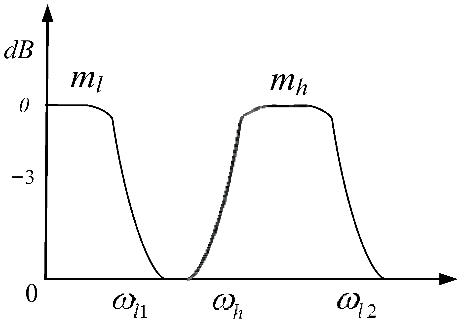
The line impedances are assumed to be mainly inductive in this paper. The power flow between two nodes can be expressed as:

$$P=\frac{E_1{E}_2}{X}\delta$$

(1)

$$Q=\frac{E_1\left(E_1-E_2\right)}{X},$$

(2)

where $E_1$ and $E_2$ are the voltage amplitudes, δ is the phase angle difference, and $X$ is the line impedance. From the two equations, it can be informed that the real power is proportional to $\delta$; and the reactive power is determined by the difference between $E_1$ and $E_2$ with fixed line impedance.

Using the $dq$ theory, the instantaneous output power $p$ and $q$, are given by

$$p=v_{od}{i}_{od}+v_{oq}{i}_{oq}$$

(3)

$$q=v_{od}{i}_{oq}-v_{oq}{i}_{od}.$$

(4)

The power controller received the measured output power through a low pass filter (LPF), which can be expressed as:

$$P=\frac{{\omega }_f}{s+{\omega }_f}p$$

(5)

$$Q=\frac{{\omega }_f}{s+{\omega }_f}q,$$

(6)

where ${\omega }_f$ is the cut-off frequency.

The conventional droop control scheme can be expressed as:

$$\omega ={\omega }^{\ast }-m_p\left(P-P^{\ast }\right)$$

(7)

$$V=V^{\ast }-n_q\left(Q-Q^{\ast }\right),$$

(8)

where $\omega$ and $V$ are the angular velocity and amplitude of the output voltage, ${\omega }^{\ast }$ and $V^{\ast }$ are the reference values, $P^{\ast }$ and $Q^{\ast }$ are the reference values of active and reactive power, and $m_p$ and $n_q$ are the active and reactive power droop coefficients, respectively.

The active power output is adjusted by the frequency. However, it is directly determined by the phase angular and not the frequency from Equation (1). The relation between them is

$$\Delta \delta =\frac{1}{s}\Delta \omega .$$

(9)

From Equation (8), it can be seen that the amplitude difference is necessary for reactive power sharing. However, $\Delta \omega$ is not necessary theoretically. The relationship between them in the steady state can be expressed as:

$$\Delta \omega =-m_p\Delta P$$

(10)

$$\Delta V=-n_q\Delta Q,$$

(11)

where $\Delta V=V-V^{\ast }$, $\Delta P=P-P^{\ast }$ and $\Delta Q=Q-Q^{\ast }$.

2.2. Washout Filter

The washout filter controller is a BPF without the low frequency component and can eliminate the frequency and amplitude deviations of output voltage in theory. As explained in [10], the control mechanism of the washout filter controller could be expressed as:

$$\omega ={\omega }^{\ast }-m_p·\frac{s}{s+{\omega }_h}·\left(P-P^{\ast }\right)$$

(12)

$$V=V^{\ast }-n_q·\frac{s}{s+{\omega }_h}·\left(Q-Q^{\ast }\right),$$

(13)

where ${\omega }_h$ is the cut-frequency of the high pass filter (HPF). By examining Equations (5), (6), (12) and (13), it can be derived that the following equation should be satisfied.

$${\omega }_h<{\omega }_f.$$

(14)

From Equations (5), (6), (12) and (13), the washout filter is a BPF indeed, as explained in [11]. When a load change happens, the selected frequency signals can be used by each DG to adjust its output power which is proportional to the droop coefficients $m_p$ and $n_q$. To remove the low-frequency signals, the last parts of Equations (12) and (13) should be zero theoretically in the steady state. Compared to the droop controller, the washout filter will not lead to frequency and amplitude deviation. It can achieve active power sharing at the same time. However, the lack of low-frequency signals leads to its inability to “plug and play”, which is shown in Section 6.

Equation (2) shows that the reactive power sharing relies on voltage amplitudes deviation between different nodes. If the amplitude restores to the rated value for each DG, there will be no amplitude deviation between each DG, and the reactive power output will be inversely proportional to the line impedance value if the network topology is star [22,23], which indicates that the washout filter controller does nothing on reactive power sharing in the steady state.

3. Proposed Control Strategy

As explained in Section 2, the conventional droop can achieve power sharing and “plug and play” but with frequency and amplitude differences of the output voltage. The washout filter can easily eliminate the frequency and amplitude differences, but with poor reactive power sharing and cannot realize “plug and play”. Inspired by this, a novel control strategy which combines the two control strategies together is proposed in this part, as shown in Figure 1. The droop control loop consists of an LPF, which makes it maintain the “plug and play” advantage, and the washout filter control loop aims to compensate the APDP caused by the small droop coefficient. Thus, the control scheme of the DWC can be derived as:

$$\omega ={\omega }^{\ast }-m_l·\left(P_1-P^{\ast }\right)-m_h·\frac{s}{s+{\omega }_h}·\left(P_2-P^{\ast }\right),$$

(15)

where $P_1=\frac{{\omega }_{l1}}{s+{\omega }_{l1}}p$, $P_2=\frac{{\omega }_{l2}}{s+{\omega }_{l2}}p$, $m_l$ is the droop coefficient, and $m_h$ is the washout filter coefficient. The DWC consists of two independent frequency bands whose frequency characteristics are shown in Figure 2. It should be noted that there is no size relationship between ${\omega }_{l1}$ and ${\omega }_h$. When ${\omega }_h={\omega }_{l1}$ and ${\omega }_{l2}\gg {\omega }_{l1}$, the DWC degenerates to a PD (proportional–differential) control method [6,9], where the differential coefficient is $\raisebox{1ex}{$m_h$}\!\left/ \!\raisebox{-1ex}{${\omega }_h$}\right.$.

Regardless of the difference between ${\omega }_{l1}$ and ${\omega }_{l2}$ and combined with Equation (1), Equation (15) can be rewritten as:

$$\omega -{\omega }^{\ast }=-m_l·\left(P_1-P^{\ast }\right)-\frac{1}{{\omega }_h}·\frac{d\omega }{dt}-\frac{m_l+m_h}{{\omega }_h}·\frac{E_1{E}_2}{X}·\left(\omega -{\omega }_g\right),$$

(16)

where ${\omega }_g$ is the frequency of the MG. Comparing Equation (16) and the virtual synchronous generator control equation in [24], which can be expressed as:

$$\omega -{\omega }^{\ast }=-m_l·\left(P_{\mathrm{out}}-P^{\ast }\right)-J{m}_l\omega \frac{d\omega }{dt}-D{m}_l·\left(\omega -{\omega }_g\right),$$

(17)

where $J$ is the virtual inertia and $D$ is the damping factor, it can be derived that

$$\{\begin{array}{l}J=\frac{1}{\omega m_l{\omega }_h}\hfill \\ D=\frac{1+\raisebox{1ex}{$m_h$}\!\left/ \!\raisebox{-1ex}{$m_l$}\right.}{{\omega }_h}·\frac{E_1{E}_2}{X}\hfill \end{array}.$$

(18)

Thus, the APDP of the DWC can be adjusted by tuning ${\omega }_h$ and $m_h$ [25].

With the analysis above, the correspondence between different control strategies can be summarized as:

• The “P-f” droop control strategy is equivalent to J = 0 and D = 0 [24].
• The “PD” control strategy [5,6,7,8,9] is equivalent to J = 0 with $D=\frac{m_h}{m_l}·\frac{E_1{E}_2}{X}$.
• The washout filter control [10] is equivalent to removing the parameter $m_l$.
• The DWC is equivalent to the “PD” controller with ${\omega }_h={\omega }_{l1}$ and ${\omega }_{l2}\gg {\omega }_{l1}$.
• The DWC is equal to the virtual synchronous generator control strategy with ${\omega }_{l2}={\omega }_{l1}$.

Since the washout filter cannot reduce amplitude difference, the reactive power controller adopts the conventional $Q-V$ droop controller as follows:

$$V=V^{\ast }-n_l·\left(Q-Q^{\ast }\right),$$

(19)

where $Q=\frac{{\omega }_{l1}}{s+{\omega }_{l1}}q$, and $n_l$ is the reactive power control loop coefficient.

The coefficient $m_l$ of each inverter should be set as [26]:

$$m_{l,i}\Delta P_i=m_{l,j}\Delta P_j.$$

(20)

Considering the APDP of the inverters, the same rule applies to coefficient $m_h$

$$m_{h,i}\Delta P_i=m_{h,j}\Delta P_j.$$

(21)

Since the frequency difference in the steady state has nothing to do with washout filter, it only relies on the droop controller. To reduce the frequency difference in the steady state, the value of $m_l$ should be set smaller compared to the conventional droop controller. However, small droop gain always leads to slow dynamic adjustment process, which is not desired. As analyzed above, the DWC can be seen as a virtual synchronous generator controller, so the APDP can be compensated by regulating ${\omega }_h$ and $m_h$.

The inner control loop includes a voltage controller which is a PI (proportional–integral) regulator and a current controller which is a P regulator.

4. Small Signal Model

The small signal model of an islanded MG embedded with the DWC is constructed as a singular system in this section. Based on the model, the stability is analyzed. Before modeling, some symbols need to be defined. Suppose the system has “m” nodes, “s” inverters, “n” lines, and “p” load points [12]. The complete model consists of a differential algebraic part and an algebraic part. Since the differential equations has been discussed by many articles [4,12,13,14,15], the details of some matrices are given in Appendix A and not repeat in each section.

4.1. Differential Algebraic Equations

4.1.1. Load and Network Models

The state equations of loads which are general resistive and inductive loads are expressed as follows:

$$\begin{array}{cc}\hfill E_{LOAD}\dot{\left[\Delta i_{loadDQ}\right]}& =A_{LOAD}\left[\Delta i_{loadDQ}\right]+B_{1LOAD}\left[\Delta v_{bDQ}\right]+B_{2LOAD}\left[\Delta \omega \right]\hfill \\ \hfill \left[\Delta i_{loadDQ}\right]& =C_{LOAD}\left[\Delta i_{loadDQ}\right]\hfill \\ \hfill \left[\Delta v_{bDQ}\right]& =\left[\begin{array}{cccc}\Delta v_{bDQ,1}& \Delta v_{bDQ,2}& \cdots & \Delta v_{bDQ,m}\end{array}\right],\hfill \end{array}$$

(22)

where $E_{LOAD}$ is a unit matrix of 2p-dimensions and $C_{load}$ is a unit matrix of 2p-dimensions, too.

The model of the network can be represented by the following equations:

$$\begin{array}{cc}\hfill E_{NET}\dot{\left[\Delta i_{lineDQ}\right]}& =A_{NET}\left[\Delta i_{lineDQ}\right]+B_{1NET}\left[\Delta v_{bDQ}\right]+B_{2NET}\left[\Delta \omega \right]\hfill \\ \hfill \left[\Delta i_{lineDQ}\right]& =C_{line}\left[\Delta i_{lineDQ}\right],\hfill \end{array}$$

(23)

where $E_{NET}$ and $C_{line}$ are two unit matrixes of 2n-dimensions.

4.1.2. Singular Inverter Model

Power Controller: To model the power controller, Equation (15) needs to be rewritten as:

$$\Delta \mathsf{\omega }=\Delta {\mathsf{\omega }}_1+\Delta {\mathsf{\omega }}_2,$$

(24)

where $\Delta {\mathsf{\omega }}_1=-m_l·\Delta P_1$, and $\Delta {\mathsf{\omega }}_2=-m_h·\frac{s}{s+{\omega }_h}·\Delta P_2$. Combining with Equation (9), the relations between the power angles and active power variables can be expressed as [27]:

$$\{\begin{array}{l}\Delta {\mathsf{\delta }}_1=-\frac{m_l}{s}·\Delta P_1\hfill \\ \Delta {\mathsf{\delta }}_2=-m_h·\frac{1}{s+{\omega }_h}·\Delta P_2\hfill \end{array}.$$

(25)

By linearizing Equations (19) and (25), the model of the power controller can be expressed as:

$$\begin{array}{cc}\hfill E_P\dot{\left[\Delta x_p\right]}& =A_P\left[\Delta x_p\right]+B_P\left[\begin{array}{c}\Delta i_{ldq}\\ \Delta v_{odq}\\ \Delta i_{oDQ}\end{array}\right]+B_{P\omega com}\left[\Delta {\omega }_{com}\right]\hfill \\ \hfill \left[\Delta v_{odq}^{\ast }\right]& =C_{PV}\left[\Delta x_p\right]\hfill \\ \hfill \left[\Delta \omega \right]& =C_{P\omega }\left[\Delta x_p\right]\hfill \end{array}.$$

(26)

In Equation (26),

$$\left[\Delta x_p\right]={\left[\begin{array}{ccccc}\Delta {\delta }_1& {\Delta }_2& \Delta P_1& \Delta P_2& \Delta Q\end{array}\right]}^T.$$

(27)

Voltage and Current Controllers: As the voltage controller is a PI regulator and the current is a P regulator, they are formulated together for convenience:

$$\begin{array}{cc}\hfill E_{VC}\dot{\left[\Delta {\varnothing }_{dq}\right]}& =\left[0\right]\left[\Delta {\varnothing }_{dq}\right]+B_{VC1}\left[\Delta v_{odq}^{\ast }\right]+B_{VC2}\left[\begin{array}{c}\Delta i_{ldq}\\ \Delta v_{odq}\\ \Delta i_{oDQ}\end{array}\right]\hfill \\ \hfill \left[\Delta v_{idq}^{\ast }\right]& =C_{VC}\left[\Delta {\varnothing }_{dq}\right]+D_{VC1}\left[\Delta v_{odq}^{\ast }\right]+D_{VC2}\left[\begin{array}{c}\Delta i_{ldq}\\ \Delta v_{odq}\\ \Delta i_{oDQ}\end{array}\right],\hfill \end{array}$$

(28)

LCL Filter: The LCL filter can be modeled as follows:

$$E_{LCL}\dot{\left[\Delta x_{lcl}\right]}=A_{LCL}\left[\Delta x_{lcl}\right]+B_{LCL1}\left[\Delta v_{idq}\right]+B_{LCL2}\left[\Delta v_{bDQ}\right]+B_{LCL3}\left[\Delta \omega \right]$$

(29)

In Equation (29),

$$\left[\Delta x_{lcl}\right]={\left[\begin{array}{ccc}\Delta i_{ldq}& \Delta v_{odq}& \Delta i_{odq}\end{array}\right]}^T.$$

(30)

Common Frame Transformation: For the convenience of system modeling, the small signal model of each inverter can be built separately. Every DG’s dq transformation is on its local reference frame ($d-q$). However, the output variables of each component should be converted to the common reference frame ($D-Q$) to construct a whole system, and the transformation equations for these variables could be written as [12]:

$$\left[\Delta i_{oDQ}\right]=T_S\left[\Delta i_{odq}\right]+T_C\left[\Delta \delta \right]$$

(31)

$$\left[\Delta v_{bdq}\right]=T_S^{-1}\left[\Delta v_{oDQ}\right]+T_V^{-1}\left[\Delta \delta \right].$$

(32)

Complete Model of an Individual Inverter: The complete model of an individual inverter consists of the circuit part and the controller part which has 13 state variables. The complete model of an inverter can be expressed as:

$$\begin{array}{cc}\hfill E_{INVi}\dot{\left[\Delta x_{invi}\right]}& =A_{INVi}\left[\Delta x_{invi}\right]+B_{INVi}\left[\Delta v_{bDQi}\right]+B_{i\omega com}\left[\Delta {\omega }_{com}\right]\hfill \\ \hfill \left[\begin{array}{c}\Delta \omega \\ \Delta i_{oDQi}\end{array}\right]& =\left[\begin{array}{c}{C}_{INVwi}\\ C_{INVci}\end{array}\right]\left[\Delta x_{invi}\right],\hfill \end{array}$$

(33)

where

$$\left[\Delta x_{invi}\right]={\left[\begin{array}{ccc}\Delta x_{pi}& \Delta {\varnothing }_{dqi}& \Delta x_{lcli}\end{array}\right]}^{\mathrm{T}}.$$

(34)

4.1.3. Combined Model of All Inverters

As an individual model of an inverter has been built, the combined model of all inverters in an islanded MG can be expressed as follows:

$$\begin{array}{cc}\hfill E_{INV}\dot{\left[\Delta x_{INV}\right]}& =A_{INV}\left[\Delta x_{INV}\right]+B_{INV}\left[\Delta v_{bDQ}\right]\hfill \\ \hfill \left[\Delta i_{oDQ}\right]& =C_{INVc}\left[\Delta x_{INV}\right],\hfill \end{array}$$

(35)

where

$$\left[\Delta x_{INV}\right]={\left[\begin{array}{cc}\begin{array}{cc}\Delta x_{inv,1}& \Delta x_{inv,2}\end{array}& \begin{array}{cc}\cdots & \Delta x_{inv,s}\end{array}\end{array}\right]}^T.$$

(36)

4.2. Algebraic Equations

Using Kirchhoff’s current law (KCL) for each node, it is easy to derive that

$$\left[0\right]\left[\Delta v_{bDQ,i}\right]=\left[\Delta i_{oDQ,i}\right]-\left[\Delta i_{loadDQ,i}\right]+{{\displaystyle \sum }}_{jϵG}\left[\Delta i_{lineDQ,ji}\right],$$

(37)

where G is a set which contains the nodes connected to node i, and $\Delta v_{bDQ,i}$ are algebraic variable.

Applying this relation to all nodes in the system, it can be obtained that

$$M_{INV}\left[\Delta i_{oDQ}\right]+M_{NET}\left[\Delta i_{lineDQ}\right]+M_{LOAD}\left[\Delta i_{loadDQ}\right]=0,$$

(38)

where $M_{INV}$, $M_{NET}$ and $M_{LOAD}$ are the mapping matrix of the network structure of the system and are detailed defined in [12].

4.3. Complete Microgrid (MG) Model

By combing all of the inverters, loads, distribution lines and the relations of coupling states, the complete state matrix of an MG can be obtained as:

$$E_{sys}\dot{\left[\Delta x_{sys}\right]}=A_{sys}\left[\Delta x_{sys}\right],$$

(39)

where

$$\left[\Delta x_{sys}\right]=\left[\begin{array}{cccc}\Delta x_{INV}& \Delta i_{lineDQ}& \Delta i_{loadDQ}& \Delta v_{bDQ}\end{array}\right]$$

(40)

$$\begin{array}{l}{E}_{sys}=\left[\begin{array}{cccc}{E}_{INV}& 0& 0& 0\\ 0& E_{NET}& 0& 0\\ 0& 0& E_{LOAD}& 0\\ 0& 0& 0& 0_{2m\times 2m}\end{array}\right]\hfill \\ A_{sys}=\left[\begin{array}{cccc}{A}_{INV}& 0& 0& B_{INV}\\ B_{2NET}{C}_{INV\omega }& A_{NET}& 0& B_{1NET}\\ B_{2LOAD}{C}_{INV\omega }& 0& A_{LOAD}& B_{1LOAD}\\ M_{INV}{C}_{INVc}& M_{NET}{C}_{line}& M_{LOAD}{C}_{LOAD}& 0_{2m\times 2m}\end{array}\right].\hfill \end{array}$$

(41)

The matrix $E_{sys}$ is singular obviously, which indicates that the system is a singular system.

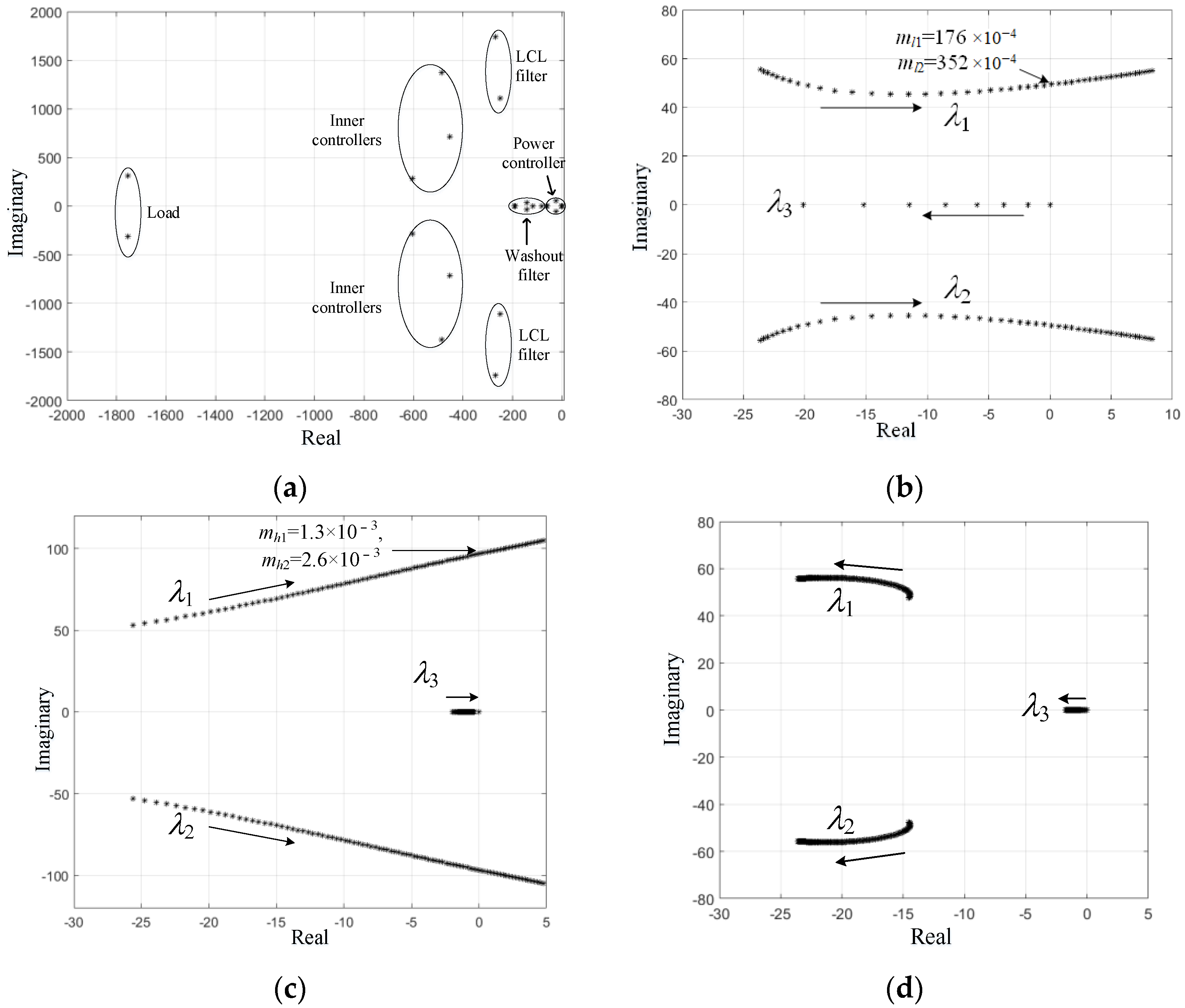
5. Stability Analysis

The small signal model built in Section 4 is singular. To analyzed the system, a determinant is defined as:

$$\Delta \left(\mathrm{s}\right):=\left|\mathrm{s}{E}_{sys}-A_{sys}\right|.$$

(42)

The stability of the system is determined by the roots of $\Delta \left(\mathrm{s}\right)$. A simple method to observe the stability of the system is checking whether the real parts of all its finite eigenvalues are negative. If all are negative, the system is stable [28]. The pencil ($\mathrm{s}{E}_{sys}-A_{sys}$) is regular when $\Delta \left(\mathrm{s}\right)$ is not identically zero. The model of an MG is always regular since it is a physical dynamical system [29].

In this paper, ${\mathrm{DG}}_1$ is chosen as the common reference frame, so $\Delta {\delta }_1$ and $\Delta {\delta }_2$ in ${\mathrm{DG}}_1$ are ignored in calculation [15]. The eigenvalues can be easily calculated with function “eig(A,B)” in MATLAB (MathWorks, Natick, MA, USA), where “A” corresponds to $A_{sys}$, and “B” corresponds to $E_{sys}$.

In this section, the MG shown in Figure 1 is analyzed. Its complete model is constructed using the procedure shown in Section 4. The eigenvalues of the system can be found using the method described above. The parameters of the MG are shown in

Table 1. Test System Parameters.

Parameter	Value	Parameter	Value
$V_{DC}$	800 V	$f_s$	5 kHz
$m_{l1}$	$6.3\times {10}^{-6}$	$V_g$	380 V (line-line)
$m_{h1}$	$6\times {10}^{-5}$	$r_{L_f}$	0.1 Ω
$n_{l1}$	0.001	$L_f$	1 mH
${\omega }_{l1}$	20 π rad/s	$C_f$	800 μF
${\omega }_{l2}$	60 π rad/s	$r_{L_c}$	0.03 Ω
${\omega }_h$	40 π rad/s	$L_c$	0.3 mH
$K_{pv}$	0.1	${\omega }_0$	50 Hz
$K_{iv}$	150	$r_{line,1}$	0.12 Ω
$K_{pc}$	0.002	$L_{line,1}$	1.2 mH
$R_{load}$	10 Ω	$r_{line,2}$	0.08 Ω
$L_{load}$	5 mH	$L_{line,2}$	0.8 mH

, and the steady points, which are measured from a MATLAB/SIMULINK simulation, of the MG are summarized in

Table 2. Initial Conditions.

Parameter	Value	Parameter	Value
$V_{od}$	(10.0 309.5)	$V_{oq}$	(0 0)
$I_{od}$	(20.0 10.1)	$I_{oq}$	(−1.2 −4.2)
$I_{ld}$	(20.0 10.1)	$I_{lq}$	(76.6 73.2)
$V_{bd}$	(309.6 309.2 307.5)	$V_{bq}$	(29.6 27.6 23.9)
$I_{lined}$	(20.0 10.1)	$I_{lineq}$	(−0.81 −3.4)
${\delta }_0$	(−0.2 0)	$I_{loadq}$	(30.3 −2.6)

.

The root loci of the system are shown in Figure 3. Figure 3a is the eigenvalues for the parameters given in Table 2. The eigenvalues labeled Load are mainly affected by the load parameters. The modes labeled Inner controllers are sensitive to the voltage and current controllers. In the group labeled LCL filter, the modes are associated with the LCL filter parameters. The modes shown in Power controller group are sensitive to the power controller parameters. The modes labeled Washout filter are associated with the frequency parameters of the washout filter. Since the parameter ${\omega }_{l2}$ has little effect on the dominant poles, the root locus is not shown here.

Figure 3b shows the trajectory of the three dominant poles as the droop coefficients $m_{l1}$ changes from $6\times {10}^{-6}$ to $6\times {10}^{-4}$, where $m_{l2}$ is always two times of $m_{l1}$. The influence of ${\lambda }_1$ and ${\lambda }_2$ is easily analyzed. ${\lambda }_3$ could be seen as an inertial link. When droop coefficients increase, the eigenvalues ${\lambda }_1$ and ${\lambda }_2$ move towards vertical axis and the eigenvalue ${\lambda }_3$ moves away from it, which improve the dynamic performance of the system, but oversized droop coefficients cause system oscillation and instability.

Figure 3c shows the root locus of $m_{h1}$ as it moves from 0 to $1.4\times {10}^{-3}$, where $m_{h2}$ is always two times $m_{h1}$. When $m_{h1}$ increases, the three dominate poles move close to the imaginary axis. On the one hand, ${\lambda }_1$ and ${\lambda }_2$ increase the dynamic performance of the system but make it more oscillatory. On the other hand, ${\lambda }_3$ suppresses the oscillation but increases the adjustment time of the system. To improve the dynamic performance, ${\lambda }_1$ and ${\lambda }_2$ should be set close to the imaginary axis.

Figure 3d shows the root locus of ${\omega }_h$ as it moves from 0 to 125.6, which results in the dominant poles moving away from the imaginary axis. Considering Figure 3c,d, the ${\lambda }_1$ and ${\lambda }_2$ could have more flexible assignment by adjusting parameters ${\omega }_h$ and $m_h$. Thus, the larger ${\omega }_h$ is, the faster the dynamic performance is. However, considering the impact on the inner control loop, it is set as 40 π in this paper. There is another design shown in the next section. In that design, ${\omega }_h$ should be set very small, and $m_h$ is several times $m_l$.

To sum up, the droop coefficient $m_l$ could be set smaller compared to the conventional principle to reduce the frequency difference in the steady state, and the washout filter could be added to compensate the APDP.

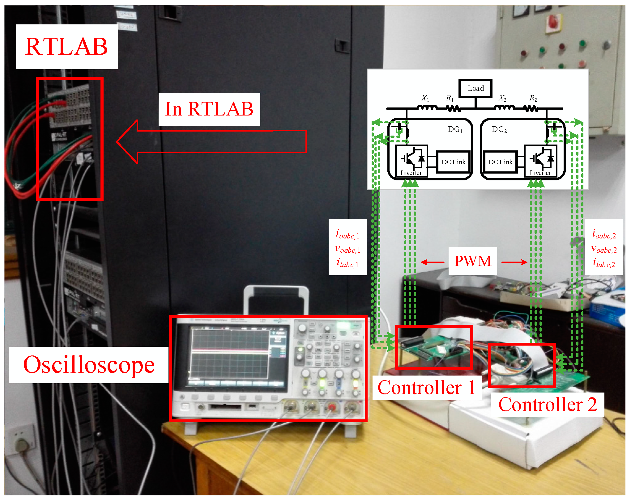
6. Real Time Simulation Results

The DWC is verified in real-time simulations with HIL [30]. The MG shown in Figure 1 is simulated in RT-LAB (Opal-RT, Montreal, QC, Canada) and the controllers run in STM32F407 MCUs (STMicroelectronics, Geneva, Switzerland). The real-time simulation apparatus is shown in Figure 4.

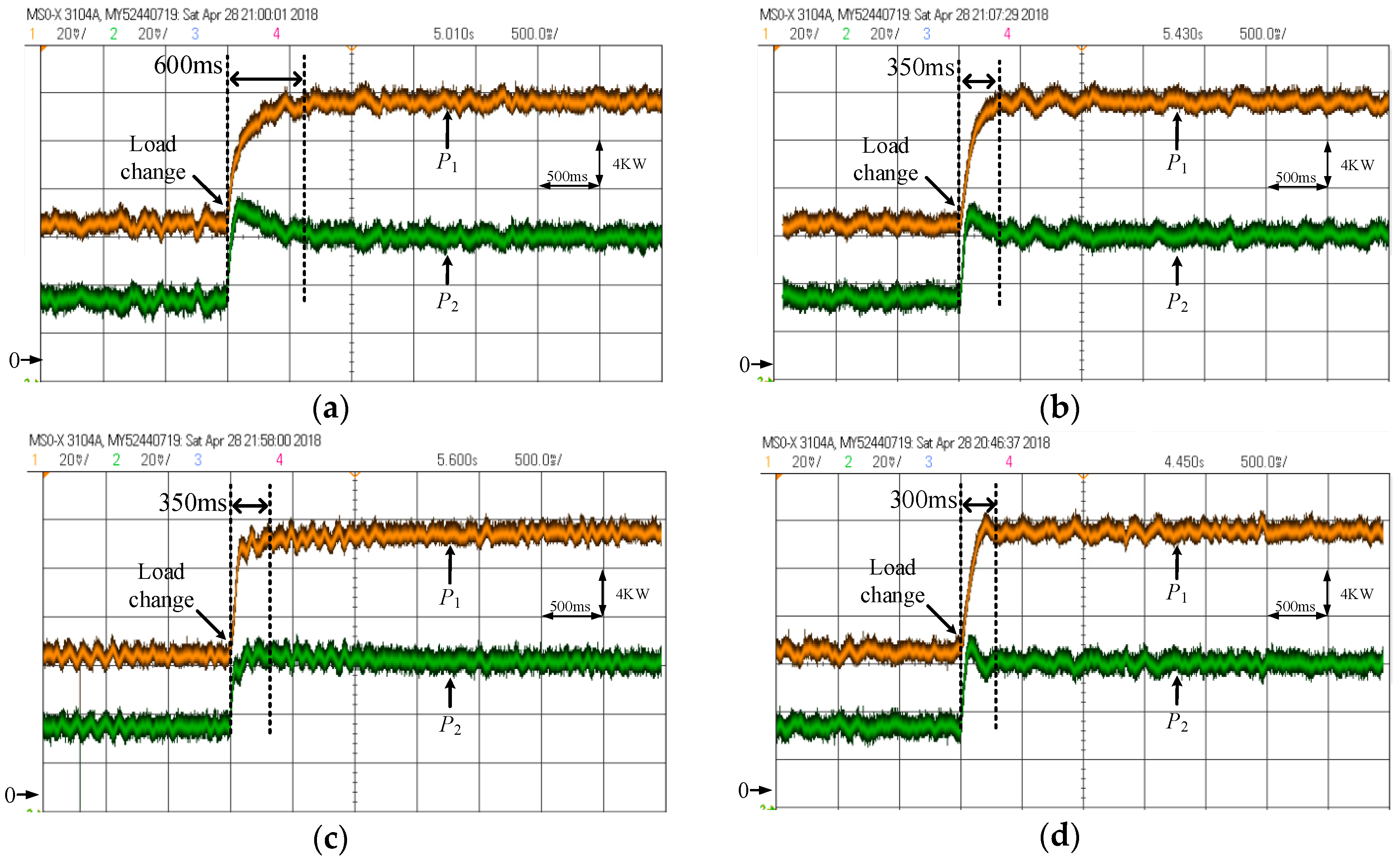
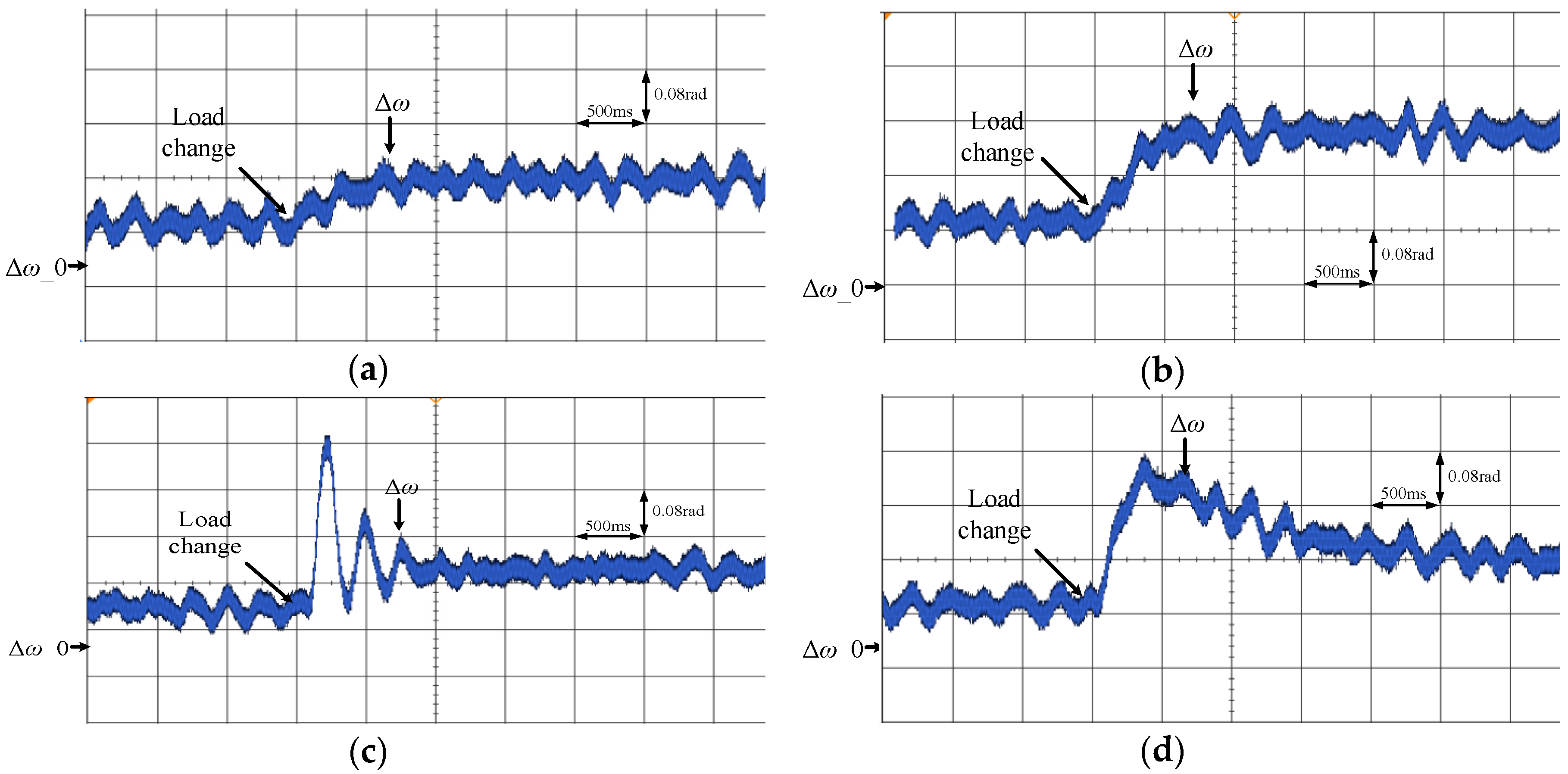
6.1. Performance Comparison with the Conventional Droop Controller

To verify the DWC on APDP and frequency deviation compared to the conventional droop control strategy, the performances of the two control strategies are compared in this section. Different frequency ranges are selected of the washout filter to shown the performance of the DWC. The active power performance is presented in Figure 5 and the corresponding frequency performance is presented in Figure 6, which is defined as:

$$\Delta \omega ={\omega }_0-\omega .$$

(43)

The parameters are listed in Table 1. The droop coefficients of the active power control loop for the two DGs are set as 6.3 $\times {10}^{-6}$ and 12.6 $\times {10}^{-6}$ in the three cases. Initially, the MG is in steady state. At t = 1.5 s, a resistive load of 15 kW is connected to the MG. Figure 5a shows the performance of droop control method. The droop coefficients in Figure 5b is two times of Figure 5a. Figure 5c shows the performance in which the washout filters coefficients ${\omega }_h$ and ${\omega }_{l2}$ are set as 40 π and 60 π, $m_{h1}$ and $m_{h2}$ are set as 5 $\times {10}^{-4}$ and 1 $\times {10}^{-3}$, respectively. In Figure 5d, ${\omega }_h$ and ${\omega }_{l2}$ are set as 0.4π and 20π and $m_{h1}$ and $m_{h2}$ are set as 1.9 $\times {10}^{-5}$ and 3.8 $\times {10}^{-5}$. The results are listed in

Table 3. Dynamic performance.

Figure 5 and Figure 6	a	b	c	d
Adjustment Time (ms)	600	350	350	300
Overshoot (%, DG2)	23	15	10	15
Frequency deviation (rad)	0.08	0.16	0.08	0.08

. In Figure 5a,b, it can be seen that the APDP can be improved by increasing the droop coefficient, but it also increases the frequency deviation in Figure 6a,b.

In Figure 5c, the washout filter is designed in high-frequency band. As analyzed in Section 5, the eigenvalues are close to the imaginary axis in this design, which means the dynamic performance of the system is fast. In Figure 5d, the washout filter is designed in low-frequency band. Although the eigenvalue distribution is similar, the virtual inertia and damping factor are bigger compared with Figure 5c. Figure 6c,d shows the corresponding frequency dynamic performances. In Figure 6c, the frequency changes rapidly, as parameter ${\omega }_h$ is large (small virtual inertia). Conversely, the frequency changes slowly in Figure 6d, as ${\omega }_h$ is small (large virtual inertia). In Figure 5 and Figure 6, it can be seen that the system using he DWC can achieve a better APDP with the same frequency deviation in the steady state compared to the droop controller.

6.2. Performance Comparison with the Washout Filter Controller

The “plug-and-play” capabilities of the washout filter controller and the DWC are shown in Figure 7 and Figure 8. The parameters of the washout filter are ${\omega }_h=0.4\mathsf{\pi }\mathrm{and}$ ${\omega }_{l2}=20\mathsf{\pi }$. The coefficients are $m_{l1}=1\times {10}^{-6}$, $m_{l2}=2\times {10}^{-6}, m_{h1}=2\times {10}^{-6}$, and $m_{h2}=4\times {10}^{-6}$.

In Figure 7, there is only a washout filter control loop in the power controller. From t = 0 s to t = 10 s, the system is under steady state. The output power of the two DGs are 9 kW and 6 kW, respectively, the ratio of which does not meet the designed 2:1. At t = 10 s, DG₂ is disconnected from the MG and, at t = 20 s, the synchronization process starts. When the angular and voltage amplitude meets the requirements, DG₂ is reconnected to the MG. At this moment, the active power outputs are 13 kW and 2 kW, respectively. The operating point does not meet the requirement and is different with the operating point from 0 s to 10 s. Figure 7 shows the washout filter is weak on “plug-and-play” for the lack of static component. Figure 8 shows that the output power of the two DGs are 10 kW and 5 kW from 0 s to 10 s and from 30 s to 50 s, respectively, which indicates the sharing is accurate both before the line disconnection and after the line reconnection. Figure 8 verifies the “plug-and-play” capabilities of the DWC.

7. Conclusions

In this paper, an improved droop control strategy that combines the droop controller and washout filter controller is proposed, obtaining the advantages of both. The DWC can achieve “plug-and-play” with the droop control loop, and the washout filter controller is used to improve the APDP. The droop gains could be small to reduce the frequency difference in the steady state, and the washout filter is to compensate the APDP loss in this paper. In addition, a complete singular small signal model of an MG using the DWC is rebuilt. Using the singular model, the stability of the system is discussed. Finally, an MG embedded with the DWC has been tested with HIL, which demonstrates the effectiveness of the DWC on frequency deviation and APDP.

References

1. Hossain, A.M.; Pota, R.H.; Issa, W.; Hossain, J.M. Overview of AC Microgrid Controls with Inverter-Interfaced Generations. Energies 2017, 10, 1300. [Google Scholar] [CrossRef]
2. Li, D.; Zhao, B.; Wu, Z.; Zhang, X.; Zhang, L. An Improved Droop Control Strategy for Low-Voltage Microgrids Based on Distributed Secondary Power Optimization Control. Energies 2017, 10, 1347. [Google Scholar] [CrossRef]
3. Dou, C.; Zhang, Z.; Yue, D.; Gao, H. An Improved Droop Control Strategy Based on Changeable Reference in Low-Voltage Microgrids. Energies 2017, 10, 1080. [Google Scholar] [CrossRef]
4. Zhang, H.; Kim, S.; Sun, Q.; Zhou, J. Distributed Adaptive Virtual Impedance Control for Accurate Reactive Power Sharing Based on Consensus Control in Microgrids. IEEE Trans. Smart Grid 2016. [Google Scholar] [CrossRef]
5. Mohamed, Y.A.R.I.; El-Saadany, E.F. Adaptive Decentralized Droop Controller to Preserve Power Sharing Stability of Paralleled Inverters in Distributed Generation Microgrids. IEEE Trans. Power Electron. 2008, 23, 2806–2816. [Google Scholar] [CrossRef]
6. Kim, J.; Guerrero, J.M.; Rodriguez, P.; Teodorescu, R.; Nam, K. Mode Adaptive Droop Control With Virtual Output Impedances for an Inverter-Based Flexible AC Microgrid. IEEE Trans. Power Electron. 2011, 26, 689–701. [Google Scholar] [CrossRef]
7. Mohamed, Y.A.-R.I.; Radwan, A.A. Hierarchical Control System for Robust Microgrid Operation and Seamless Mode Transfer in Active Distribution Systems. IEEE Trans. Smart Grid 2011, 2, 352–362. [Google Scholar] [CrossRef]
8. Chen, J.; Wang, L.; Diao, L.; Du, H.; Liu, Z. Distributed Auxiliary Inverter of Urban Rail Train—Load Sharing Control Strategy under Complicated Operation Condition. IEEE Trans. Power Electron. 2016, 31, 2518–2529. [Google Scholar] [CrossRef]
9. Xia, Y.; Peng, Y.; Wei, W. Triple droop control method for ac microgrids. IET Power Electron. 2017, 10, 1705–1713. [Google Scholar] [CrossRef]
10. Yazdanian, M.; Mehrizi-Sani, A. Washout Filter-Based Power Sharing. IEEE Trans. Smart Grid 2015. [Google Scholar] [CrossRef]
11. Han, Y.; Li, H.; Xu, L.; Zhao, X.; Guerrero, J. Analysis of Washout Filter-Based Power Sharing Strategy—An Equivalent Secondary Controller for Islanded Microgrid without LBC Lines. IEEE Trans. Smart Grid 2017. [Google Scholar] [CrossRef]
12. Pogaku, N.; Prodanovic, M.; Green, T.C. Modeling, Analysis and Testing of Autonomous Operation of an Inverter-Based Microgrid. IEEE Trans. Power Electron. 2007, 22, 613–625. [Google Scholar] [CrossRef]
13. Bottrell, N.; Prodanovic, M.; Green, T.C. Dynamic Stability of a Microgrid with an Active Load. IEEE Trans. Power Electron. 2013, 28, 5107–5119. [Google Scholar] [CrossRef]
14. Rasheduzzaman, M.; Mueller, J.A.; Kimball, J.W. An Accurate Small-Signal Model of Inverter- Dominated Islanded Microgrids Using $dq$ Reference Frame. IEEE J. Emerg. Sel. Top. Power Electron. 2014, 2, 1070–1080. [Google Scholar] [CrossRef]
15. Rasheduzzaman, M.; Mueller, J.A.; Kimball, J.W. Reduced-Order Small-Signal Model of Microgrid Systems. IEEE Trans. Sustain. Energy 2015, 6, 1292–1305. [Google Scholar] [CrossRef]
16. Leitner, S.; Yazdanian, M.; Mehrizi-Sani, A.; Muetze, A. Small-Signal Stability Analysis of an Inverter-Based Microgrid with Internal Model–Based Controllers. IEEE Trans. Smart Grid 2017. [Google Scholar] [CrossRef]
17. Yu, K.; Ai, Q.; Wang, S.; Ni, J.; Lv, T. Analysis and Optimization of Droop Controller for Microgrid System Based on Small-Signal Dynamic Model. IEEE Trans. Smart Grid 2015. [Google Scholar] [CrossRef]
18. Mohammadi, F.D.; Keshtkar, H.; Feliachi, A. State Space Modeling, Analysis and Distributed Secondary Frequency Control of Isolated Microgrids. IEEE Trans. Energy Convers. 2017. [Google Scholar] [CrossRef]
19. Peng, Y.; Shuai, Z.; Shen, J.; Wang, J.; Tu, C.; Cheng, Y. Reduced order modeling method of inverter-based microgrid for stability analysis. In Proceedings of the 2017 IEEE Applied Power Electronics Conference and Exposition (APEC), Tampa, FL, USA, 26–30 March 2017; pp. 3470–3474. [Google Scholar]
20. Egwebe, A.M.; Fazeli, M.; Igic, P.; Holland, P.M. Implementation and Stability Study of Dynamic Droop in Islanded Microgrids. IEEE Trans. Energy Convers. 2016, 31, 821–832. [Google Scholar] [CrossRef]
21. Rosenbrock, H.H. Structural properties of linear dynamical systems. Int. J. Control 2007, 20, 191–202. [Google Scholar] [CrossRef]
22. Mahmood, H.; Michaelson, D.; Jiang, J. Reactive Power Sharing in Islanded Microgrids Using Adaptive Voltage Droop Control. IEEE Trans. Smart Grid 2015, 6, 3052–3060. [Google Scholar] [CrossRef]
23. Zhou, J.; Kim, S.; Zhang, H.; Sun, Q.; Han, R. Consensus-based Distributed Control for Accurate Reactive, Harmonic and Imbalance Power Sharing in Microgrids. IEEE Trans. Smart Grid 2016. [Google Scholar] [CrossRef]
24. Liu, J.; Miura, Y.; Ise, T. Comparison of Dynamic Characteristics between Virtual Synchronous Generator and Droop Control in Inverter-Based Distributed Generators. IEEE Trans. Power Electron. 2016, 31, 3600–3611. [Google Scholar] [CrossRef]
25. Nguyen, C.-K.; Nguyen, T.-T.; Yoo, H.-J.; Kim, H.-M. Improving Transient Response of Power Converter in a Stand-Alone Microgrid Using Virtual Synchronous Generator. Energies 2018, 11, 27. [Google Scholar] [CrossRef]
26. Guerrero, J.M.; Hang, L.; Uceda, J. Control of Distributed Uninterruptible Power Supply Systems. IEEE Trans. Ind. Electron. 2008, 55, 2845–2859. [Google Scholar] [CrossRef] [Green Version]
27. Sun, Y.; Hou, X.; Yang, J.; Han, H.; Su, M.; Guerrero, J.M. New Perspectives on Droop Control in AC Microgrid. IEEE Trans. Ind. Electron. 2017, 64, 5741–5745. [Google Scholar] [CrossRef] [Green Version]
28. Lewis, F.L. A survey of linear singular systems. Circuits Syst. Signal Process. 1986, 5, 3–36. [Google Scholar] [CrossRef]
29. Milano, F.; Dassios, I. Primal and Dual Generalized Eigenvalue Problems for Power Systems Small-Signal Stability Analysis. IEEE Trans. Power Syst. 2017, 32, 4626–4635. [Google Scholar] [CrossRef]
30. Cai, H.; Xiang, J.; Wei, W.; Chen, M.Z.Q. V-dp/dv Droop Control for PV Sources in DC Microgrids. IEEE Trans. Power Electron. 2017. [Google Scholar] [CrossRef]
Figure 1. The study microgrid (MG) and the droop washout filter controller (DWC). DC: direct-current; PWM: pulse width modulation; PI: proportional integral.
Energies 11 02415 g001
Figure 2. Frequency characteristics of the DWC.
Energies 11 02415 g002
Figure 3. Dominant root locus of the system: (a) eigenvalue spectrum of MG state matrix; (b) dominant root locus as m l 1 [ 6 × 10 6 , 6 × 10 4 ]; (c) dominant root locus as m h 1   [0, 1.4 × 10 3 ]; and (d) dominant root locus as ω h   [0, 125.6]. LCL: inductor-capacitor-inductor.
Energies 11 02415 g003
Figure 4. Hardware in the loop (HIL) simulation setup for the study system.
Energies 11 02415 g004
Figure 5. Active power sharing performance: (a) droop controller with m l 1 = 6.3 × 10 6 , m l 2 = 1.26 × 10 5 ; (b) droop controller with m l 1 = 1.26 × 10 5 , m l 2 = 2.52 × 10 5 ; (c) DWC with large ω h ; and (d) DWC with small ω h .
Energies 11 02415 g005
Figure 6. Frequency deviations performance: (a) droop controller with m l 1 = 6.3 × 10 6 , m l 2 = 1.26 × 10 5 ; (b) droop controller with m l 1 = 1.26 × 10 5 , m l 2 = 2.52 × 10 5 ; (c) DWC with large ω h ; and (d) DWC with small ω h .
Energies 11 02415 g006
Figure 7. Performance of the washout controller under feeder disturbance.
Energies 11 02415 g007
Figure 8. Performance of the DWC under feeder disturbance.
Energies 11 02415 g008