Reconstruction of Hydraulic Fractures Using Passive Ultrasonic Travel-Time Tomography

Abstract

The knowledge of hydraulic fracture morphology is significant for the analysis of fracture mechanisms. This paper utilizes passive Ultrasonic Travel-time Tomography (UTT) to characterize the hydraulic fracture. We constructed a velocity model based on X-ray computerized tomography (X-CT) images scanned on a real hydraulically fractured shale column. Then, ray-paths and travel times corresponding to the source-receiver configuration were calculated by curved ray-tracing schemes. Lastly, we performed tomographic inversions using total variation regularization (TVR). The simulation results showed that 3D passive UTT based on TVR is an accurate, efficient, and stable method to reconstruct the velocity structures with fractures, even in the case of sparse ray-coverage or high noise level. Meanwhile, we also verified that the passive UTT is a valid alternative to X-CT in depicting the hydraulic fracturing rock via a proper interpretation method.

1. Introduction

Hydraulic fracturing has been a well-known technique for shale gas development in the last decades [1]. As a method for studying its mechanisms, laboratory hydraulic fracture experiments have been extensively performed. The geometry of hydraulically induced fractures is especially significant in the analysis of the fracture mechanism. Usually, we can use the X-ray computerized tomography (X-CT) scanning technique to display and investigate the fracture morphology inside the rock [2,3,4,5]. However, X-CT is not an ideal tool due to its high cost, high radiation risk, and inconvenience for real-time monitoring. Given this, more and more attention has been paid to the techniques that can approximately replace X-CT to bypass these drawbacks while operating at a similar accuracy or resolution. One of the widely used techniques is the Ultrasonic Travel-time Tomography (UTT) technique. It has been used to investigate the hydraulically fractured process of granite [6], stress distribution of uniaxially loaded rock [7], and localized deformation in porous sandstones [8] and soft rocks [9]. We can also monitor the CO₂ injection into water-saturated porous sandstone [10] by using UTT. However, because a limited number of transmitting sensors can be set along the sample, the resolution of UTT is always very low. Fortunately, acoustic emission (AE) can also be utilized as passive sources of UTT to reveal the fracture growth process due to its high rates of occurrence during hydraulic fracturing. Shiotani et al. [11] verify the feasibility of 3D AE tomography in triaxial tests of rocky specimens. Yang et al. [12] also imaged the stress redistribution of granite before its failure via passive tomography. Although the failure of rock can generate amounts of AEs, there are always few receivers placed around a sample. That is to say, the sampling of UTT is usually deficient for Nyquist theorem (i.e., the sampling rate must be at least twice that of the Nyquist frequency [13]).

Nevertheless, UTT always has a lower resolution than X-CT because of high attenuation and scattering of ultrasound in the rock [14]. Hence, to better characterize the hydraulic fracture using UTT, we must find ways to enhance its resolution or reduce the loss of resolution. Generally, there are several methods to realize this. The first is to increase the dominant frequency (f_d) of the ultrasound, which is a physical method. However, the f_d of acoustic emission depends on the rock properties [15]. That is to say, it is not artificially controlled, so this method is not applicable for passive UTT. The second way is to improve the ray-coverage so we can get enough data to get high-resolution inversion results. Charalampidou [8] get high-resolution UTT images of porous sandstones with dense sampling by using multi-element ultrasonic transducer arrays. However, in most cases, we can only get under-sampling and insufficient data (e.g., the experiment conducted by Yang et al. [12]). Moreover, the sparse ray-coverage make the tomographic inversions ill-posed. One way to reduce the ill-posedness is the regularization technique [16]. This method stabilizes ill-posed inversion problems by including an additional regularization term to the data misfit term. The most classical regularization method is the Tikhonov-Regularization (Tikh) [17]. However, due to the quadratic term used in the Tikh, its solution is always over-smoothed [16], which goes against the description of the fractures. Therefore, a new method is desperately needed to decrease the resolution loss induced by the limited-view. Fortunately, the development of compressed sensing (CS) [18] makes it possible to obtain a high-resolution tomographic image with few views. According to the CS theory, under the hypotheses of sparse representation, the object could be recovered beyond Nyquist. In reality, the boundaries of the fractures or abnormities are sparsely represented by the total variation (TV), and they are the most interesting features. Recently, the TV-Regularization (TVR) based inversion method has been successfully utilized in medical imaging [19], seismic tomography [16,20,21], and the other fields for its edge-preserving properties.

In recent years, with the development of unconventional oil and gas, there has been growing interest in the hydraulic fracture mechanism of shale. However, due to the heavy complexity of shale, there is no cheap and convenient way to reconstruct the hydraulic fracture, except for X-CT. Therefore, it is necessary to develop a feasible, effective, and stable method for restoring the hydraulic fractures. The UTT is exactly the proper way to reconstruct the velocity structures with fractures. It has been widely used in geophysical laboratory experiments since the 1980s [22]. In this paper, we constructed a velocity model based on X-CT imaging of a hydraulic fractured shale column, and we set the real source positions of acoustic emissions as the passive source positions. The ray-path and travel-time of each source-receiver pair was respectively calculated with the fast marching method (FMM) [23] under both dense and sparse ray-coverage cases. Then, we performed the ray-tracing tomographic inversion based on Tikh and TVR. Lastly, we gave and analyzed the inversion results.

2. Methodology

2.1. Forward Modelling

The travel time of the ultrasound through the rock is the integral of the slowness (i.e., the inverse of velocity) along the ray path based on high-frequency approximation. If the slowness model of the rock is discretized to $n_c$ cells, the segmented length $l_{ij}$ of the ith ray in the jth cell can be obtained by ray tracing (such as FMM). Then, travel time from one source to one receiver can be discretely linearly calculated as Equation (1):

$$t_i^{\mathrm{cal}}={\displaystyle \sum _{j=1}^{n_c}{l}_{ij}{s}_j},$$

(1)

where i = 1, 2, …, n_p, i is the number of the travel time for each source-receiver pair, n_p is the total number, and $s_j$ represents the slowness in the jth cell.

Generally, the real observed travel time is always a noised version of correct travel time. The noise usually decreases the inversion accuracy. To verify the stability of the inversion algorithm, we added Gaussian white noise (e) with different relative noise levels (RNL) (ρ) to the correct travel time ($t^{\mathrm{cal}}$). RNL is defined to control “how much” Gaussian white noise [24] we add, and it can be written as Equation (2):

$$\rho ={{\Vert e\Vert }_2/\Vert t^{\mathrm{cal}}\Vert }_2.$$

(2)

That is to say, the simulated observed travel time ($t^{\mathrm{obs}}$) was calculated by adding noise to the $t^{\mathrm{cal}}$ (Equation (3)):

$$t^{\mathrm{obs}}=t^{\mathrm{cal}}+e.$$

(3)

2.2. Inversion

A tomographic inversion method was used to minimize the norm of the residual δt between the observed travel time and the predicted one calculated from Equation (1), i.e., the least square inverse problem. The linear objective function of this problem could be written as

$$\mathrm{F}(s)=\frac{1}{2}{\Vert t^{\mathrm{pre}}-t^{\mathrm{obs}}\Vert }_2^2=\frac{1}{2}{\Vert Ls-t^{\mathrm{obs}}\Vert }_2^2,$$

(4)

where L is a matrix with the element l_ij, and s is the slowness distribution. However, it is always an ill-posed problem. To increase its stability and obtain a unique solution, a regularization term R(s) was usually added to Equation (4). Then, the objective function was transformed to Equation (5)

$${\mathrm{F}}_{\mathrm{r}}(\mathrm{s})=\mathrm{F}(\mathrm{s})+\lambda \mathrm{R}(\mathrm{s}),$$

(5)

where λ is a regularization parameter to balance the misfit of measured data and the regularity of the solution. We can employ the L-curve method to get an optimal λ [25]. A traditional Tikhonov regularization term is the 2-norm of the predicted model, i.e.,

$$\mathrm{R}(\mathrm{s})={\Vert \mathrm{s}\Vert }_2^2,$$

but Tikh’s solution always is over-smoothed. Despite that, an edge-preserving solution could be obtained if R(s) is the total variation of the predicted model, i.e.,

$$\mathrm{R}(\mathrm{s})={\mathrm{F}}_{\mathrm{TV}}={\displaystyle \int \Vert \nabla \mathrm{s}}{\Vert }_{2}dV.$$

(6)

However, Equation (6) is non-differentiable, so, to handle this, ${\mathrm{F}}_{\mathrm{TV}}$ can be smoothed using the Huber function [24]:

$${\mathrm{H}}_{\tau }(t)=\{\begin{array}{cc}{\Vert t\Vert }_2-\tau /2,& \mathrm{if}{\Vert t\Vert }_2\ge \tau ,\\ {\Vert t\Vert }_2^2/2\tau ,& \mathrm{else}.\end{array}$$

Then, we obtained a smoothed version of the TV function as follows:

$$\mathrm{R}(\mathrm{s})={\displaystyle \int {\mathrm{H}}_{\tau }(\Vert \nabla \mathrm{s}}{\Vert }_2)dV.$$

We applied the optimal first-order method presented in [24] to solve the minimization of the objective function in Equation (5).

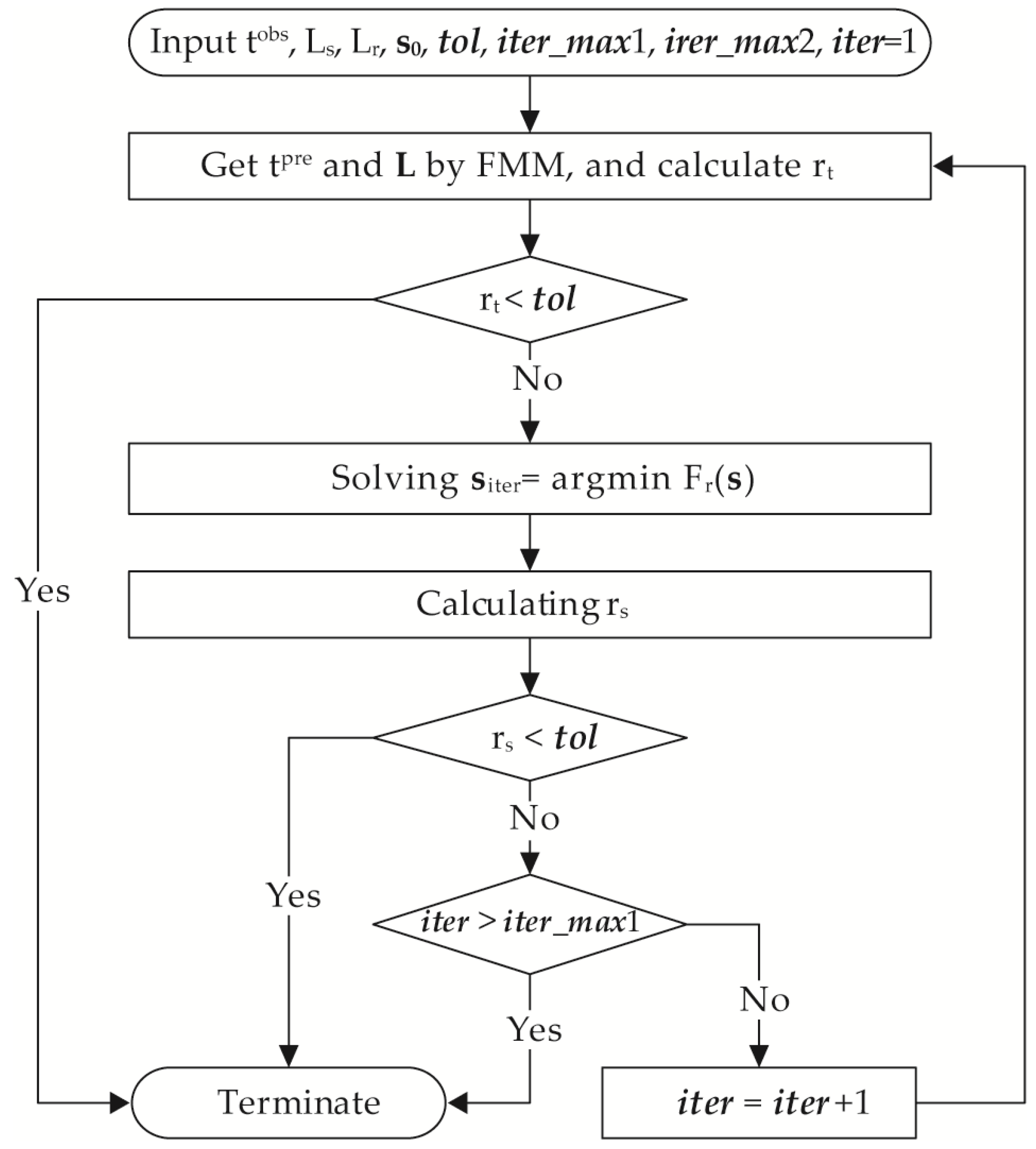
To obtain a more accurate velocity distribution, an iterated inversion process was necessary. The ray-tracing tomographic inversion algorithm we used included following steps:

• Input observed data ($t^{\mathrm{obs}}$) and the positions of the sources (L_s) and receivers (L_r) and make an initial guess for the slowness ($s_0$). Set the tolerance (tol), maximum iteration numbers (iter_max1) of ray-tracing, maximum iteration numbers (iter_max2) of regularization inversion, and the initial counter of iteration (iter) to 1.
• Calculate predicted travel time ($t^{\mathrm{pre}}$) and construct the L Matrix by FMM for the initial velocity or updated velocity model.
• Calculate the root-mean-square (RMS, Equation (7)) value $r_t$ of $\mathsf{\delta }t=t^{\mathrm{pre}}-t^{\mathrm{obs}}$. If $r_t$ is less than tol, terminate, else, go to next step:

  $$\mathrm{RMS}=\sqrt{{\displaystyle \sum _{n=1}^N{(\delta t_n^{})}^2}/\mathrm{N}}.$$

  (7)
• Solve the regularization problem $s_{iter}=\arg \min {\mathrm{F}}_{\mathrm{r}}(\mathrm{s})$.
• Calculate the RMS value $r_s$ of $s_{iter}-s_{iter-1}$. If $r_s$ is less than tol, stop, else, go to next step.
• Set iter = iter + 1. If iter > iter_max1, stop, else, go to step 2.
• Terminate.

The procedures above can also be seen in Figure 1.

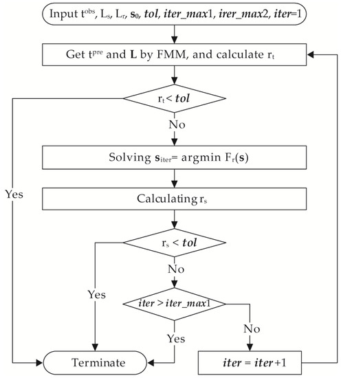
Figure 1. The flow chart of the ray-tracing tomographic inversion algorithm.

3. Numerical Simulation

3.1. Constructing a Velocity Model

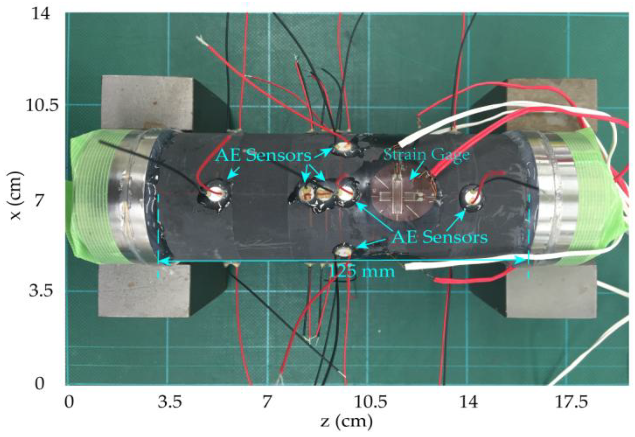
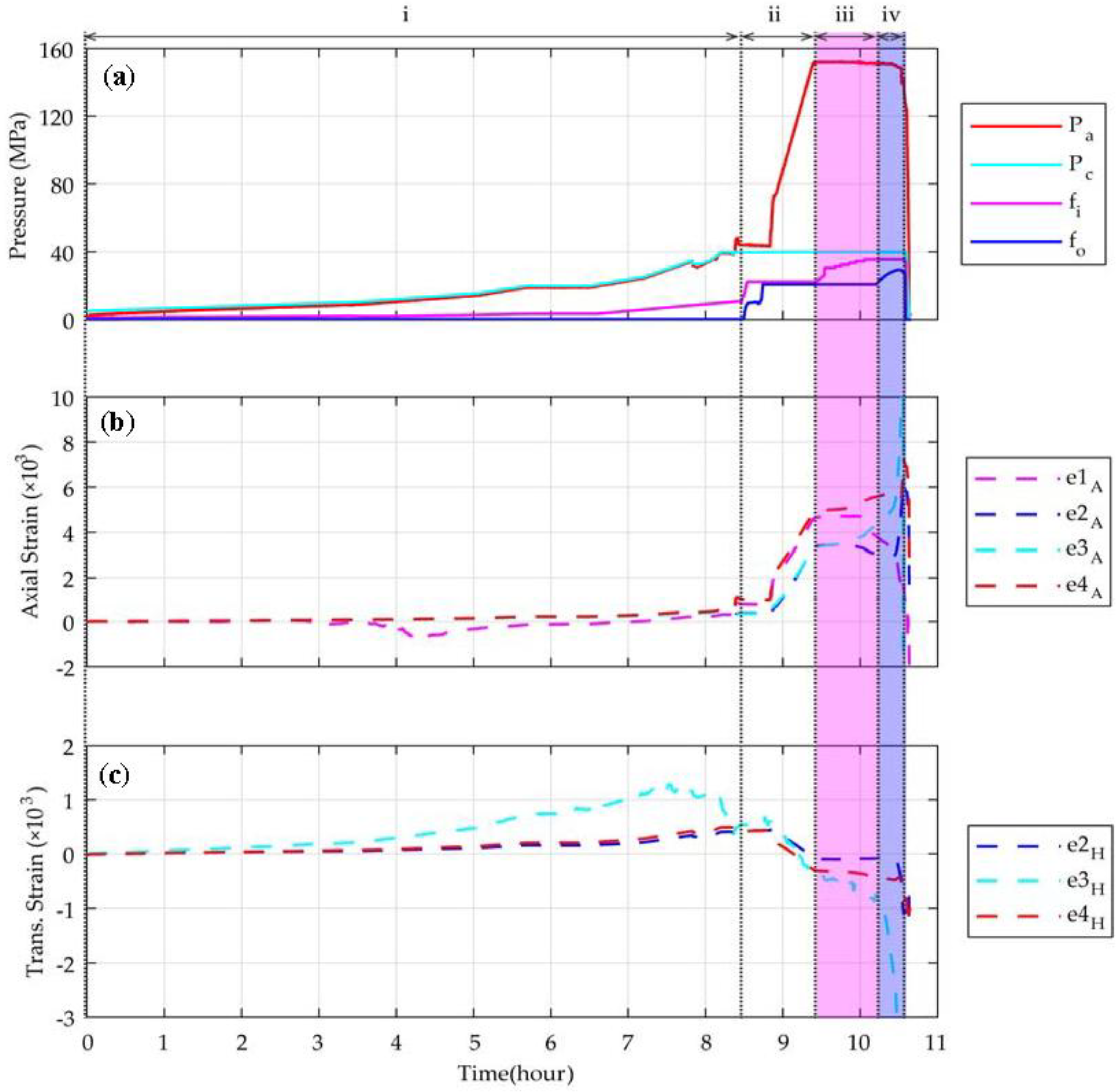
We conducted a hydraulic fracturing experiment on a shale column (length of 125 mm and radius of 25 mm, Figure 2) from the Lower Silurian Longmaxi formation in the Sichuan basin, China. The experiment was mainly divided into four stages (Figure 3): (i) the gradual increase of the axial and confining pressure, and the closure of the natural fractures; (ii) water injection and the dilatancy of the sample; (iii) hydraulic fracturing process and the further expansion of the pre-existing fracture; (iv) breakthrough of the water from the inlet side and rapidly fracturing process (the further details of this experiment has been illustrated in [26]).

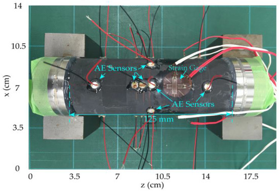
Figure 2. The shale column with the AE sensors and strain gauge installed on it.

Figure 3. Stress loading and water injection processes for the sample, and the plots of strain curves. (a) numbers i–iv indicate loading and injection stages. P_a and P_c represent axial stress and confining pressure, respectively. f_i and f_o represent injection pressure from pump A and pump B, respectively; (b) axial strains monitored by sensor e1–e4; (c) circumferential strains monitored by sensors e2–e4, and the e1_H was broken or shorted before the test. (Figure 5 in [26]).

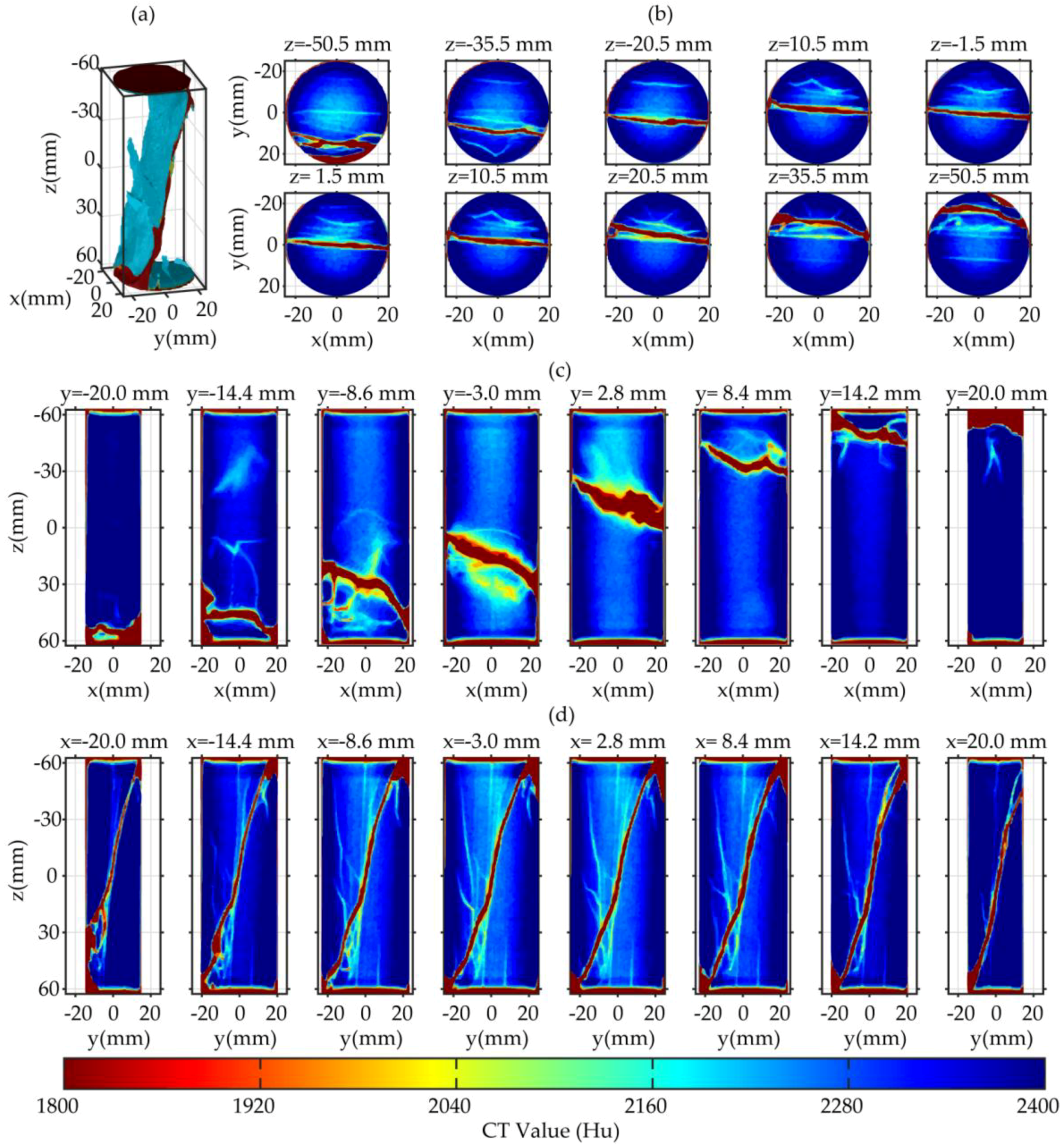
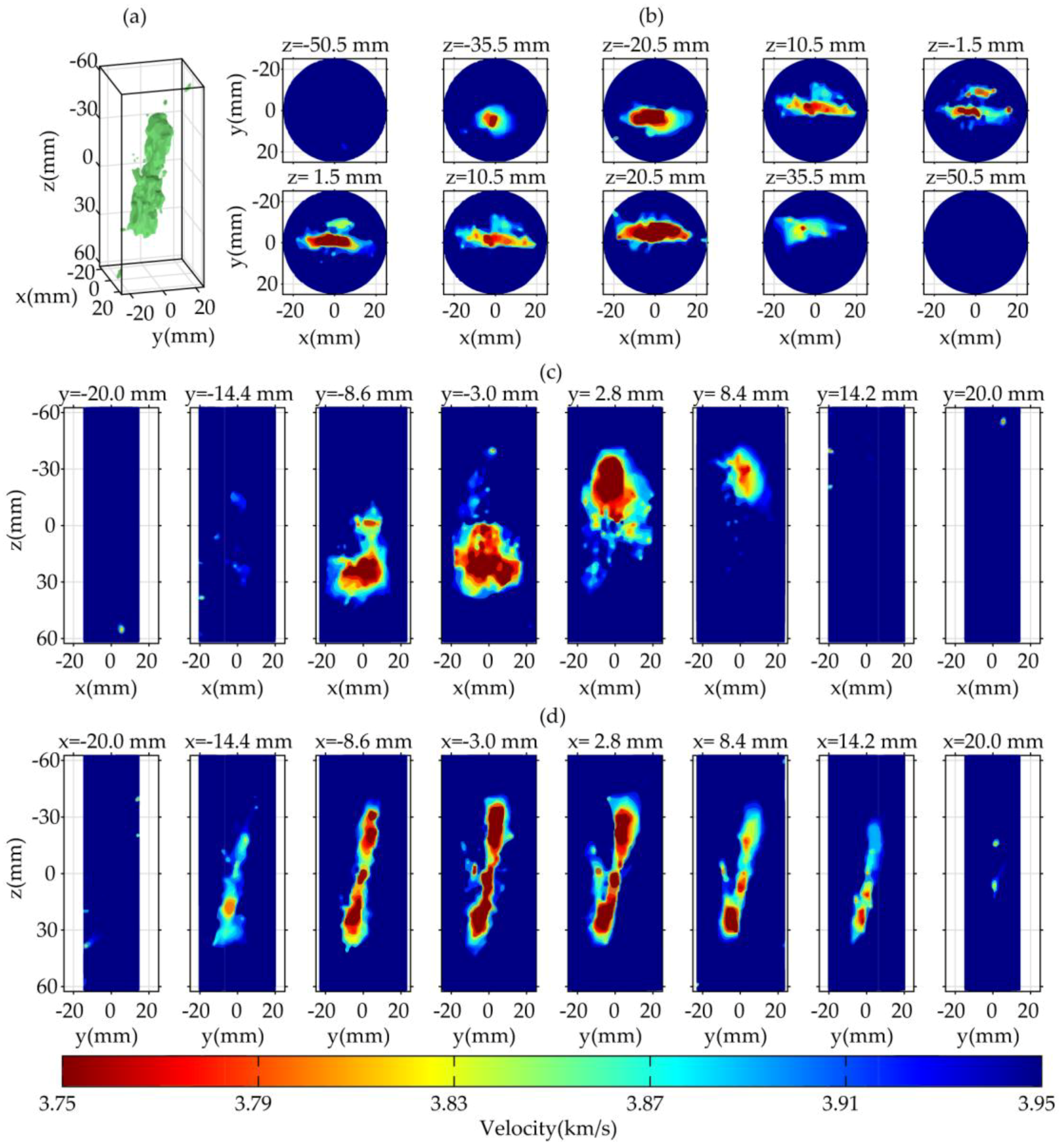
After the experiment, we got a 3D image (Figure 4) of the hydraulic fractures in the column using a medical X-CT scanning equipment (Aquilion ONE TSX 301A, Toshiba Medical Systems Corp., Kyoto, Japan, belonging to the Research Institute of Innovative Technology for the Earth, the parameter settings are listed in Table 1). The 3D X-CT image has voxel dimensions of 0.108 mm × 0.108 mm × 0.50 mm. As is shown in Figure 4, there is one fat primary fracture and multiple thin secondary fractures in the shale column.

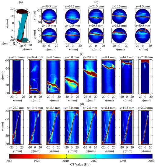
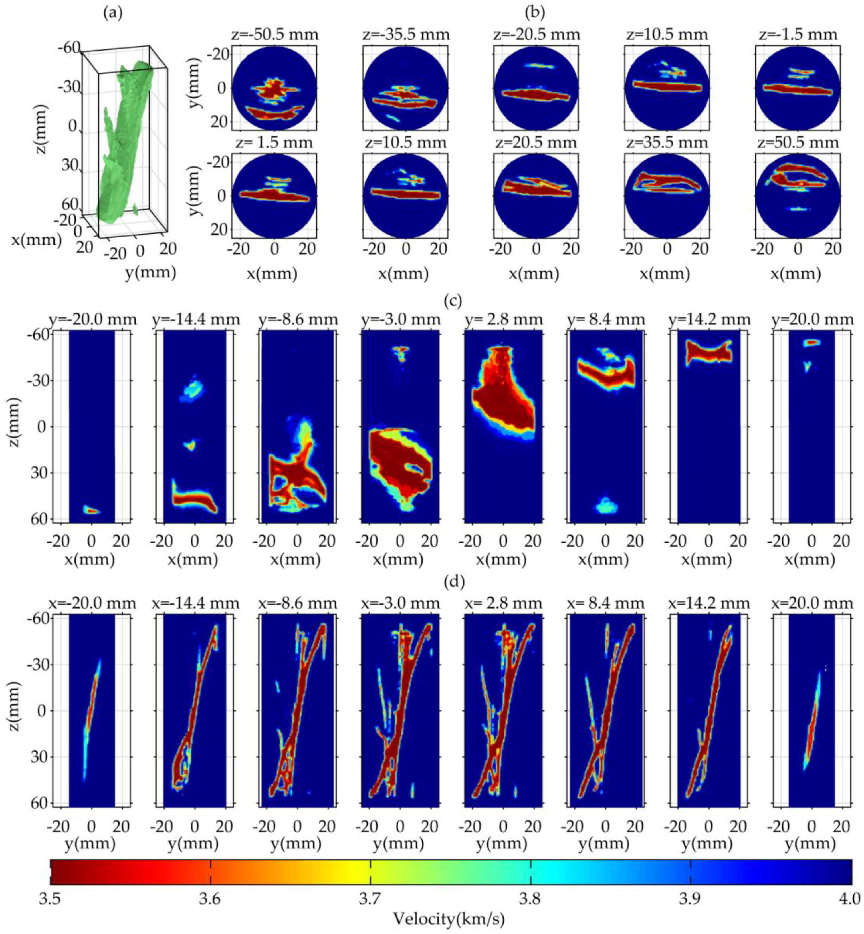
Figure 4. The X-CT scanning image for a hydraulic fractured shale column. (a) the 3D segmented image; (b) the transverse-view profile; (c) the coronal-view profile; (d) the sagittal-view profile. The caption of each sub-image in (b–d) represents the profile position.

Table 1. The parameter settings for the X-CT scanning equipment.

Voltage	Current	Slice Thickness	Pixel Spacing	Pixel Matrix Size
135 kV	150 mA	0.5 mm	0.108 mm	512 pixels × 512 pixels

We assumed that the velocity distribution is consistent with the CT value distribution. Then, we constructed a velocity model with fractures based on the 3D distribution of the CT value (Figure 5). By analyzing the distribution of the CT value, we found that it is mainly distributed in 2200–2600 Hu. To simplify the model, we firstly converted X-CT photos into a binary one at the boundary of 2200 Hu, and then we again discretized the image in a new cell dimension corresponding to the ultrasonic wavelength. The optimal cell dimension can be determined by Equations (8) and (9):

$${\lambda }_{\min }=v_{\min }/f_{\max },$$

(8)

$$\max \{\Delta x,\Delta y,\Delta z\}=0.5{\lambda }_{\min },$$

(9)

where v_min is the minimum velocity and f_max is the dominant frequency of the ultrasound [27]. Meanwhile, according to [15], the corner frequency of laboratory AE is around 1 MHz when the fracture dimension is 1 mm. Because of this, the dominant frequency can be set to 1.5 MHz. In this case, the optimal cell dimension is 1.17 mm. However, the number of the cells must be an integer, so we adopted an approximate value, i.e., 1 mm. Thus, in this study, the UTT has voxel dimensions of 1 mm × 1 mm × 1 mm for the dominant frequency of 1.5 MHz. After discretization, we need to choose an appropriate velocity contrast. When passive sources occur, the sample is still stressed, and the fractures are not fully open; due to this, the velocity contrast is not very high. Thus, we set background velocity of the model to 4 km/s, and the velocity in the crack to 3.5 km/s. Figure 6 displays the velocity model we constructed. It is evident that this model preserves the main structure and several thin fractures of the X-CT image.

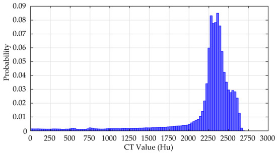
Figure 5. The CT value distribution histogram of hydraulically fractured shale column.

Figure 6. The velocity model. (a) the 3D segmented image; (b) the transverse-view profile; (c) the coronal-view profile; and (d) the sagittal-view profile. The caption of each sub-image in (b–d) represents the profile position.

3.2. Observation Geometry

To verify the feasibility, the effectiveness, and the accuracy of inversion algorithm, we performed tomographic inversion under dense and sparse ray coverage. For the dense case, there were 285 sources set in the column based on real acoustic emission location results, and there were 130 receivers placed around the model (Figure 7). However, the receiver configuration in the dense case is nearly impossible for the real experiment. In the hydraulic fracturing experiment, we used piezoelectric sensors with a diameter of 5 mm (Figure 2) as the AE sensors. According to this, we arranged 35 receivers around the model. To further reduce the ray-coverage, we randomly choose 95 sources of the 285 sources. That is to say, in the sparse ray-coverage case, there are only 35 receivers, and 95 sources are placed (Figure 8).

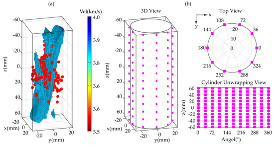
Figure 7. (a) 285 sources (red dot) set in the rock column; (b) 130 receivers (magenta square) placed around it under dense ray-coverage case and the observation geometry is shown in three views.

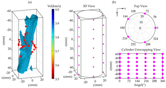
Figure 8. (a) 95 sources (red dot) set in the rock column; (b) 35 receivers (magenta square) placed around it under dense ray-coverage case and the observation geometry is shown with three views.

3.3. Simulated Observed Travel-Time

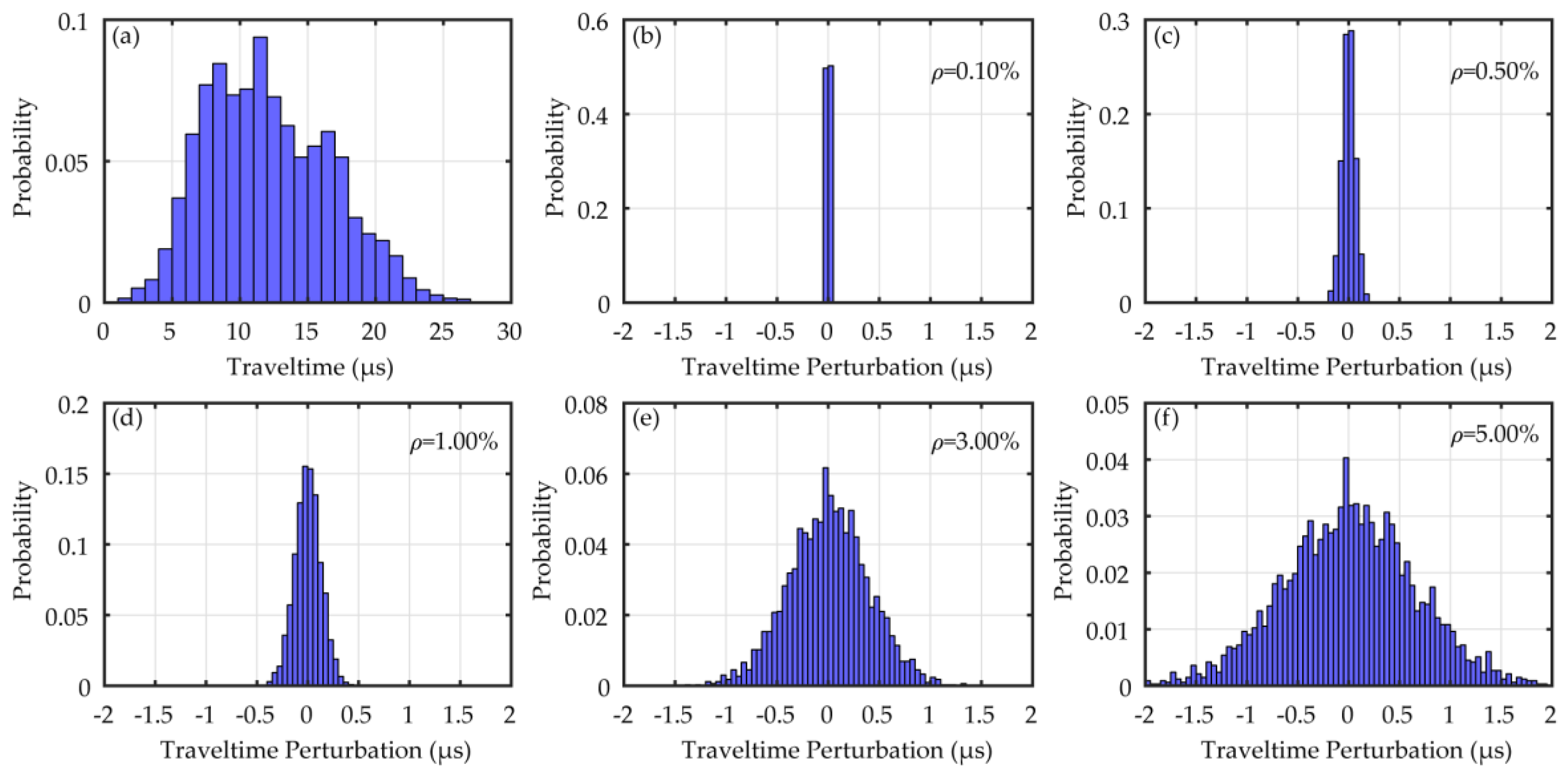
We utilized the fast-marching method to calculate ray-paths and travel-times corresponding to the different source–receiver configuration and got five simulated observed travel-times using Equation (3) with RNL equaling to 0.1%, 0.5%, 1%, 3%, and 5%. Figure 6 shows the histogram of the calculated travel-time $t^{\mathrm{cal}}$ and the corresponding travel-time perturbation. From Figure 9, we can see that the travel-time perturbation nearly is the minimum value of the $t^{\mathrm{cal}}$ when RNL is 3% and 5%, and it is a great challenge for velocity reconstruction using regularization.

Figure 9. (a) the histogram of travel time calculated by FMM; (b–f) the histograms of the perturbation for 0.1%, 0.5%, 1%, 3%, and 5% noised travel time.

4. Results and Discussion

4.1. Tomographic Images

To illustrate the superiority of TVR under sparse ray-coverage, we provided the pictures inversed with data under dense ray-coverage. Meanwhile, to compare with the inversion methods limited by Nyquist, we also gave the inversion results solved with Tikh under both dense and sparse cases. To enhance the contrast, all the tomographic images in this section are shown with a velocity range of 3.75–3.95 km/s.

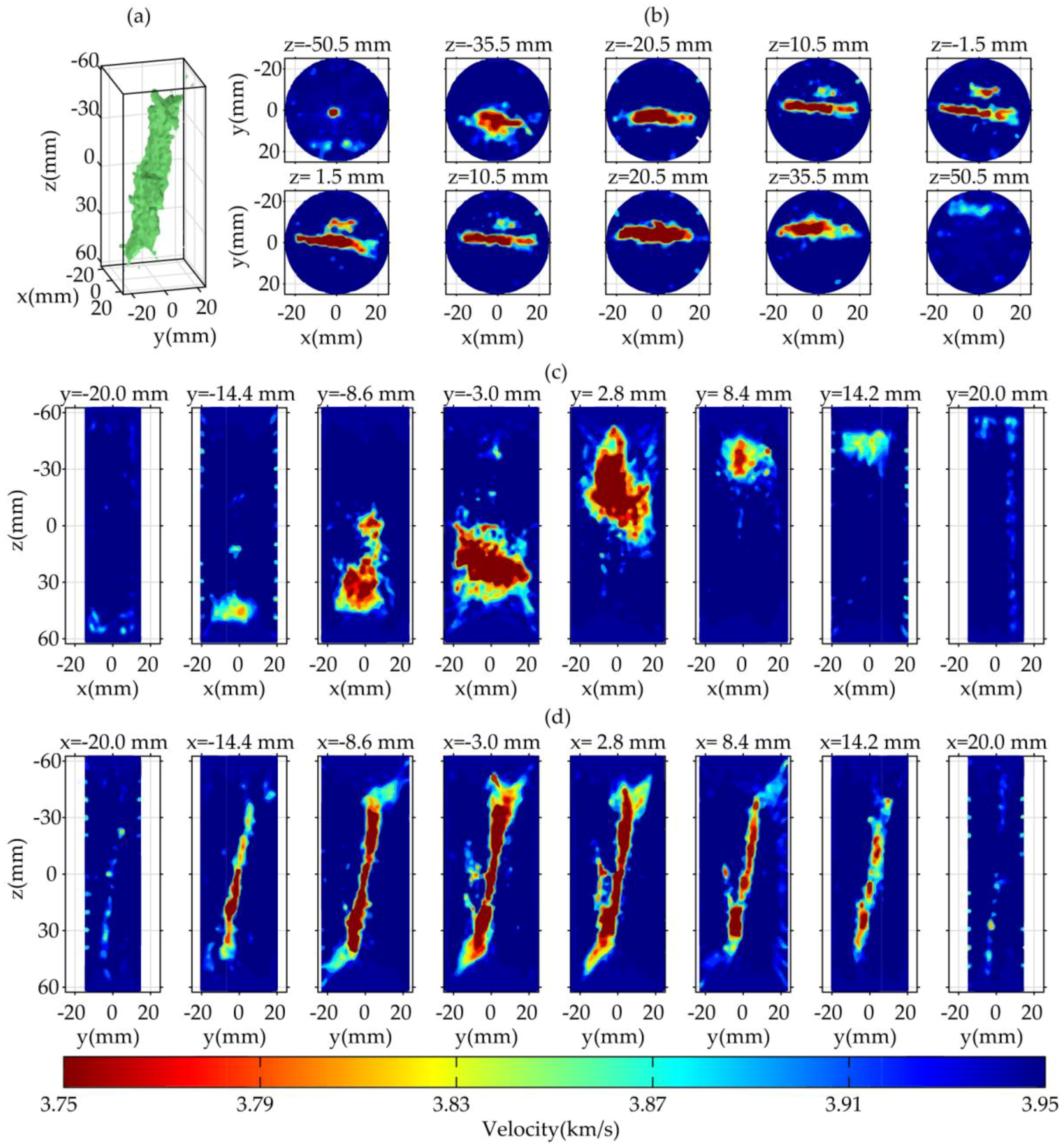
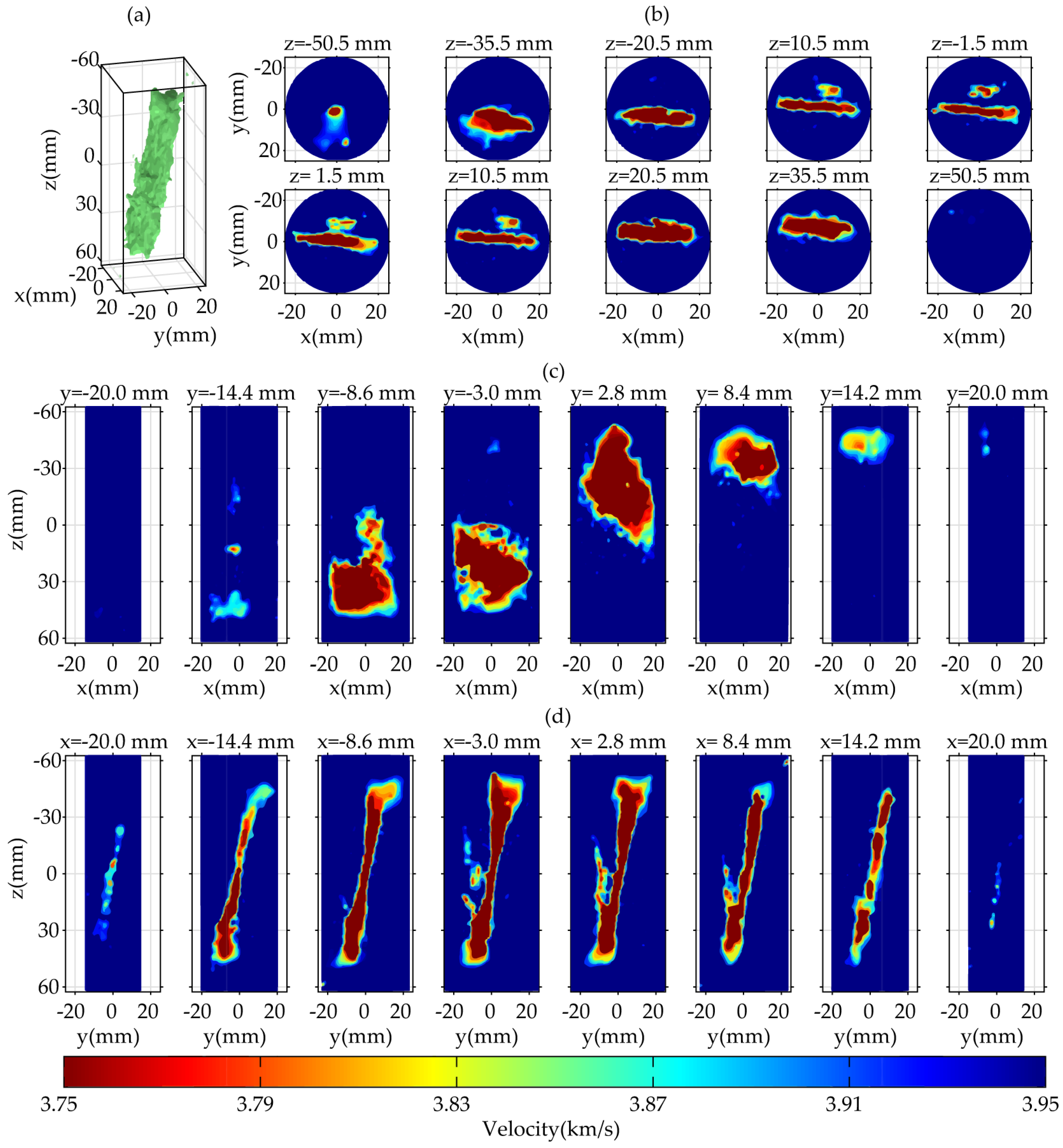
Figure 10 and Figure 11 show resulting tomographic photos solved respectively with Tikhonov and total variation regularization under dense ray-coverage with correct travel time. As can be seen from these two figures, both Tikh and TVR can reasonably characterize the major features and a few details of the fractures with sufficient data. However, in the images solved by Tikh, there exist too many unwanted artifacts for us to interpret them as fractures or not. Conversely, TVR gives sharper edges of the fractures and smoother background velocity, which is very helpful to depict the fractures correctly. Notwithstanding, when compared with the real velocity model and X-CT images, the fractures are not adequately described neither by Tikh nor TVR, especially in the regions of low coverage. Given this, we must be cautious when interpreting the UTT images in these regions.

Figure 10. Tomographic images of Tikh in dense ray coverage case. (a) the 3D segmented image; (b) the transverse-view profile; (c) the coronal-view profile; and (d) the sagittal-view profile. The caption of each sub-image in (b–d) represents the profile position.

Figure 11. Tomographic images of TVR under dense ray-coverage case. (a) the 3D segmented image; (b) the transverse-view profile; (c) the coronal-view profile; and (d) the sagittal-view profile. The caption of each sub-image in (b–d) represents the profile position.

Similarly, Figure 12 and Figure 13 display tomographic images inversed with Tikh and TVR, respectively, under sparse ray-coverage with observed travel-time without noising. Naturally, both the resolution of the tomographic images solved by these two methods decrease significantly due to the reduction of the observed data. By comparing the two results, it can be seen that TVR can still more clearly outline the fracture geometry than Tikh. Moreover, the thin cracks can also be delineated, though they cannot be seen as clearly as the dense case. Therefore, when we characterize the fracture morphology with these images in the sparse case, we must know explicitly where the believable or receivable regions are in the inversion results.

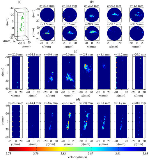
Figure 12. Tomographic images of Tikh under sparse ray coverage case. (a) the 3D segmented image; (b) the transverse-view profile; (c) the coronal-view profile; and (d) the sagittal-view profile. The caption of each sub-image in (b–d) represents the profile position.

Figure 13. Tomographic images of TVR under sparse ray-coverage. (a) the 3D segmented image; (b) the transverse-view profile; (c) the coronal-view profile; and (d) the sagittal-view profile. The caption of each sub-image in (b–d) represents the profile position.

Additionally, we also give the inversion results solved from the noised travel time in the Supplementary Materials under the sparse ray-coverage case. According to these results, we can see that both the tomographic pictures solved by these two methods have almost the same resolution as the results solved with correct travel time, when RNL is 0.1%, 0.5%, and 1%. However, both the resolution of the results solved by Tikh and TVR dramatically decreased, and the fractures’ geometry is also heavily distorted when RNL is 3% and 5%. Interestingly, we can still identify the primary geometry of the fractures from the results solved by TVR, even with a high RNL, such as 3%, but the results solved by Tikh cannot. That is to say, the TVR is more stable and credible than Tikh. Even so, we must pay more attention to the artifacts and distortion caused by the noise when describing the geometry of fractures.

Overall, these results suggest that both Tikh and TVR can reasonably describe the primary features of the real velocity model, but TVR delineates more and better details and sharper edges of the mode. This superiority is especially prominent in the sparse case. Apparently, the total variation regularization is more effective and precise than Tikhonov regularization. The results solved with the noised travel time also verify that TVR has better stability than Tikh. Moreover, it is necessary to consider the influence of the nonuniform ray-coverage and noise when we interpret the inversion pictures.

4.2. Errors Analysis

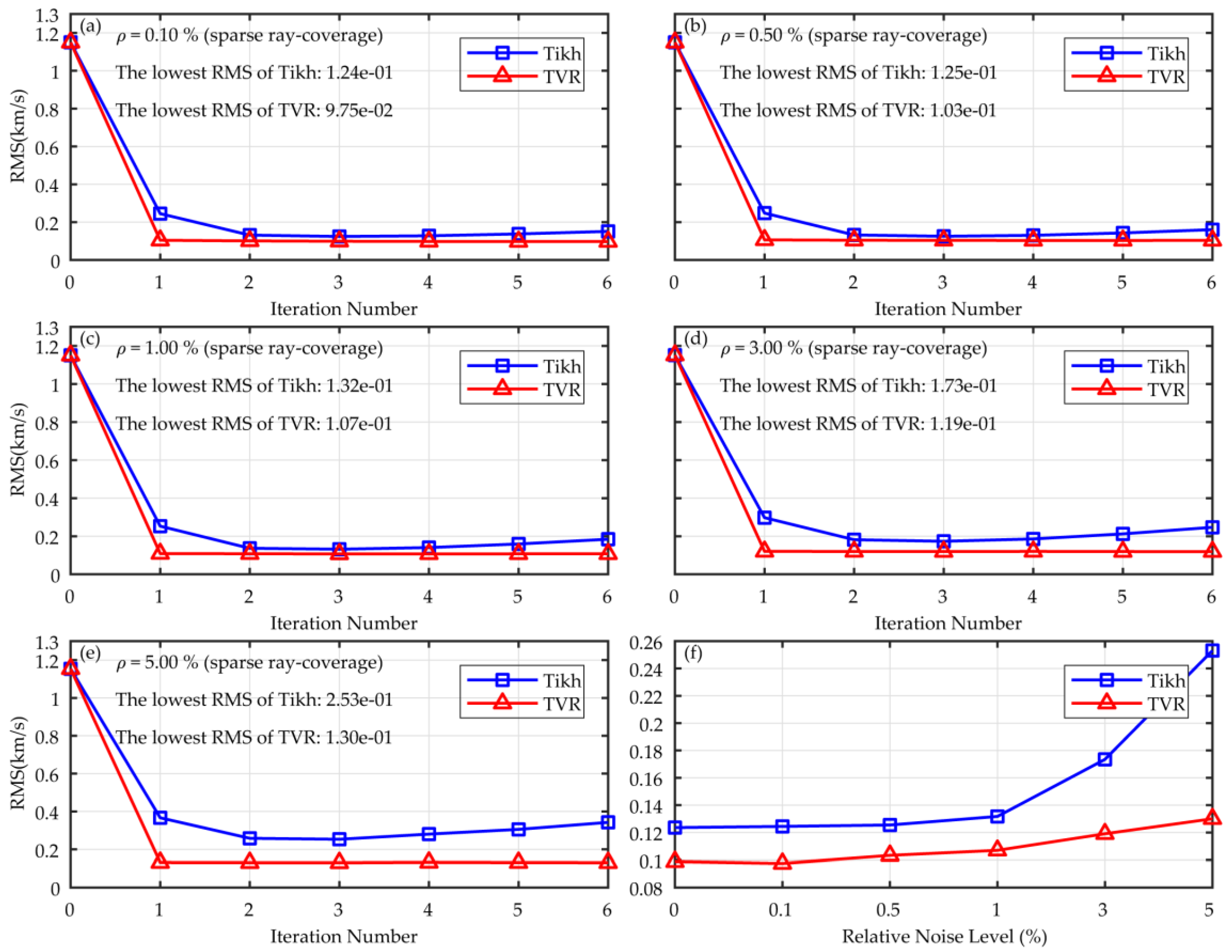
To verify the confidence of the tomographic inversions, RMS errors between inversion results and the real model were calculated for the simulated observed travel time at every iteration (Figure 14 and Figure 15). As shown in Figure 14, TVR has a faster convergence and lower RMS errors under both the dense and sparse case. However, for Tikh, RMS errors decrease until the third iteration, and then it starts increasing again in the case of sparse ray-coverage. In contrast, for TVR, this never occurs during the six iterations. The same case also happens for the inversion results solved from noised travel time with different RNL (Figure 15). Besides, we also find that both the RMS errors of Tikh and TVR increase with the rising of RNL according to Figure 15f. What is striking in this graph is that the growth trend is not linear but initially increases slowly then sharply; this phenomenon suggests that both Tikh and TVR have excellent noise tolerance at low RNL, but TVR does better at the high RNL.

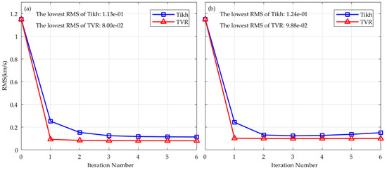
Figure 14. The convergence curve of RMS for velocity solved with correct t^cal. (a) the dense ray-coverage case; and (b) the sparse ray-coverage case. The blue points are the results solved with Tikh, and the red points are the results solved with TVR. The lowest RMS of the results solved by these two methods are both marked in the graph.

Figure 15. (a–e) the convergence curve of RMS for velocity solved with noised T under the sparse ray-coverage case. The RNL of (a–e) respectively is 0.1%, 0.5%, 1.0%, 3.0%, 5.0%; (f) the comparison of RMS of velocity among the inversion results under different relative noise level. The blue points are the results solved with Tikh, and the red points are the results solved with TVR. The RNL and lowest RMS of the results solved by the Tikh and TVR are marked on (a–e).

All of this illustrates that TVR is more stable than Tikh. Moreover, the RMS errors of TVR between the resulting tomographic inversions and the real model are always lower than those of the Tikh under the different RNL. Hence, we can undeniably say that the total variation regularization is more accurate and reliable than the Tikhonov regularization.

4.3. Comparison with the X-CT

To illustrate the success of the UTT, we introduce the Structural Similarity Index (SSIM) [28] to evaluate the similarity between UTT image and X-CT image. The bigger the SSIM, the more similar the two images are. Suppose X and Y are two images; SSIM is defined as below:

$$\mathrm{SSIM}=\frac{(2{\mu }_1{\mu }_2+C_1)(2{\sigma }_{12}+C_2)}{({\mu }_1^2+{\mu }_2^2+C_1)({\sigma }_1^2+{\sigma }_2^2+C_2)},$$

where ${\mu }_1$, ${\mu }_2$ is respectively the mean intensity of X and Y, and ${\sigma }_1$, ${\sigma }_2$ is respectively the standard deviation of X and Y, and ${\sigma }_{12}$ is defined as

$${\sigma }_{12}=\frac{1}{N-1}{\displaystyle \sum _{i=1}^N({\mathrm{X}}_i-{\mu }_1)({\mathrm{Y}}_i-{\mu }_2)},$$

where N is the total voxel number, ${\mathrm{X}}_i$ and ${\mathrm{Y}}_i$ are respectively image intensity in the ith voxel.

To eliminate the effect of index dimension and quantity of UTT and X-CT, we respectively convert UTT and X-CT to the grayscale image. We calculate the SSIM between UTT grayscale images and X-CT grayscale images (Table 2). Due to the lower ray-coverage out of the range −40~40 mm, the inversed results in these regions are not reliable. Thus, we neglect these values when calculating the SSIM. As a comparison, the SSIM of a real velocity model compared with X-CT is also given. The SSIM of real model grayscale images is 0.2035 compared with X-CT grayscale images. Although this value is not very high, the UTT is successful in comparison to X-CT measurements, as long as the SSIM of inversion results is close to it. From Table 2, we can see that TVR has a closer SSIM to the real model than Tikh for the dense case, sparse case, and noised case. This illustrates that the inversion results solved with TVR are more similar with X-CT than Tikh. Meanwhile, we can also find that the SSIM of TVR approximate 0.2035 when RNL < 1, which suggests that TVR is a stable method.

Table 2. SSIM of UTT grayscale images compared with X-CT grayscale images.

RNL(%)	SSIMt	SSIMtv
0 (dense case)	0.1524	0.1878
0 (sparse case)	0.1269	0.1663
0.1	0.1263	0.1704
0.5	0.1268	0.1574
1	0.1211	0.1498
3	0.0985	0.1287
5	0.0904	0.1183

SSIM_t, and SSIM_tv are respectively referred to the SSIM of grayscale images for real model, Tikh, and TVR compared with the X-CT image. The SSIM of real model grayscale images is 0.2035.

5. Conclusions

The application of acoustic emission ultrasonic 3D tomography in imaging the cracks of hydraulically fractured shale is investigated and the main procedures of tomographic ray-tracing iteration inversion algorithm are given. Results show that TV regularization can reasonably characterize and reveal the fractures geometry both in the case of dense and sparse ray-coverage, and it is stable and robust in the case of a high noise level. Due to the non-uniform ray-coverage, TVR cannot perfectly reconstruct the fracture morphology, but we could still build a pretty good understanding of these as long as a rational interpretation method is built. Additionally, by computing the SSIM of UTT grayscale images compared with X-CT, the inversion results solved with TVR are quite close to the SSIM of the real model. Thus, with regards to understanding the fracture process, it can be a valid alternative for X-CT.

AE sources ultrasonic travel-time tomography based on TV regularization can accurately, efficiently, and stably reconstruct the velocity structures with fractures. X-CT can be partly replaced with it to reconstruct the hydraulic fractures via a proper interpretation.

References

- Chitrala, Y.; Moreno, C.; Sondergeld, C.H.; Rai, C.S. Microseismic Mapping of Laboratory Induced Hydraulic Fractures in Anisotropic Reservoirs. In Proceedings of the SPE Tight Gas Completions Conference, San Antonio, TX, USA, 2–3 November 2010. [Google Scholar]
- Benson, P.M.; Thompson, B.D.; Meredith, P.G.; Vinciguerra, S.; Young, R.P. Imaging slow failure in triaxially deformed Etna basalt using 3D acoustic-emission location and X-ray computed tomography. Geophys. Res. Lett. 2007, 34. [Google Scholar] [CrossRef]
- Krilov, Z.; Goricnik, B. SPE 36879 A Study of Hydraulic Fracture Orientation by X-ray Computed Tomography. In Proceedings of the SPE European Petroleum Conference, Milan, Italy, 22–24 October 1996. [Google Scholar]
- Martínez-Martínez, J.; Fusi, N.; Galiana-Merino, J.J.; Benavente, D.; Crosta, G.B. Ultrasonic and X-ray computed tomography characterization of progressive fracture damage in low-porous carbonate rocks. Eng. Geol. 2016, 200, 47–57. [Google Scholar] [CrossRef]
- Otani, J.; Mukunoki, T.; Obara, Y. Application of X-ray CT method for characterization of failure in soils. Soils Found. Jpn. Geotech. Soc. 2000, 40, 111–118. [Google Scholar] [CrossRef]
- Falls, S.D.; Young, R.P.; Carlson, S.R.; Chow, T. Ultrasonic tomography and acoustic emission in hydraulically fractured Lac du Bonnet Grey granite. J. Geophys. Res. 1992, 97, 6867–6884. [Google Scholar] [CrossRef]
- Mitra, R. Imaging of Stress in Rock Samples Using Numerical Modeling and Laboratory Tomography. Ph.D. Thesis, Virginia Polytechnic Institute and State University, Blacksburg, VA, USA, 2006. [Google Scholar]
- Charalampidou, E.-M. Experimental Study of Localised Deformation in Porous Sandstones. Ph.D. Thesis, Heriot Watt University, Edinburg, UK, 2011. [Google Scholar]
- Tudisco, E. Development and Application of Time-Lapse Ultrasonic Tomography for Laboratory Characterisation of Localised Deformation in Hard Soils/Soft Rocks. In Proceedings of the 16th International Conference on Experimental Mechanics, Lund University, Lund, Sweden, 7–11 July 2014. [Google Scholar]
- Lei, X.; Xue, Z. Ultrasonic velocity and attenuation during CO2 injection into water-saturated porous sandstone: Measurements using difference seismic tomography. Phys. Earth Planet. Inter. 2009, 176, 224–234. [Google Scholar] [CrossRef]
- Shiotani, T.; Osawa, S.; Kobayashi, Y. Application of 3D AE Tomography for Triaxial Tests of Rocky Specimens. In Proceedings of the European Working Group on Acoustic Emission, Dresden, Germany, 3–5 September 2014; pp. 1–9. [Google Scholar]
- Yang, T.; Westman, E.C.; Slaker, B.; Ma, X.; Hyder, Z.; Nie, B. Passive tomography to image stress redistribution prior to failure on granite. Int. J. Min. Reclam. Environ. 2015, 29, 178–190. [Google Scholar] [CrossRef]
- Jerri, A.J. The Shannon Sampling Theorem—Its Various Extensions and Applications: A Tutorial Review. Proc. IEEE 1977, 65, 1565–1596. [Google Scholar] [CrossRef]
- Daigle, M.; Fratta, D.; Wang, L.B. Ultrasonic and X-ray Tomographic Imaging of Highly Contrasting Inclusions in Concrete Specimens. In Proceedings of the GeoFrontier 2005 Conference, Austin, TX, USA, 24–26 July 2005; pp. 1–12. [Google Scholar]
- Lei, X.; Ma, S. Laboratory acoustic emission study for earthquake generation process. Earthq. Sci. 2014, 27, 627–646. [Google Scholar] [CrossRef]
- Lin, Y.; Syracuse, E.M.; Maceira, M.; Zhang, H.; Larmat, C. Double-difference traveltime tomography with edge-preserving regularization and a priori interfaces. Geophys. J. Int. 2015, 201, 574–594. [Google Scholar] [CrossRef]
- Tikhonov, A.N.; Arsenin, V.Y. Solutions of Ill-Posed Problems; Fritz Jhon, Ed.; John Wiley and Sons, Inc.: Hoboken, NJ, USA, 1977. [Google Scholar]
- Donoho, D.L. Compressed Sensing. IEEE Trans. Inf. Theory 2006, 52, 1289–1306. [Google Scholar] [CrossRef]
- Lin, Y.; Huang, L.; Zhang, Z. Ultrasound waveform tomography with the total-variation regularization for detection of small breast tumors. In Proceedings of the SPIE, San Diego, CA, USA, 24 February 2012. [Google Scholar]
- Jiang, W.; Zhang, J. First-arrival traveltime tomography with modified total-variation regularization. Geophys. Prospect. 2017, 65, 1138–1154. [Google Scholar] [CrossRef]
- Zhang, X.; Zhang, J. Model regularization for seismic traveltime tomography with an edge-preserving smoothing operator. J. Appl. Geophys. 2017, 138, 143–153. [Google Scholar] [CrossRef]
- Neumann-Denzau, G.; Behrens, J. Inversion of seismic data using tomographical reconstruction techniques for investigations of laterally inhomogeneous media. Geophys. J. Int. 1984, 79, 305–315. [Google Scholar] [CrossRef]
- Sethian, J.A. Fast Marching Methods. SIAM Rev. 1999, 41, 199–235. [Google Scholar] [CrossRef]
- Jensen, T.L.; Jørgensen, J.H.; Hansen, P.C.; Jensen, S.H. Implementation of an optimal first-order method for strongly convex total variation regularization. BIT Numer. Math. 2012, 52, 329–356. [Google Scholar] [CrossRef]
- Hansen, P.C.; O’Leary, D.P. The use of the L-curve in the regularization of discrete ill-posed problems. SIAM J. Sci. Comput. 1993, 14, 1487–1503. [Google Scholar] [CrossRef]
- Zhai, H.; Chang, X.; Wang, Y.; Xue, Z.; Lei, X.; Zhang, Y. Sensitivity analysis of seismic velocity and attenuation variations for longmaxi shale during hydraulic fracturing testing in laboratory. Energies 2017, 10, 1393. [Google Scholar] [CrossRef]
- Martins, J.L.; Soares, J.A.; Silva, J.C. Da Ultrasonic travel-time tomography in core plugs. J. Geophys. Eng. 2007, 4, 117–127. [Google Scholar] [CrossRef]
- Wang, Z.; Bovik, A.C.; Sheikh, H.R.; Simoncelli, E.P. Image quality assessment: From error visibility to structural similarity. IEEE Trans. Image Process. 2004, 13, 600–612. [Google Scholar] [CrossRef] [PubMed]
© 2018 by the authors. Licensee MDPI, Basel, Switzerland. This article is an open access article distributed under the terms and conditions of the Creative Commons Attribution (CC BY) license (http://creativecommons.org/licenses/by/4.0/).