A Prediction Mechanism of Energy Consumption in Residential Buildings Using Hidden Markov Model

Abstract

Internet of Things (IoT) is considered as one of the future disruptive technologies, which has the potential to bring positive change in human lifestyle and uplift living standards. Many IoT-based applications have been designed in various fields, e.g., security, health, education, manufacturing, transportation, etc. IoT has transformed conventional homes into Smart homes. By attaching small IoT devices to various appliances, we cannot only monitor but also control indoor environment as per user demand. Intelligent IoT devices can also be used for optimal energy utilization by operating the associated equipment only when it is needed. In this paper, we have proposed a Hidden Markov Model based algorithm to predict energy consumption in Korean residential buildings using data collected through smart meters. We have used energy consumption data collected from four multi-storied buildings located in Seoul, South Korea for model validation and results analysis. Proposed model prediction results are compared with three well-known prediction algorithms i.e., Support Vector Machine (SVM), Artificial Neural Network (ANN) and Classification and Regression Trees (CART). Comparative analysis shows that our proposed model achieves $2.96\%$ better than ANN results in terms of root mean square error metric, $6.09\%$ better than SVM and $9.03\%$ better than CART results. To further establish and validate prediction results of our proposed model, we have performed temporal granularity analysis. For this purpose, we have evaluated our proposed model for hourly, daily and weekly data aggregation. Prediction accuracy in terms of root mean square error metric for hourly, daily and weekly data is 2.62, 1.54 and 0.46, respectively. This shows that our model prediction accuracy improves for coarse grain data. Higher prediction accuracy gives us confidence to further explore its application in building control systems for achieving better energy efficiency.

1. Introduction

Electrical energy is a very important but scarce resource available to humans. It has become an integral part of our lives and we cannot think of a world without electricity. Many household appliances are running on electricity and its demand is rapidly growing. Industries are also putting more pressure on electricity generating companies to produce more and more energy [1]. According to a report by US-Energy Information Administration (EIA), a $28\%$ increase in global energy demand is expected by 2040 [2]. To meet the rising worldwide demand for energy, efforts are made in two main directions: (a) increase electric power production capacity by exploiting existing and renewable energy sources and solutions (b) effectively utilize existing resources of energy by avoiding energy wastage and unnecessary usage. Both of these approaches are equally important and complement each other. In fact, the effective utilization of existing resources of energy is more desirable because it is economical and easy to adopt. Improper utilization of resources results in energy wastage which can otherwise be utilized in some useful application. To avoid wastage and unnecessary usage of energy, intelligent solutions are needed to ensure efficient utilization of energy.

Internet of Things (IoT)-based applications have shown promising results in many different fields by improving system efficiency, accuracy, process automation and overall profit maximization. IoT based technologies are also very useful in realizing the concept of smart homes. IoT devices are small devices attached to daily life objects for purpose of monitoring or controlling [3]. The devices have the capability of communication so that it can be accessed over the Internet. Integration of IoT with artificial intelligence algorithms provides the basic building blocks for the future smart world. To achieve energy efficiency in buildings, various IoT-based solutions can be found in the literature. According to a survey, energy efficiency and management are the second most promising domain for IoT applications in South Korea [4]. IoT devices have tiny sensors attached that can be used to gather sensing data about indoor building environment and appliances can intelligently be controlled according to user preferences [5]. Operating the electrical appliances only when required through IoT devices helps in avoiding energy wastage. However, any such solution for saving energy shall not have any negative impact on user comfort and convenience. In other words, the objective is to gain optimal utilization of energy without degrading user comfort.

Using IoT devices, we can collect desired context information about indoor environment including temperature, illumination, user occupancy, appliances operational status, etc. Various machine learning algorithms can be applied to collected context data to predict future conditions and corresponding energy requirement. Prediction energy requirement is both useful for home users and power generating companies. Home users can choose alternate strategies to reduce their energy expense e.g., automated switching from external power sources to an internal power source (e.g., solar system) when feasible. Furthermore, accurate estimation of future energy requirement can also help in identification and optimization of the peak hours for energy consumption. Better capacity planning can be done for managing on-site renewable energy generation and thus helpful in achieving the target of the zero-energy building. Similarly, energy prediction data can be used by power companies to timely adjust their generating capacity and optimize power load distribution. According to report by Korean Energy Economics Institute (KEEI) South Korea, $40\%$ of national energy consumption is covered by commercial and residential sector as shown in Figure 1 [6]. As electricity is contributing heavily to home user monthly expenses, therefore little achievement in optimal utilization of energy will cause a major reduction in overall expenses. Therefore, development of an intelligent IoT-based solution for achieving energy efficiency is highly desirable which is subject to this paper.

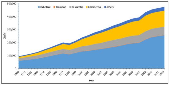
Figure 1. Annual energy consumption in various sectors, South Korea [6].

This paper is focused on the development of Hidden Markov Model (HMM) based algorithm to predict energy consumption in residential buildings. We have developed an HMM-based layered architecture for energy prediction in smart homes. The proposed architecture has four layers (a) Data acquisition layer is used to collect data including indoor environmental parameters, actuators status, and users occupancy information; (b) Pre-processing layer prepares the context data for upper layers; (c) Afterwards, hidden Markov models are generated and stored; (d) Finally, computed models are used at the application layer for energy prediction. For experimental analysis, we have used the data collected from four multi-storied buildings located in Seoul, South Korea. Comparative analysis shows that proposed model has achieved better results than Support Vector Machine (SVM), Artificial Neural Network (ANN) and Classification and Regression Trees (CART).

The rest of the paper is structured as follows. Section 2 present a brief overview on related work. A detailed discussion of hidden Markov modeling for proposed system is given Section 3 along with its pseudo code and flow diagram for HMM generation and training. The architecture of proposed HMM-based model for prediction of energy consumption is discussed in Section 4 along with its design. A brief discussion of collected data and its transformation is presented in Section 5. Section 6 presents model validation, comparative and temporal analysis along with a detailed discussion on results. Finally, the paper is concluded in Section 7 along with future work directions.

2. Related Work

Energy is considered as one of the most important and scarce resources due to the constant increase in its demand. Energy saving is not only desired for promoting a green environment for future sustainability but also important for the home users and energy production companies. Consumers want to reduce their monthly expenses in which electricity cost is a major contributor. Power generating companies are under pressure for producing more energy to fulfill commercial and domestic energy requirements. Thus, solutions for efficient energy utilization is desirable by all stock holders.

In the recent past, tremendous efforts have been invested in building smart homes solutions by researchers and manufacturing industry. In smart homes application domain, diverse nature of research directions can be found ranging from monitoring, prediction, optimization, security, privacy, and control. Energy optimization is also a profound area of research in building smart grids and smart homes. The objective is to provide maximum user comfort at the cost of minimum energy consumption [7,8,9].

Development of building energy management systems have been investigated based on various control systems [10,11,12]. Among the major reasons for energy inefficiencies and overutilization is that trivial systems often do not consider environmental factors and user occupancy. For instance, typical heating, ventilation, and air conditioning (HVAC) systems will assume that space is fully occupied and it will try to maintain the desired atmosphere without caring if a hall is fully occupied or only a few persons inside. Various algorithms are applied to predict user occupancy and corresponding energy requirement in order to improve system efficiency. Support vector machine and artificial neural networks-based algorithms are the two most widely used algorithms for energy prediction [13]. For instance, to improve the efficiency of a steam boiler in buildings, a data-driven scheme is proposed in [14] using artificial neural networks to achieve optimal cooling/heating. Their model can be used for estimation of steam consumption in future using forecasted weather data. Similarly, a model predictive control (MPC) based system is developed in [15] for saving of energy consumed by heating systems in buildings. Using forecasted weather data together with users occupancy information, the behavior of the building is modeled in terms of selected operational strategies. Their goal is to develop a control system that can achieve user desired parameters settings with minimum energy consumption. For indoor comfort and energy management, an intelligent multi-agent optimization based control system is presented in [16]. They try to achieve maximum user comfort with reduced energy consumption by fusing information using weighted aggregation.

Building energy management systems can be classified broadly into two categories based on adapted modeling strategies i.e., inverse and forward modeling [17]. A system based on an inverse modeling scheme tries to capture the dependencies among various inputs (e.g., users occupancy data, weather information, building structural parameters) and output data (i.e., required energy) in the form of a mathematical equation. However, this kind of system requires strong background knowledge to derive such a mathematical expression. In contrast, a system based on forward modeling schemes tries to generate an optimal schedule for operation along with estimated required energy by using input data such as building structural design parameters (e.g., size, material) along with weather and environmental information. Many software frameworks based on forward modeling schemes can be found in the literature. A comparative study of two of the most popular forward modeling-based software packages i.e., EnergyPlus and DOE-2 can be found in [18]. DOE-2 is famous simulation tool for energy usage estimation in residential and commercial buildings. Recent development in information and communication technologies (ICT) has given birth to new modeling schemes i.e., data-driven. Data-driven models are based on input data regarding outdoor and indoor environment collected through various sensors. In fact, this new sensor technologies-based data-driven approach is a hybrid model of both forward and inverse model for energy management. Forward models are based on input data which is supplied by various sensors readings. Inverse models are based on some mathematical relationship between inputs and outputs which can be derived by using various statistical or machine learning algorithms. A comprehensive review of data-driven approaches for prediction of energy consumption in buildings can be found in [19]. Since inception, sensing technologies-based models for energy management have attracted significant research attention. Several energy management systems are proposed in the literature for estimation and prediction of energy consumption by using hybrid models i.e., a combination of sensing technology with artificial intelligence algorithms. For instance, a study presented in [20] illustrate the application of several statistical methods in order to improve neural networks prediction for efficient energy consumption in buildings. Similarly, a hybrid model of adaptive-neuro-fuzzy system with genetic algorithm (GA-ANFIS) is presented in [21] for further improvement of conventional neural networks. Significant improvement in prediction results is reported by using the proposed hybrid model. Ali et al. proposed a hybrid energy prediction model to improve power consumption optimization based on pre and post processing in [22].

For required heating load prediction, Kalogirou et al. used back propagation neural networks for given parameters of building space such as windows area and type, walls size, ceiling design, etc. [23]. Olofsson and Andersson [24] developed a model for making long-term predictions of energy demand based on short-term recorded data using neural networks. The model parameters include temperature difference between indoor and outdoor environment and energy required for heating and other utilities. A study presented in [25] shows that accuracy of prediction algorithms deteriorates as they try to predict further ahead in future. They also observed that algorithms can normally predict the peak energy consumption up to one week ahead of time with $80\%$ accuracy. A comprehensive survey of neural networks based energy applications in buildings is presented in [26].

User occupancy-based system for efficient utilization of HVAC energy is proposed in [27] based on Markov model. They have used real-time occupancy data collected from various sensors to evaluate their system. Results of simulation in EnergyPlus simulator shows that $42\%$ annual savings can be achieved by using context-aware system. In [28], a context-aware model for user occupancy prediction in the building is proposed using Semi Markov Models. Using historical occupancy data along with current contextual information, occupancy models are created for different zones of building with varying time intervals for short and mid-term prediction. Hidden Markov Models (HMM) are useful in time series data analysis, however, its application in building energy sector is not so much investigated. Tehseen et al. has developed an HMM-based procedure in [29] for identification of individual household appliances from collective energy consumption data. However, this requires HMM models to be trained for individual appliance energy consumption profile. An HMM-based modeling scheme is presented in [30] for energy level prediction in wireless sensor networks nodes. They consider node energy level as a stochastic variable having values within certain fixed range forming hidden state for their HMM model whereas nodes energy consumption is treated as observed state. HMM model is trained during operation of WSN and used to predict energy levels for the sensing nodes in order to maximize network overall lifetime. HMM models are also used to predict description of device behavior based on training through previously collected energy consumption data for an individual devices [31]. This model requires a system with known composition and cannot be applied to residential buildings where system load is constantly changing. Besides energy prediction, HMM-based models are used for other purposes, e.g., an input/output hidden Markov model is developed by Gonzalez et al. for electricity prices modeling and prediction in [32].

In this paper, we have proposed a Hidden Markov Model based algorithm to predict energy consumption in smart buildings. We have used energy consumption data collected from four multi-storied buildings located in Seoul, South Korea for model validation and results analysis.

3. Hidden Markov Modeling for Proposed System

Markov chain/models are named after its inventor Andry Markov who is known for his studies on stochastic processes. Basic Markov models are useful for finding long-term steady-state probabilities of the system having a finite number of possible states, using inter-state transition probabilities. Many variations of basic Markov model are used in diverse applications. Hidden Markov Model (HMM) is an advanced form of basic Markov model that is specifically formulated for the phenomenon where system state is not directly visible i.e., hidden, but output, depending upon the internal states, is visible. In HMM, we have hidden and observed states, state probability vector $v_i$, inter-state transition probability matrix $A_i$ and emission probability matrix $B_i$ as shown in Figure 2. Hidden states represent the system internal states which is normally not directly visible to the user. Observed states are directly visible to the user and can be used to make an intelligent guess about system’s corresponding hidden state. State probability vector $v_i$ gives information about the probability of the system being in any state at a given instant of time. Inter-state transition probability matrix $A_i$ express the probability of going from one hidden state to another. Emission probability matrix $B_i$ is used express the relationship between hidden and observed states, governing the distribution of the observed state at a particular time given the information about system hidden state at that time.

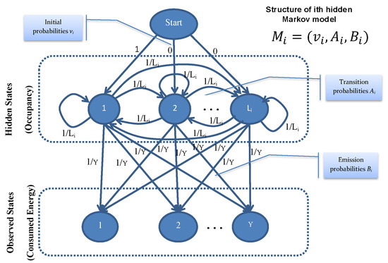
Figure 2. Hidden Markov Model components and internal structure after initialization (before training).

For HHM models generation and training, we have used hourly energy consumption data collected from smart meters installed in the selected residential building of Seoul, South Korea for period of one (01) year. Through data transformation process, we convert the hourly energy consumption data to get floor-wise occupancy sequence. Details about data transformation process is provided in Section 5. Through this transformation, we get numerous different combinations for occupancy sequence. With every occupancy sequence, we have associated a class label based on total energy consumption. It is quite understandable that same occupancy sequence may result in different total energy consumption on different floors, on different days, on different timings.

Let S be our set of all occupancy sequences. For every $s\in S$, we have corresponding class label for energy consumption i.e., $E_s$. Depending upon the unique values in the input sequence, we also assign a state label to each sequence $L_s$. Let, T be the total number of classes in our data where each class corresponds to a unique combination of $E_s$ and $L_s$. Similarly, we can express a total number of unique labels for energy consumption as Y (irrespective of occupancy sequence). A brief description of the terms used in our HMM is given in Table 1.

Table 1. Brief description of terms used in our HMM.

Term	Variable	Value/Size	Description
Data	S	8760	Total size of input data is = 365 days × 24 h per day = 8760
Sequence	s	e.g., 1-2-3 …2	This sequence is obtained after transformation and is used
			as input to our HMM. We have total 8760 input sequences.
Energy Label	$E_s$	e.g., E34	Energy consumption for each sequences.
State Label	$L_s$	e.g., 4	Number of unique values in corresponding input sequence.
Classes	T	e.g., 108	Total number of unique combinations of $E_s$ and $L_s$.
Symbols	Y	e.g., 42	Total number of unique labels in $E_s$.
hmmc	hmmc	e.g., 108	Array of HMM models created.

There are three main phases:

3.1. HMM Models Creation and Initialization

First, we create desired number of HMMs for the available dataset. Total 108 different models are created as we have 108 unique combinations of class and state labels in our dataset. All these models are initialized with starting transition and emission probabilities and finally stored in $hmmc$ structure. Let $M_i$ be the ith HMM model which is expressed as below:

$$M_i=(v_i,A_i,B_i)$$

(1)

where $v_i$ is the state probabilities vector, $A_i$ is the inter-state transition probabilities and $B_i$ is the emission probabilities. These probabilities vectors/matrices are initialized as below:

$$v_i\left[0\right]=1\mathrm{and}{v}_i\left[j\right]=0\forall j\in \left\{1,\dots ,L_i\right\}$$

(2)

where $L_i$ is number of unique values in corresponding input sequence s.

$$A_i[j,k]=\frac{1}{L_i}\forall j,k\in \left\{1,\dots ,L_i\right\}$$

(3)

$$B_i[p,q]=\frac{1}{Y}\forall p\in \left\{1,\dots ,L_i\right\},q\in \left\{1,\dots ,Y\right\}$$

(4)

Above scheme ensure summation of all row vectors to be 1 to satisfy Markov condition. Figure 2 shows the typical structure of ith HMM model after initialization.

3.2. HMM Models Training

In the second phase, we train the models with the available dataset. For every unique combination of energy label $E_s$ and state label $L_s$, we have created a hidden Markov model with initial probabilities as shown in Figure 2. For training of each specific model, first, we extract set of corresponding input sequences that have same energy label $E_s$ and state label $L_s$. Baum-Welch algorithm is used for training of HMMs [34]. For given set of training observation sequences and initial structure of HMM (numbers of hidden and visible states), Baum-Welch algorithm determines HMM parameters (state transition and emission probabilities) that best fit to the training data. After, model training, these probabilities are replaced with system steady-state probabilities for each model. Flowchart given in Figure 3 explains the initialization and training process of our HMMs.

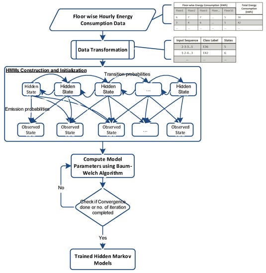
Figure 3. Flowchart of HMMs construction, initialization and training.

3.3. Prediction using HMM Models

Finally, we perform prediction for every input sequence to compute predicted energy consumption. Here, we compute the likelihood (probability) of every trained HMM model for generating the given input sequence using Baum-Welch’s forward algorithm. As we have created T HMMs and each model is trained for a particular energy consumption (energy label) using corresponding estimated occupancy sequence. Thus, for any given occupancy sequence s, we will compute the likelihood for every ith model to generate given input observation sequence i.e., $P_i=M_i\left(s\right)$. The model with maximum likelihood will be selected and its corresponding energy label will be considered as predicted energy consumption as shown in Figure 4.

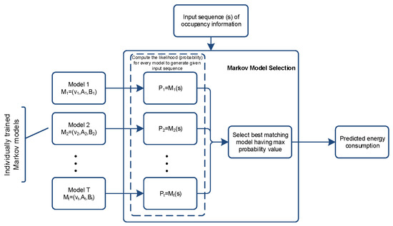
Figure 4. Energy prediction from observed occupancy data using Hidden Markov Model.

Figure 5 presents pseudo-code for HMM creation, training and testing based on Accord.NET framework [33].

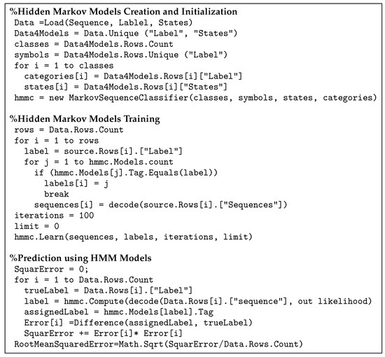
Figure 5. Pseudo-code for HMM creation, training and testing based on Accord.NET framework.

4. Proposed Energy Prediction Model Using HMM

Figure 6 presents the architecture of our proposed system for prediction of energy consumption in smart buildings based on Hidden Markov Model. System functionality is covered in four layers, each having designated components for a specific task. Brief description of each layer is given below.

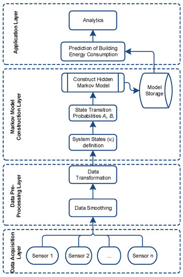
Figure 6. Proposed energy prediction model using HMM.

4.1. Data Acquisition Layer

This layer composed of physical IoT devices including various sensors and actuators. Sensors are used to collect contextual information e.g., environmental conditions, temperature, humidity, user occupancy, etc. To detect user occupancy, various Passive Infra-Red (PIR) sensors can be used to get binary information about occupancy i.e., occupied or not occupied. To get actual user count, cameras will be required to install on transition point between various zones of the building. After processing of the collected data, home appliances can be controlled accordingly by sending control commands to the actuators. For theses experiments, we have only used the energy consumption data collected via smart meters installed on each floor of selected four buildings. Energy consumption data is recorded on hourly interval basis for a period of one year i.e., from 1 January 2010 to 31 December 2010. Figure 7 provides 2 days sample view of collected data for a single building having 33 floors.

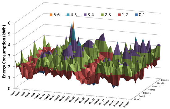
Figure 7. Sample data (two days) of hourly energy consumption in Building-$IV$.

4.2. Pre-processing Layer

In this layer, we perform some data transformation operation in order to get the data in the format required by the upper layer. This also includes data smoothing filters in order to reduce the number of states in our Markov model. Furthermore, smoothing helps in removing the outliers and anomalies from the data. Various smoothing filters can be used for this purpose e.g., moving average, loess, lowess robust loess/lowess etc. Detailed discussion on data transformation is given in next Section 5.

4.3. Markov Model Construction Layer

This is the most important layer where we construct hidden Markov models in order to perform energy prediction. First, we obtained the observed state’s information from given data and then interstate transition probabilities are calculated using hourly data. Detailed discussion on model creation, state transition and emission probabilities calculations along with model training is covered in Section 3. Once, Hidden Markov Models (HMM) are trained then they are stored in memory for onward usage by the upper application layer.

4.4. Application Layer

In this layer, we use the trained HMM for given sequence of observed data to get the best matching HMM. Depending upon the dataset, we obtain T different Markov models; each model is trained rigorously for a particular type of input sequence. For a given input sequence of occupancy information, each individual model matching is calculated. Finally, the best matching model is selected and its output is considered as predicted energy consumption as shown in Figure 4. We also compare our predicted energy consumption result with actual data to compute mean squared error.

5. Data Collection and Transformation

Given the occupancy pattern information, we can predict energy consumption. In the available data, we have floor-wise hourly energy consumption information collected from smart meters installed in the selected residential building of Seoul, South Korea for period of one (01) year i.e., January 2010 to December 2010. To have an idea about dataset, hourly energy consumption distribution for complete data-set is provided in Figure 8 in the form of box plot. We can easily figure out from the box plot that energy consumption is low in early morning and afternoon where peak energy consumption is observed during noon and night timings. This is due to the fact that residential buildings have maximum occupancy during noon and night times which results in higher energy consumption. This also indicates that there is a strong positive correlation between energy consumption and occupancy in the collected dataset.

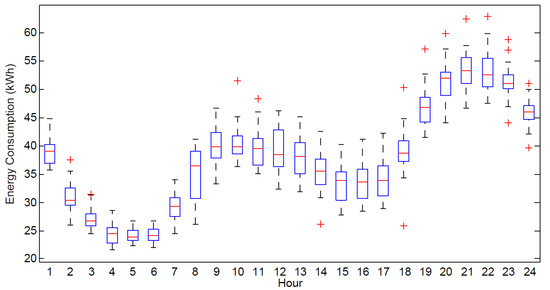
Figure 8. Hourly distribution of energy consumption data for complete data-set.

We can relate user occupancy data with hourly energy consumption by using simple linear transformation but we cannot directly conclude total energy consumption from given occupancy information. For example, two rooms having same user occupancy but different electrical equipment will have different energy consumption ratio. However, if we can have user occupancy pattern then we can predict total energy consumption. Therefore, we need to transform the existing data into a sequence in order to get observation sequence for our Hidden Markov Model. As we observed from data that there is a strong positive correlation between energy consumption and occupancy, so mathematically we can express it as below.

$$Energ{y}_{F_i}=C\times Occu{p}_{F_i}$$

(5)

where $Energ{y}_{F_i}$ is energy consumption at ith floor, $Occu{p}_{F_i}$ is estimated occupancy of the ith floor and C is proportionality constant i.e., per occupant per hour energy consumption. Assuming per person per hour power consumption to be about 10 kWh (approximately), we consider $C=10$ in these experiments. Using a different value of C will results in a different observation sequence for HMM but it will rarely affect the model results as the output (i.e., total energy consumption) remains the same for which model is trained. To get estimated occupancy information from consumed energy, we can re-write Equation (6) as below.

$$Occu{p}_{F_i}=\frac{Energ{y}_{F_i}}{C}$$

(6)

Afterwards, we apply data smoothing filter in order to reduce the number of state transitions using moving average filter with a span of 3 using Equation (7).

$$y_s\left(x\right)=\frac{\left(y(x-1)+y\left(x\right)+y(x+1)\right)}{3}$$

(7)

After smoothing filter operation, the resultant data has a fractional part which is simply removed by rounding the data to the nearest integer value as each value form a state in Markov model. Table 2 illustrate these operations on sample data. Number of states are calculated by computing the unique values in input data sequence and state transitions are calculated by counting the number of state changes while moving from left to right of input data sequence. We can see that after smoothing, the number of states reduced from 5 to 4 and inter-state transitions from 7 to 5 for this sample data.

Table 2. Illustration of smoothing filter operation on a sample occupancy sequence.

Description	Input Data Sequence									Required Number of
										States	Transitions
Sample Data	6	7	7	8	9	6	7	6	5	5	7
Moving Avg. (span = 3)	6.00	6.67	7.33	8.00	7.67	7.33	6.33	6.00	5.00
Rounding to nearest Integer value	6	7	7	8	8	7	6	6	5	4	5

Finally, we get user occupancy data as an observation sequence and for which we use Hidden Markov Model to predict energy consumption as shown in Figure 9. Floor-wise per hour energy consumption data gives us user occupancy pattern in the building which serves as input (observation sequence) to our Markov model whereas total energy consumption for a particular input pattern is associated with the model as a tag which is also referred as a predicted class label.

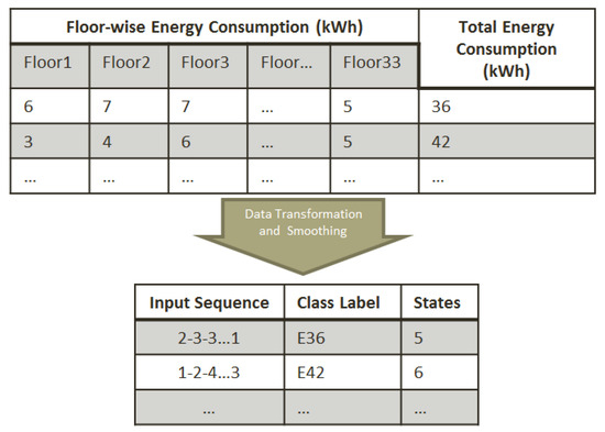
Figure 9. Illustration of data transformation-sample data (per hour energy consumption) to occupancy sequence with corresponding class and state labels.

For each input sequence, we have defined a class label, depending upon the total energy consumption for corresponding input sequence e.g., if total energy consumption for a particular input sequence is N (say N=36) then we assign that sequence with a class label as EN i.e., E36. Furthermore, for every input sequence, we also record a state count i.e., the number of unique values in corresponding input sequence as shown in the third column in Figure 9.

6. Experiments and Results

6.1. Model Validation

For model validation and experimental analysis, we have used real data collected from smart meters installed in the four selected multi-storied residential buildings of Seoul, South Korea for period of one (01) year i.e., 1 January 2010 to 31 December 2010. The number of floors in each building are 33, 15, 36 and 33, respectively. Smart meters are installed at each floor sub-distribution switchboard and are connected to the main Server. Energy consumption data is recorded on hourly interval basis for the stated period of one year and the unit of measurement used for energy consumption is kilowatt-hour (kWh). The dataset has floor-wise hourly energy consumption information for selected four residential buildings. Sample view of collected data for two days is provided in Figure 7 for an anonymous building-$IV$ having 33 floors. This is just to give an idea about data distribution. Furthermore, hourly energy consumption distribution for complete data-set is shown in Figure 8 in the form of box plot.

For these experiments, we have used 70% of available data for training and rest of the 30% is used for testing. Figure 10 shows comparison results of predicted energy consumption with original data values for the testing dataset. The results show that both lines are almost going side by side which indicates that our prediction algorithm is working nicely. To get better insight, we present absolute error difference results in Figure 11. Absolute error in prediction graph reveals that most of the values lie within $[-4,+4]$. Root mean squared error (RMSE) for the given result is 2.62 which is quite reasonable. These results not only validate the model but also gives us the confidence to perform a comparative analysis with other prediction algorithms.

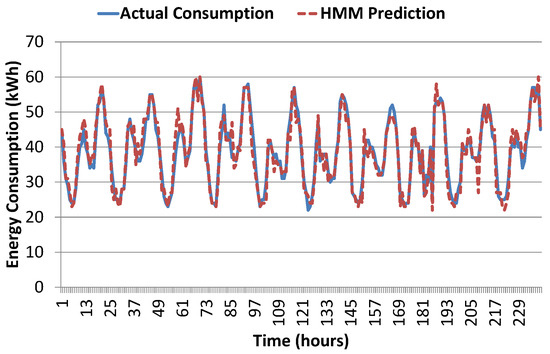
Figure 10. Proposed model prediction results in comparison with actual consumption for 10 days hourly data.

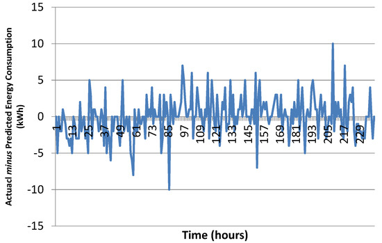
Figure 11. Error in prediction results of the proposed model for 10 days hourly data (RMSE = 2.62).

6.2. Comparative Analysis

For purpose of comparative analysis, we choose three algorithms i.e., Artificial Neural Network (ANN) [35], Support Vector Machine (SVM) [36], and Classification and Regression Trees (CART) [37]. These three algorithms were applied on the same datasets to compute predicted energy consumption. Configuration settings used for ANN, SVM and CART algorithm are given below.

6.2.1. Artificial Neural Network (ANN)

We have used default Feed Forward Neural Network available in MATLAB 2013a [38] with Levenberg-Marquardt training method having 4 input features i.e., hourly data along with weekly, weekday and monthly information. ANN implementations available in Matlab provide automatic scaling of input data into $[-1,+1]$. As we have used the default implementation of ANN available in Matlab, therefore we need not pre-process the input data. Levenberg-Marquardt training algorithm is selected because it is considered to be the best and fastest method for moderate size neural networks. The output of the neural network is predicted consumed energy. We have used tan-sigmoid(x) as our activation function at the hidden layer and linear function at the output layer. Different models of ANN are tested with varying number of neurons in the hidden layer from 4 to 30. Parameters of ANN algorithm are fine-tuned and the reported results are the best that we obtained after a number of repeated experiments. Screenshot of AAN configuration given in Figure 12 taken when training process was completed. Maximum number of epochs used to train the network is 100.

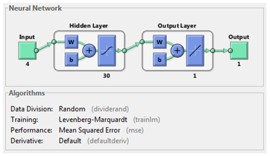
Figure 12. Screenshot of ANN configurations used for prediction of energy consumption.

6.2.2. Support Vector Machine (SVM)

SVM is another very popular algorithm that was initially developed for binary classification problems [39]. Currently, its many variations are available to solve complex classification and regression problems [36,40] using kernel tricks. Depending upon problem input size and nature, appropriate kernel function can be selected among linear, polynomial, radial, etc. For kernel selection, we performed experiments with three different kernels i.e., linear, polynomial and radial basis function (RBF). Results with linear kernel were the best and are reported in this paper. In these experiments, we have used default model of SVM in MATLAB 2017b [41] with sequential minimal optimization (SMO) optimizer and box constraint $C=1$, The model converged after 25,000 iterations with $ϵ=1.49$. Parameters of SVM algorithm are fine-tuned and the reported results are the best that we obtained after a number of repeated experiments. SVM implementations available in Matlab provide automatic scaling of input data into $[-1,+1]$, therefore we need not pre-process the input data for SVM algorithm.

6.2.3. Classification and Regression Trees (CART)

For CART, we also use default CART implementation available in MATLAB 2013a [38]. CART decision is created using regression method. Default regression tree has 120 levels and best prediction results were obtained with pruning last 5 levels. Like ANN and SVM, parameters for CART algorithm are fine-tuned and the reported results are the best that we obtained after a number of repeated experiments. Screenshot of pruned CART tree obtained for prediction of energy consumption is given in Figure 13.

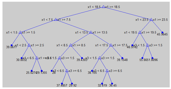
Figure 13. Screenshot of pruned CART tree used for prediction of energy consumption.

Absolute error in prediction results of our proposed model together with ANN, SVM and CART results is shown in Figure 14. It can be seen that results of all the four algorithms look quite similar. Significant difference is not visible from this figure. Just like results of the proposed model, absolute error in prediction for SVM, ANN and CART also remain within $[-4,+4]$ for most of the values and there seems no significant difference. In such cases, when the difference is not obvious from graphs/plots then statistical measures are very useful. These measures not only summarize the data but also help in analyzing the data by quantifying the accuracy of results. Thus, it can reveal the relative difference which may not be visible, otherwise.

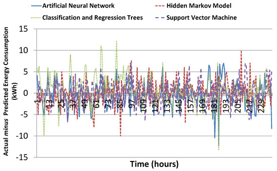
Figure 14. Error in prediction results of the proposed model, ANN, SVM and CART algorithm for 10 days hourly data.

6.3. Statistical Measures used for Comparison

Brief description and formula of four statistical measures used for comparative analysis are given below.

• Mean Absolute Deviation (MAD): This is the sum of absolute differences between the actual and predicted value, divided by the number of data items.

  $$MAD=\frac{{\sum }_{i=1}^n\left|D_i-{\widehat{D}}_i\right|}{n}$$

  (8)
• Mean Squared Error (MSE): This is the most widely used error metric. It penalizes more when error gets increased as squaring a number grows exponentially from small to big numbers. The $MSE$ is calculated by adding the squared errors and dividing it by the number of data items.

  $$MSE=\frac{{\sum }_{i=1}^n{\left(D_i-{\widehat{D}}_i\right)}^2}{n}$$

  (9)
• Root Mean Square Error (RMSE): This is obtained by taking the square root of $MSE$.

  $$RMSE=\sqrt{\frac{{\sum }_{i=1}^n{\left(D_i-{\widehat{D}}_i\right)}^2}{n}}$$

  (10)
• Mean Absolute Percentage Error (MAPE): This is the average of absolute errors divided by the original values, multiplied by 100 to get result in percentage.

  $$MAPE=\frac{{\sum }_{i=1}^n\left|\frac{D_i-{\widehat{D}}_i}{D_i}\right|}{n}\times 100$$

  (11)

where n is the total number of entries in the testing dataset, $D_i$ is the actual energy consumption (kWh) for ith instance in the dataset and ${\widehat{D}}_i$ is the corresponding predicted energy consumption (kWh). These statistical measures give us a single number to quantify prediction accuracy. If prediction results are more closed to actual energy consumption then corresponding values for these statistical measures will also be small. An algorithm having smallest values for these statistical measures will be the best.

Table 3 presents the statistical summary of the results for comparison among the four algorithms. Proposed model results outperform the other three algorithms on all statistical measures. Artificial neural networks results are second best and it has a very low difference when compared to our hidden Markov model results. Relative accuracy of proposed model results is 2.96% when compared to ANN results in terms of $RMSE$ metric. However, it is $6.09\%$ better than SVM and 9.03% better than CART results. Higher prediction accuracy gives us confidence to further explore application of the proposed model in building control applications for achieving better energy efficiency.

Table 3. Statistical summary of energy consumption prediction (kWh) results using ANN, SVM, CART and Proposed Model.

Statistical Measures	ANN	SVM	CART	Proposed Model
MAD	2.07	2.23	2.19	1.88
MSE	7.32	7.82	8.34	6.91
RMSE	2.70	2.79	2.88	2.62
MAPE	5.66	5.78	5.96	5.22

6.4. Temporal Granularity Analysis

To further establish and validate prediction results of our proposed model, we have performed temporal granularity analysis. Figure 10 shows energy prediction results based on hourly data. Here, we analyze the impact of temporal granularity on the prediction accuracy of our proposed HMM model. For this purpose, we have performed daily and weekly data aggregation. Figure 15 and Figure 16 show the prediction results for daily and weekly aggregated data. Prediction accuracy in terms of root mean square error metric for hourly, daily and weekly data is 2.62, 1.54 and 0.46 respectively. This shows that our model prediction accuracy improves for coarse grain data. We have also evaluated the performance of other algorithms (ANN, SVM, and CART) for daily and weekly predictions and their results were lower than proposed HMM scheme, therefore not reported in the paper.

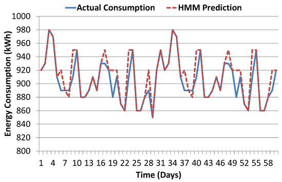
Figure 15. Proposed model prediction results in comparison with actual consumption for two months daily data.

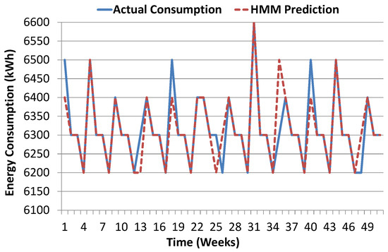
Figure 16. Proposed model prediction results in comparison with actual consumption for one year weekly data.

6.5. Discussion on Results

Overall, our results indicate that our proposed HMM model performs well as compared to ANN, SVM and CART algorithm. For given application scenario, its quite understandable that same observation sequence can result in different energy consumption in different buildings. This is due to the fact that total energy consumption depends not only upon the observation but also the nature of equipment and appliances installed in respective buildings. Like for instance, per hour energy consumption for room A and room B will be different even though both having same number of occupants if different types of appliances are installed in each room. In given application scenario, we can only have information about users occupancy sequence but no information about the details of appliance installed on each floor. Furthermore, HMM works well to discover the underlying structure and information and thus results in better prediction accuracy as compared to ANN, SVM and CART because HMM model uses the extra state information along with observation sequence and total energy consumption. A separate HMM model is trained for every unique combination of total energy consumption and states information which helps HMM model to accurately predict energy consumption for a given observation sequence.

Furthermore, we observe that our model prediction results for coarse grain data i.e., weekly is much better than the results for fine grain data i.e., hourly. In other words, it is inherently harder to predict at smaller time intervals due to the stochastic nature of energy consumption as for fine grain data, the variation in observation sequence is minor which is difficult to capture. Analyzing the results of HMM model over the larger time interval (daily and weekly) reveals improvement in prediction accuracy in terms of root mean square error metric. This is due to the fact that, for larger time intervals, the variation among individual observation sequences becomes distinct and more visible which is easily captured by HMM. Another reason for the improvement in prediction accuracy for coarse grain data is that the number of observation sample gets reduced. Thus for a relatively smaller number of distinct observation sequences, HMM model is able to produce better results. However, there are some mis-predictions for weekly aggregated data as shown in Figure 16. For sake of illustration, we consider three sample cases for investigation i.e., week-1, week-5, and week-9. These three cases are carefully selected to better analyze the model prediction accuracy. The week-1 case is an example case for mis-prediction. Week-5 and week-9 are example cases for accurate prediction of energy consumption i.e., 6500 kWh and 6400 kWh respectively. Predictions results for week-5 and week-9 are accurate, however, there is some error in prediction for week-1, where predicted energy consumption is 6400 kWh, while actual energy consumption is 6500 kWh as shown in Table 4.

Table 4. Details of three sample cases in weekly data.

Week No.	Observation Seq.	States	Actual Consumption (kWh)	HMM Prediction (kWh)
Week-1	20-14-15-17-14-13 ...22	14	6500	6400
Week-5	19-14-15-17-15-13 ...21	15	6500	6500
Week-9	21-13-15-17-14-12 ...22	15	6400	6400

It is evident from Table 4 that all three weeks’ data is different. Here, the week-1 case is unique due to a different number of states as compared to week-5 and week-9. Our proposed algorithm has predicted total energy consumption of 6400 kWh for week-1 which means that week-1’s observation sequence is more like week-9’s observation sequence. To further validate this assertion, we have cross-checked similarity indexes of the three cases and its results are shown in Table 5.

Table 5. Pairwise cosine-similarity among selected three weeks observation sequence.

	Week-1	Week-5	Week-9
Week-1	1	0.9987	0.9991
Week-5	0.9987	1	0.999
Week-9	0.9991	0.999	1

Overall, similarity index values in Table 5 indicate that all three cases are highly similar and there is a minor difference between them. However, contrasting cosine-similarity between week-1↔week-5 and week-1↔week-9, we can see that the week-1 case has relatively more resemblance to week-9 as compared to week-5, therefore total energy prediction results for week-1 case are same as week-9. This also signifies that our proposed model is able to capture the minute difference of $0.0004$ and accurately relate week-1 to week-9 which results in mis-prediction, unfortunately.

7. Conclusions and Future Work

In this paper, we have presented a hidden Markov model-based algorithm for prediction of energy consumption in smart buildings. We have used real data collected through smart meters in selected buildings at Seoul, South Korea for model validation and results analysis. Proposed model prediction results are compared with three well-known prediction algorithms i.e., ANN, SVM, and CART. Statistical analysis shows that our proposed model results are 2.96% better than ANN results in terms of RMSE metric, $6.09\%$ better than SVM and 9.03% better than CART results. To further establish and validate prediction results of our proposed model, we have performed temporal granularity analysis. For this purpose, we have evaluated its results for hourly, daily and weekly data aggregation. Prediction accuracy in terms of root mean square error metric for hourly, daily and weekly data is 2.62, 1.54 and 0.46 respectively. This shows that our model prediction accuracy improves for coarse grain data. Higher prediction accuracy gives us the confidence to explore proposed model application in building control systems for achieving better energy efficiency. We have selected HMM for prediction due to its inherent benefits over other AI-based algorithms. HMM-based trained models can be used to identify underlying appliances used from cumulative energy consumed. Furthermore, HMM models can perform automated fault monitoring and appliances health assessment by performing analysis of individual device energy consumption pattern. At the first step, we tried to establish that HMM models can accurately predict energy consumption which was the subject matter of this paper. These initial results give us confidence and we are currently exploring various alternatives and collecting data to extend this work in aforementioned directions.

References

- Selin, R. The Outlook for Energy: A View to 2040; ExxonMobil: Irving, TX, USA, 2013. [Google Scholar]
- Sieminski, A. International energy outlook. In Energy Information Administration (EIA); Energy Information Administration: Washington, DC, USA, 2014. [Google Scholar]
- Sethi, P.; Sarangi, S.R. Internet of Things: Architectures, Protocols, and Applications. J. Electr. Comput. Eng. 2017, 2017. [Google Scholar] [CrossRef]
- Kim, S.; Kim, S. A multi-criteria approach toward discovering killer IoT application in Korea. Technol. Forecast. Soc. Chang. 2016, 102, 143–155. [Google Scholar] [CrossRef]
- Li, X.; Lu, R.; Liang, X.; Shen, X.; Chen, J.; Lin, X. Smart community: an internet of things application. IEEE Commun. Mag. 2011, 49, 68–75. [Google Scholar] [CrossRef]
- Trends in Global Energy Efficiency, Energy Efficiency Report, South Korea. Source Enerdata, 2011. Available online: https://www.enerdata.net/publications/reports-presentations/ (accessed on 20 August 2017).
- Ali, S.; Kim, D.H. Optimized Power Control Methodology Using Genetic Algorithm. Wirel. Pers. Commun. 2015, 83, 493–505. [Google Scholar] [CrossRef]
- Ali, S.; Kim, D.H. Effective and Comfortable Power Control Model Using Kalman Filter for Building Energy Management. Wirel. Pers. Commun. 2013, 73, 1439–1453. [Google Scholar] [CrossRef]
- Wang, Z.; Yang, R.; Wang, L. Multi-agent control system with intelligent optimization for smart and energy-efficient buildings. In Proceedings of the IECON 2010-36th Annual Conference on IEEE Industrial Electronics Society, Glendale, AZ, USA, 7–10 November 2010; pp. 1144–1149. [Google Scholar]
- Levermore, G.J. Building Energy Management Systems: Applications to Low Energy HVAC and Natural Ventilation Control; E & FN Spon: London, UK; New York, NY, USA, 2000. [Google Scholar]
- Benard, C.; Guerrier, B.; Rosset-Louerat, M.M. Optimal Building Energy Management: Part II—Control. J. Sol. Energy Eng. 1992, 114, 13–22. [Google Scholar] [CrossRef]
- Curtiss, P.S.; Shavit, G.; Kreider, J.F. Neural networks applied to buildings—A tutorial and case studies in prediction and adaptive control. ASHRAE Trans. 1996, 102, 1141–1146. [Google Scholar]
- Ahmad, A.; Hassan, M.; Abdullah, M.; Rahman, H.; Hussin, F.; Abdullah, H.; Saidur, R. A review on applications of ANN and SVM for building electrical energy consumption forecasting. Renew. Sustain. Energy Rev. 2014, 33, 102–109. [Google Scholar] [CrossRef]
- Kusiak, A.; Li, M.; Zhang, Z. A data-driven approach for steam load prediction in buildings. Appl. Energy 2010, 87, 925–933. [Google Scholar] [CrossRef]
- Siroky, J.; Oldewurtel, F.; Cigler, J.; Privara, S. Experimental analysis of model predictive control for an energy efficient building heating system. Appl. Energy 2011, 88, 3079–3087. [Google Scholar] [CrossRef]
- Wang, Z.; Wang, L.; Dounis, A.I.; Yang, R. Multi-agent control system with information fusion based comfort model for smart buildings. Appl. Energy 2012, 99, 247–254. [Google Scholar] [CrossRef]
- Edwards, R.E.; New, J.; Parker, L.E. Predicting future hourly residential electrical consumption: A machine learning case study. Energy Build. 2012, 49, 591–603. [Google Scholar] [CrossRef]
- Crawley, D.B.; Hand, J.W.; Kummert, M.; Griffith, B.T. Contrasting the capabilities of building energy performance simulation programs. Build. Environ. 2008, 43, 661–673. [Google Scholar] [CrossRef]
- Amasyali, K.; El-Gohary, N.M. A review of data-driven building energy consumption prediction studies. Renew. Sustain. Energy Rev. 2018, 81, 1192–1205. [Google Scholar] [CrossRef]
- Karatasou, S.; Santamouris, M.; Geros, V. Modeling and predicting building’s energy use with artificial neural networks: Methods and results. Energy Build. 2006, 38, 949–958. [Google Scholar] [CrossRef]
- Li, K.; Su, H.; Chu, J. Forecasting building energy consumption using neural networks and hybrid neuro-fuzzy system: A comparative study. Energy Build. 2011, 43, 2893–2899. [Google Scholar] [CrossRef]
- Ali, S.; Kim, D. Enhanced power control model based on hybrid prediction and preprocessing/post-processing. J. Intell. Fuzzy Syst. 2016, 30, 3399–3410. [Google Scholar] [CrossRef]
- Kalogirou, S.; Neocleous, C.; Schizas, C. Building heating load estimation using artificial neural networks. In Proceedings of the Clima 2000 Conference, Brussels, Belgium, 30 August–2 September 1997; Volume 8, p. 14. [Google Scholar]
- Olofsson, T.; Andersson, S. Long-term energy demand predictions based on short-term measured data. Energy Build. 2001, 33, 85–91. [Google Scholar] [CrossRef]
- Goodwin, M.; Yazidi, A. A pattern recognition approach for peak prediction of electrical consumption. Integr. Comput. Aided Eng. 2016, 23, 101–113. [Google Scholar] [CrossRef]
- Kalogirou, S.A. Artificial neural networks in energy applications in buildings. Int. J. Low Carbon Technol. 2006, 1, 201–216. [Google Scholar] [CrossRef]
- Erickson, V.L.; Carreira-Perpinan, M.A.; Cerpa, A.E. OBSERVE: Occupancy-based system for efficient reduction of HVAC energy. In Proceedings of the 10th ACM/IEEE International Conference on Information Processing in Sensor Networks, Chicago, IL, USA, 12–14 April 2011; pp. 258–269. [Google Scholar]
- Adamopoulou, A.A.; Tryferidis, A.M.; Tzovaras, D.K. A context-aware method for building occupancy prediction. Energy Build. 2016, 110, 229–244. [Google Scholar] [CrossRef]
- Zia, T.; Bruckner, D.; Zaidi, A. A hidden markov model based procedure for identifying household electric loads. In Proceedings of the IECON 2011-37th Annual Conference on IEEE Industrial Electronics Society, Melbourne, Australia, 7–10 November 2011; pp. 3218–3223. [Google Scholar]
- Hu, P.; Zhou, Z.; Liu, Q.; Li, F. The HMM-based modeling for the energy level prediction in wireless sensor networks. In Proceedings of the 2nd IEEE Conference on Industrial Electronics and Applications, Harbin, China, 23–25 May 2007; pp. 2253–2258. [Google Scholar]
- Mueller, J.A.; Kimball, J.W. An Accurate Method of Energy Use Prediction for Systems with Known Composition. In Proceedings of the 3rd International Workshop on NILM, Vancouver, BC, Canada, 14–15 May 2016. [Google Scholar]
- González, A.M.; Roque, A.S.; García-González, J. Modeling and forecasting electricity prices with input/output hidden Markov models. IEEE Trans. Power Syst. 2005, 20, 13–24. [Google Scholar]
- Accord.NET Framework for C#. Available online: http://accord-framework.net/index.html/ (accessed on 16 December 2016).
- Sammut, C.; Webb, G.I. (Eds.) Baum-Welch Algorithm. In Encyclopedia of Machine Learning; Springer: Boston, MA, USA, 2010; p. 74. [Google Scholar]
- Bebis, G.; Georgiopoulos, M. Feed-forward neural networks. IEEE Potentials 1994, 13, 27–31. [Google Scholar] [CrossRef]
- Krammer, K.; Singer, Y. On the algorithmic implementation of multi-class SVMs. Proc. JMLR 2001, 2, 265–292. [Google Scholar]
- Breiman, L.; Friedman, J.; Stone, C.J.; Olshen, R.A. Classification and Regression Trees; CRC Press: Boca Raton, FL, USA, 1984. [Google Scholar]
- MATLAB. version 8.1.0 (R2013a); The MathWorks Inc.: Natick, MA, USA, 2013. [Google Scholar]
- Boser, B.E.; Guyon, I.M.; Vapnik, V.N. A training algorithm for optimal margin classifiers. In Proceedings of the Fifth Annual Workshop on Computational Learning Theory, Pittsburgh, PA, USA, 27–29 July 1992; pp. 144–152. [Google Scholar]
- Gunn, S.R. Support vector machines for classification and regression. ISIS Tech. Rep. 1998, 14, 5–16. [Google Scholar]
- MATLAB. version 9.3.0 (R2017b); The MathWorks Inc.: Natick, MA, USA, 2017. [Google Scholar]
© 2018 by the authors. Licensee MDPI, Basel, Switzerland. This article is an open access article distributed under the terms and conditions of the Creative Commons Attribution (CC BY) license (http://creativecommons.org/licenses/by/4.0/).