Ultra-Short-Term Wind Power Prediction Based on Multivariate Phase Space Reconstruction and Multivariate Linear Regression

Abstract

In order to improve the accuracy of wind power prediction (WPP), we propose a WPP based on multivariate phase space reconstruction (MPSR) and multivariate linear regression (MLR). Firstly, the multivariate time series (TS) are constructed through reasonable selection of wind power and weather factors, which are closely associated with wind power. Secondly, the phase space of the multivariate time series is reconstructed based on the chaos theory and C-C method. Thirdly, an auto regression model for multivariate phase space is created by regarding phase variables as state variables, and the very-short-term wind power is predicted by using a multi-linear regression algorithm. Finally, a parallel algorithm based on map/reduce is presented to improve computing speed. A cloud computing platform, Hadoop consisting of five nodes, is established as a matter of convenience, followed by the prediction of wind power of a wind farm in the Hunan province of China. The experimental results show that the model based on MPSR and MLR is more accurate than both the continuous method and the simple approximation method, and the parallel algorithm based on map/reduce effectively accelerates the computing speed.

1. Introduction

In the past decades, with the increasing population, industrial need, and energy need [1], a large amount of fuels such as fossil oil, coal, and natural gas have been consumed. However, the fossil fuels can discharge a large amount of greenhouse gas and pollute the environment. What is more, the fossil fuels are non-renewable and diminishing day-by-day. Therefore, researchers have focused on the renewable energy sources, among which wind power generation is one of the most mature renewable energies with lower pollution and greenhouse gas emissions [2]. Wind power generation is affected by wind speed, wind direction, temperature, turbine type, terrain roughness, air density, and so on [3]. The wind power is random and intermittent. To reduce the risk that is caused by the wind power’s fluctuation, both a one-day-ahead (0–24 h) and a real-time (15 min–4 h) wind power predicting report should be submitted to the Grid Dispatch Center in China. Actually, the ultra-short-term wind power prediction (UST-WPP) has been extensively employed in many fields, such as balancing load, optimal operation of reserves [4], and wind farm control [5]. The wind farm owners, power users, and facilities benefit from an improved wind power prediction (WPP).

According to the current law in China, the wind power prediction with horizons of 1–4 h and 24 h are necessary. This paper focuses on forecasting wind power with short horizons. Specifically, we propose a distributed model for ultra-short-term WPP based on multivariate phase space reconstruction (MPSR) and multivariate linear regression (MLR). Compared with other approaches for short-term wind power prediction, such as artificial neural networks (ANNs), support vector machine (SVM) and single-variable phase space reconstruction, the proposed wind power prediction model is more precise and quicker.

The remainder of this paper is organized as follows. The background of our work is introduced in Section 1. Section 2 reviews the related work. The prepared knowledge is given and the parallel model is proposed in Section 3. Section 4 expresses the key points of the parallel algorithm based on map/reduce. Section 5 describes the prediction experiments. Section 6 outlines the conclusions.

2. Related Works

According to the time horizons, WPP is divided into four categories: long-term prediction, medium-term prediction, short-term prediction, and ultra-short-term prediction [6]. The time horizon and application of the special wind power prediction is shown as Table 1.

Table 1. Classification of wind power prediction based on time horizon.

No.	Method	Time Horizon	Application
1	Long-term	Year	- planning wind farms - Planning of annual generation
2	Medium-term	Week or Month	- Scheduling maintenance
3	Short-term	3 days	- Reducing the discarded wind power - Optimizing the maintenance scheduling - Optimizing the generation scheduling
4	Ultra-short-term	4 h	- Optimizing the frequency - Optimizing the spinning reserve capacity - Optimizing the unit commitment online

The long-term and medium-term wind power predictions do not require very high forecasting accuracy. The short-term WPP forecasts the wind power in next three days and needs more precise results [7], while the ultra-short-term WPP, whose temporal resolution is 15 min, predicts the wind power in next 4 h and requires the highest precision [1]. It is very difficult to accurately forecast wind power because of its chaotic and stochastic characteristics. Additionally, compared to other WPP, the ultra-short-term WPP is more difficult due to its shorter time frames [7]. In the past decades, extensive efforts have focused on WPP, and a large number of wind power prediction methods, models, and tools have been developed. Generally, the WPP methods includes five categories: (a) physical methods, (b) statistic methods, (c) artificial intelligent methods, (d) hybrid methods, and (e) spatio-temporal methods [8].

The physical methods forecast the wind power in terms of the meteorological parameters such as topography, temperature, pressure, wind speed, and wind direction. The well-known physical wind power prediction systems are Prediktor system [9], Previento, and eWind. However, the physical methods are suitable to predict the wind power in 6–72 h or long-term wind power due to the low update frequency of numerical weather prediction (NWP). Because of the high computational cost of NWP, the physical models’ application to ultra-short-term WPP are limited. The hybrid methods, which improve the WPP by making use of the advantages of physical methods, statistical methods, and intelligent methods, are gaining attention. Mehmet Baris Ozkan and Pinar Karagoz presented a novel wind power forecast model: Statistical Hybrid Wind Power Forecast Technique (SHWPFT). Compared with other statistical and physical models such as ANNs and SVM, SHWPFT requires less historical data to establish a model [10]. A hybrid forecasting model based on grey relational analysis and wind speed distributional features is presented to improve the effects of the ultra-short-term WPP [11]. Reference [12] provides an approach of short-term WPP with multiple observation points. The speed and direction of wind are used to forecast the wind power; unfortunately, the error of numeric weather prediction (NWP) must be considered. Since the hybrid models also require the NWP, their application to ultra-short-term WPP is limited too. The statistical methods are widely used for the shorter-term wind power prediction because of the lower computational complexity and cost.

The statistical models can be modified based on the allocation and features of wind farms, and statistical models are widely used to forecast short-term wind power. Generally, the statistical models include the direct prediction and the indirect prediction. The wind speed is forecasted first and then is mapped to the wind power according to the wind power curve in indirect wind power prediction. However, the wind power curve is influenced by the environmental and meteorological variables, which are not considered in indirect methods. Consequently, the accuracy of indirect methods is limited. In direct methods, the wind power is predicted directly according to the historical data, and the wind power predictions have greater accuracy [13]. The statistical models are divided into time series (TS) methods and artificial intelligence (AI) methods. Persistence method is a classical TS method, and it assumes that the wind power at time ‘$t+\Delta t$’ equals the wind power at time ‘t’. Persistence method is more accurate than most physical and other statistical methods in short-term or ultra-short-term WPP. Hence, any new predicting method should be tested against the classical benchmark (persistence method). The other well-known TS models includes autoregressive (AR), autoregressive moving average (ARMA), autoregressive integrated moving average (ARIMA), and so on. However, these TS models are linear and it is difficult to capture the non-linear patterns. It is too difficult to directly create precise mathematical models for wind power prediction because of wind’s complexity, so the artificial intelligence and machine learning methods are employed to improve WPP. Artificial neural network (ANN), Bayesian network (BN) and least square support vector regression (LSSVR) are widely used to improve the ultra-short-term WPP. Duehee Lee and Ross Baldick presented an ensemble model for short-term WPP based on Gaussian processes and neural networks [14] from which the predicted wind power and distribution can be obtained. The ensemble model is relatively accurate in the whole forecasting time horizon, and the predicted distribution objectively reflects the real distribution of wind power. The comparative study shows that the neural networks (NNs) outperform the ARIMA in [15]. A short-term WPP model based on wavelet support vector machine is proposed in reference [16], in which a wavelet support vector machine-based (WSVM) approach effectively reduces the negative effects on predicting results induced by errors of NWP data. Additionally, wind power can be forecasted when fewer training samples are accessed. Nevertheless, the universality should be further verified. The least square support vector machine (LSSVM) outperformed the SVM and NNs in terms of the computational complexity and the global convergence [17] in WPP. It is difficult to directly model the wind power time series that is composed of several components with different characteristics. To improve WPP, the wind power time series are decomposed by the wavelet transform (WT), empirical mode decomposition (EMD), and ensemble empirical mode decomposition (EEMD) in the preprocessing stage [18]. Some prior knowledge and assumptions are necessary to determine the mother wavelet in WT. EMD is a data-driven decomposition method, and outperforms WT. Compared with WT, EMD and its variant EEMD have the greatest accuracy. Although the non-linearity of wind power time series can be dealt with using decomposition methods, the chaotic nature of wind power time series can lead to prediction errors [19]. A method of wind power prediction based on chaotic theory and phase space reconstruction is proposed in reference [20]. Reference [13] proposed a short-term WPP framework based on chaotic time series analysis and singular spectrum analysis, and the accuracy is improved by distinguishing the chaotic and non-chaotic components in both decomposition and prediction stages. However, only the historical wind power data are used to forecast wind power in the phase-space-reconstruction-based WPP model.

According to the output, the statistical WPP is divided into probabilistic prediction and point prediction. To deal with wind ramp dynamics, a support-vector-machine-enhanced Markova model (SVMEM) for short-term WPP was presented by Lei Yang, Miao He, and Junshan Zhang et al. in which both distributional predictions and point predictions are derived [21]. Reference [14] has proved that the uncertainty of wind speed satisfies Gaussian distribution with zero mean and heteroscedasticity. An optimal loss function for heteroscedastic regression and a new framework of v-support vector regression (v-SVR) for learning tasks of Gaussian noise with heteroscedasticity were thus developed to improve the situation. Both the wind speed and wind power, however, satisfy other distribution but not the proposed model in reference [22]. The uncertainty of the wind power is modeled by the probabilistic prediction and prediction interval, which are the extension of point prediction. The point prediction is regarded as the most likely wind power. The probabilistic prediction has been applied to power system security [23], various unit commitment strategies [24], and energy storage sizing [25], etc.

The wind power data at each site are self-correlated individually, but also the wind power data at different sites are spatially cross-correlated. A sparsity-controlled vector autoregressive model is introduced to obtain the spatio-temporal wind power prediction in reference [26]. Although, the predicting methods are discussed in batch learning mode, a general overview of wind power prediction is presented in Table 2.

Table 2. The wind power prediction methods. WPP: wind power prediction.

No.	WPP Methods	Remarks
1	Persistence Method	- benchmark method - Very accurate for ultra-short and short term prediction - Low accuracy for drastically fluctuating wind power series
2	Physical Method	- Uses the meteorological and environmental data - Applied to WPP whose time horizon is more than 6 h
3	Time-Series Models	- Accurate for short-term predictions - Cannot model the non-linearity
4	Artificial Intelligence	- Accurate for short-term predictions - Models the non-linearity - Cannot process the chaotic nature
5	Hybrid Method	- Accurate for medium and long term predictions
6	Spatial-Temporal Method	- Accurate for ultra-short-term predictions - Batch learning mode - Cannot update using the latest and real-time information

The high penetration of wind power will definitely affect the reliability and security of the grid due to the fluctuation and randomness of wind power. Compared with the short-term WPP, the ultra-short-term WPP is more effective to solve these problems. Although the above mentioned works contribute a lot to the development of WPP, the ultra-short-term WPP is still a young area and needs more contributions from different areas.

3. Prepare Knowledge and System Modeling

3.1. Time-Series Similarity

Time-series similarity [27,28] is measured with many methods, such as Minkowski distance, Euclidean distance, Pearson coefficient, and dynamic time warping (DTW) distance [29,30]. Compared to other methods, DTW is not sensitive to synchronization and can measure the similarity of time-series with different lengths. Thus, DTW is employed to measure the similarity of numerical weather prediction series. DTW is defined as follows:

Definition 1.

Dynamic time warping (DTW) distance.$X=\{x_1,x_2,\dots ,x_l\}$and$Y=\{y_1,y_2,\dots ,y_n\}$are 2 time-series, where $l$and n are the lengths of time series X and Y, respectively. The DTW between X and Y is defined recursively as Equation (1).

$$D_{dtw}(X,Y)=\{\begin{array}{l}0, if X=Y=\left\{\right\}\\ +\infty , if X=\left\{\right\} and Y\ne \left\{\right\}\\ +\infty , if X\ne \left\{\right\} and Y=\left\{\right\}\\ d(x_1,y_1)+\min \{\begin{array}{l}{D}_{dtw}(rest(X),Y)\\ D_{dtw}(rest(X),rest(Y))\\ D_{dtw}(X,rest(Y))\end{array}\end{array}$$

(1)

where {} indicates empty time-series,$d(x,y)=\left|\right|x,y|{|}_2$is the 2-norm [31] of x and y, and $rest(X)=\{x_2,\dots ,x_l\}$.

Definition 2.

Time-series similarity. X and Y are 2 time-series, and the time-series similarity between X and Y is defined as Equation (2).

$$S(X,Y)=\{\begin{array}{ll}0,& if \theta <D_{dtw}(X,Y)\\ \theta -D_{dtw}(X,Y),& else\end{array}$$

(2)

where$\theta$is a threshold,$D_{dtw}(X,Y)$is the DTW between X and Y.

3.2. Multi-Variable Phase Space Reconstruction

According to Takens-theorem [32,33], the phase space of chaotic time series $x_1,x_2,\dots ,x_n$ is reconstructed with appropriate embedding dimension $m$ and time delay $\tau$; the original system and the trajectory of reconstructed phase space are differential homeomorphism. The phase space reconstruction theory [34] of single-variable chaotic time series could be extended to multi-variable chaotic time series. The multi-variable phase space reconstruction is defined as follows.

Definition 3.

Multi-variable phase space reconstruction. X¹, X², …, X^K are K chaotic time-series, where Xⁱ =$\{x_1^i,x_2^i,\dots ,x_n^i\}$, and i = 1, 2, …, K. The q-th phase point of reconstructed phase space for multi-variable chaotic time series X¹, X², …, X is shown as Equation (3).

$$\begin{array}{l}{V}_q=\{x_q^1,x_{q-{\tau }_1}^1,\dots ,x_{q-(m_1-1){\tau }_1}^1,\\ x_q^2,x_{q-{\tau }_2}^2,\dots ,x_{q-(m_2-1){\tau }_2}^2,\dots ,\\ x_q^K,x_{q-{\tau }_K}^K,\dots ,x_{q-(m_K-1){\tau }_K}^K\}\end{array}$$

(3)

where$q=j,j+1,\dots n,j=\underset{1\le i\le K}{\max }\{(m_i-1){\tau }_i\}+1$and$m_i$and${\tau }_i$are embedding dimension and time delay of the chaotic time-series$X^i$, respectively. The embedding dimension$m_i$and time delay${\tau }_i$are obtained using C-C algorithm [33].

3.3. Ultra-Short-Term WPP Modeling

In this paper the ultra-short-term WPP model is based on multi-variable phase space reconstruction, similarity of time-series, and linear regression. Our forecasting model includes steps steps, which are specifically presented in Figure 1.

Figure 1. Flow diagram of ultra-short-term wind power prediction (WPP).

More details about the proposed ultra-short-term WPP model are listed below.

Step 1: Data preprocessing. The historical wind power data and weather data may be missing for some reason, for instance, equipment failure, network interruption, etc. The continuous missing data series $Md$, whose length is more than 5, is removed from historical data series. Otherwise, data is specified by simple interpolation, as expressed in Equation (4).

$$x_i=x_0+\frac{i\times (x_e-x_s)}{N+1}$$

(4)

where $x_s$ is the data point before $Md$, $x_e$ is the data point behind $Md$, $i=1,2,\dots ,N$, and N is the length of missing data series $Md$.

Step 2: Data dimensionality reduction. NWP includes some important parameters, for instance, wind speed v, wind direction $\theta$, atmospheric pressure p, and temperature t. The speed and direction of wind are shown in Figure 2.

Figure 2. The decomposition of wind speed.

In Figure 2, the x-axis is the latitude line of the given location, and the east is the positive direction. The y-axis is the longitude of the given location, and the north is the positon direction. In order to conveniently forecast wind power, wind speed $\nu$ is decomposed to ${\nu }_x$ and ${\nu }_y$.

$$\begin{array}{l}{\nu }_x=\nu \times \cos \theta \\ {\nu }_y=\nu \times \sin \theta \end{array}$$

(5)

where $\theta$ is the angle between wind direction $\nu$ and the x-axis.

Only the most important parameters (${\nu }_x$, ${\nu }_y$ and p) of NWP are selected in the presented model. The historical NWP data can be expressed as a $N\times 3$ matrix M, which is clearly shown as Equation (6).

$$M=\left(\begin{array}{l}{u}_1,{\nu }_1,p_1\\ u_2,{\nu }_2,p_2\\ \dots \\ u_N,{\nu }_N,p_N\end{array}\right)$$

(6)

where N is the number of NWP data points. The matrix M is converted to a $N\times 1$ matrix using the approach in reference [2], as displayed in Equation (8).

$$C=M^T\times M$$

(7)

$$X=M\times e={\left(w_1, w_2,\dots ,w_N\right)}^T$$

(8)

where e is an eigenvector, whose corresponding Eigen value is the maximal Eigen value of matrix C.

Step 3: The most similar NWP series segments searching: NWP₀ is the NWP data series during 2L hours, which consist of two equal parts, namely, the former L hours and the latter L hours. NWP0 includes 8L data points (4 points per hour). NWP₀ is converted to $X^0$, and the whole historical NWP data series is converted to $X$ according to Equations (6)–(8). $X^{is}$ is the top K sub-series of X, which are most similar to $X^0$, and $S_i$ is the similarity between $X^0$ and $X^{is}$, $i=1,2,\dots ,K$.

Step 4: The phase space reconstruction for multivariate time series. ${\tau }_X$ and ${\tau }_P$ are the delay time of X and P, respectively, and $m_X$ and $m_P$ are the embedding dimensions of X and P, respectively. ${\tau }_X$, ${\tau }_P$, $m_X$ and $m_P$ are achieved by C-C method. $P^i$ and $X^i$ ($i=0,1,\dots ,K$) are the wind power sub-series and reduced NWP sub-series at the same time period, and $P{h}^i$ is the reconstructed phase space of $P^i$ and $X^i$.

Step 5: Multivariate linear regression. The multivariate linear regressions are shown as Equation (9)

$$\left(\begin{array}{l}{y}_1\\ y_2\\ \dots \\ y_m\end{array}\right)=\left(\begin{array}{l}{c}_{1,1},c_{1,2},\dots ,c_{1,m}\\ c_{2,1},c_{2,2},\dots ,c_{2,m}\\ \dots \\ c_{m,1},c_{m,2},\dots ,c_{m,m}\end{array}\right)\ast \left(\begin{array}{l}{x}_1\\ x_2\\ \dots \\ x_m\end{array}\right)+\left(\begin{array}{l}{c}_{1,0}\\ c_{2,0}\\ \dots \\ c_{m,0}\end{array}\right)+\left(\begin{array}{l}{\xi }_1\\ {\xi }_2\\ \dots \\ {\xi }_m\end{array}\right)$$

(9)

where $\xi$ = ${({\xi }_1,{\xi }_2,\dots ,{\xi }_m)}^T$ is residual error, ${(x_1,x_2,\dots ,x_m)}^T$ is the input, and ${(y_1,y_2,\dots ,y_m)}^T$ is the output. The coefficient matrix $C$ and constant term $C_0$ are shown as Equation (10).

$$C=\left(\begin{array}{l}{c}_{1,1},c_{1,2},\dots ,c_{1,m}\\ c_{2,1},c_{2,2},\dots ,c_{2,m}\\ \dots \\ c_{m,1},c_{m,2},\dots ,c_{m,m}\end{array}\right) \mathrm{and} C_0=\left(\begin{array}{l}{c}_{1,0}\\ c_{2,0}\\ \dots \\ c_{m,0}\end{array}\right)$$

(10)

The training process of linear regression models is to search for appropriate coefficient matrix $C$ and constant term $C_0$, so that residual error $\xi$ minimizes.

Given the residual error equals 0, then Equation (9) is converted into Equation (11).

$$\left(\begin{array}{l}{y}_1\\ y_2\\ \dots \\ y_m\end{array}\right)=\left(\begin{array}{l}{c}_{1,0},c_{1,1},c_{1,2},\dots ,c_{1,m}\\ c_{2,0},c_{2,1},c_{2,2},\dots ,c_{2,m}\\ \dots \\ c_{m,0},c_{m,1},c_{m,1},\dots ,c_{m,m}\end{array}\right)\ast \left(\begin{array}{l}1\\ x_1\\ x_2\\ \dots \\ x_m\end{array}\right)$$

(11)

The Equation (11) is further expressed as follows:

$$Y=\left(C_0,C\right)\ast \left(\begin{array}{l}1\\ X\end{array}\right)$$

(12)

Given a group of training samples $<X_i,Y_i>$, ($i=1,2,\dots ,K$), the goal of the training process is to find appropriate C and C₀, so that the mean error, namely, Equation (13) minimizes.

$${\displaystyle \sum _{i=1}^n\frac{(\Vert Y_i^{\ast }-Y_i{\Vert }_2)}{n}}$$

(13)

where $Y_i=\left(C_0,C\right)\ast \left(\begin{array}{l}1\\ X_i\end{array}\right)$.

After the linear regression model is trained, Y is obtained from Equation (12) by assuming X is given.

$Ph(i)$ is the i-th phase point of reconstructed phase space $Ph$. Considering that the reconstructed phase space is locally linear, $Ph(i)$ and $Ph(i+1)$ are linearly related as follows.

$$Ph(i+1)=\left(C_0,C\right)\left(\begin{array}{l}1\\ Ph(i)\end{array}\right)$$

(14)

The Equation (15) is obtained by substituting all the phase points of Ph into Equation (14).

$$\left(Ph(i+1),Ph(i),\dots ,Ph(2)\right)=C^{\prime }\left(\begin{array}{l} 1, 1, \dots , 1\\ Ph(i),Ph(i-1),\dots ,Ph(1)\end{array}\right)$$

(15)

where $C^{\prime }=\left(C_0,C\right)$. $C^{\prime }$ is achieved from the following Equation.

$$C^{\prime }=\left(Ph(i+1),Ph(i),\dots ,Ph(2)\right)\times {\left(\begin{array}{l} 1, 1, \dots , 1\\ Ph(i),Ph(i-1),\dots ,Ph(1)\end{array}\right)}^{-1}$$

(16)

where ${\left(\begin{array}{l} 1, 1, \dots , 1\\ Ph(i),Ph(i-1),\dots ,Ph(1)\end{array}\right)}^{-1}$ is the generalized inverse matrix of $\left(\begin{array}{l} 1, 1, \dots , 1\\ Ph(i),Ph(i-1),\dots ,Ph(1)\end{array}\right)$. When $C^{\prime }$ is given, the next phase point is obtained from the current phase point and Equation (14).

Step 6: The comprehensive forecasting results. If Ph¹,Ph², …, Ph^k are the reconstructed phase space of the top K most similar time-series segments respectively, according to step 4, then $C_k^{\prime }$ is achieved by substituting Ph^k into Equation (16). The multivariate linear regression modes are shown as Equation (17).

$${\mathit{Ph}}^k(i+1)=C_k^{\prime }\left(\begin{array}{l} 1\\ P{h}^k(i)\end{array}\right)$$

(17)

where Ph^k (i) and Ph^k (i + 1) are the input and output of the k-th linear regression model, k = 1, 2, …, k. The predicted phase point is achieved when the phase points of the current NWP and wind power data are input into Equation (17). The predicted value of the k-th WPP model is shown as Equation (18).

$$P_k=P{h}^k(m_P,i+1)$$

(18)

where P_k is the predicted value of wind power by the k-th regression model and $P{h}^k(m_P,i+1)$ is the $m_P$-th element of the predicted phase point Ph^k (i + 1), $k=1,2,\dots ,K$. The comprehensive forecasting sums the weighed $P_k$ as follows.

$$P=\frac{S_k}{{\displaystyle \sum _{i=1}^K{S}_k}}{P}_k,k=1,2,\dots ,K$$

(19)

where $S_k$ is the similarity between $X^0$ and $X^{is}$. The forecasting wind power series will be obtained when the above comprehensive forecasting process is executed iteratively.

4. Parallel Algorithm Based on Map/Reduce

To improve the ultra-short-term WPP, the multivariate phase space reconstruction, the similarities of time-series and the multi-variate linear regression are employed to model wind power prediction. However, the increasing wind power and NWP data increase the time and space complexity and affect the predicting accuracy of the ultra-short-term WPP. In order to accelerate the computing speed, we present a parallel algorithm of ultra-short-term WPP, which is based on the map/reduce programming model.

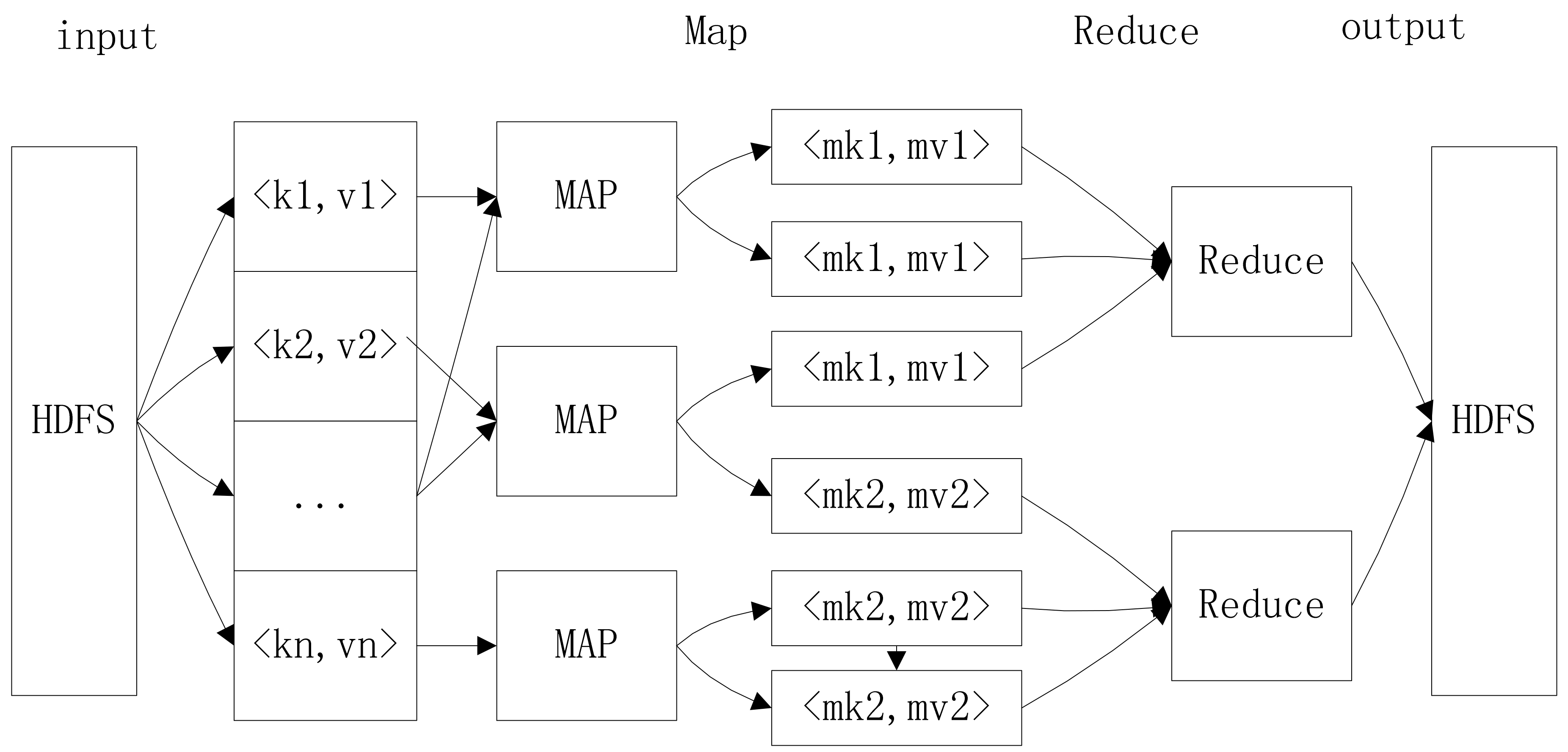
4.1. Map/Reduce Programming Model

Map/reduce is an extendable parallel programming model, which is widely used in the parallel computation of big data. The diagrammatic layout of map/reduce is shown in Figure 3.

Figure 3. Diagrammatic layout of map/reduce. MAP: the mapping process of hadoop; HDFS: hadoop distributed file system.

Map/reduce includes two phases: mapping and reducing. Every sub-process is highly parallel in these two phases. The specific procedures are as follows:

• The raw data are input into the key/value pairs (key, value), and the data are processed as much as possible without communication. The intermediate data created in map phase are also saved as key/value pairs (intermediate-key, intermediate-value).
• The intermediate pairs with the same intermediate-key are transferred to the same reducing process with the completion of the mapping process. The reducing process starts when all intermediate data are transferred. When both mapping and reducing processes are completed, the final results are achieved.

4.2. The Algorithm of Ultra-Short-Term WPP

The map/reduce model is widely used to process big data, however, a single map/reduce job only can complete simple jobs. To solve complex problems, the complex process is usually divided into some sub-processes, and the work is completed together with many map/reduce jobs. Due to the complexity of the ultra-short-term WPP, which is proposed in Section 3.2, the work is completed by five map/reduce jobs (see Algorithm 1).

Algorithm 1. Parallel Ultra-short-term wind power prediction based on Map/reduce.

Job 1: Reducing dimension of NWP matrix.

Map: The NWP matrix $M$ is separated into N sub-matrixes $M_i$, where i = 1, 2, …, N. Each sub-matrix $M_i$ is a reduced dimension based on the method in Section 3.2.

(1) Each map process reads sub-matrix $M_i$ of $M$.

(2) The intermediate data pairs $(0,‘i,X_i’)$ is achieved by reducing the data dimension of each sub-matrix $M_i$, according to Equation (8).

Reduce: The reducing dimension series $X$ is created by connecting in order all $X_i$, which are from map process.

(1) $X=\left\{\right\}$;

(2) For i = 1:N                 $X_i$ is added to the end of $X$;        end for

(3) Output $X$;

For the sake of convenience, $X_0$ is the reduced NWP data series during 2L hours, which consists of two equal parts, namely, the former L hours and the latter L hours. $X_0$ is removed from $X$, and the remainder of $X$ is divided into N sub-series, $X_1,X_2,\dots ,X_N$, where $\left|X_{\mathrm{i}}\right||\ge 8L$, the head of $X_1$ is the first node in X, and the head of $X_{i+1}$ is the (8L − 1)-th node of $X_i$ from the bottom, $i=1,2,\dots ,N-1$.

Job 2: Searching top k sub-series, which are the most similar to X0.

Map:

(1) Each map process reads the pairs $(i,<X_i,X_0>)$;

(2) For j = 1:||Xi|| − L % where ||Xi|| is the length of Xi [31].

(1) We compute the DTW between $X_0$ and $X_{ij}$, which is $X_i$’s sub-series including L elements and starting with the j-th element of Xi;

(2) The intermediate data are key/value pairs (i, ‘j, DTW’)

End for

Reduce:

(1) $k=({\displaystyle \sum _{k=1}^{i-1}\Vert X_i\Vert })+j$;

(2) $S_k=|\theta -DT{W}_{ij}|$;

(3) Output $(k,S_k)$.

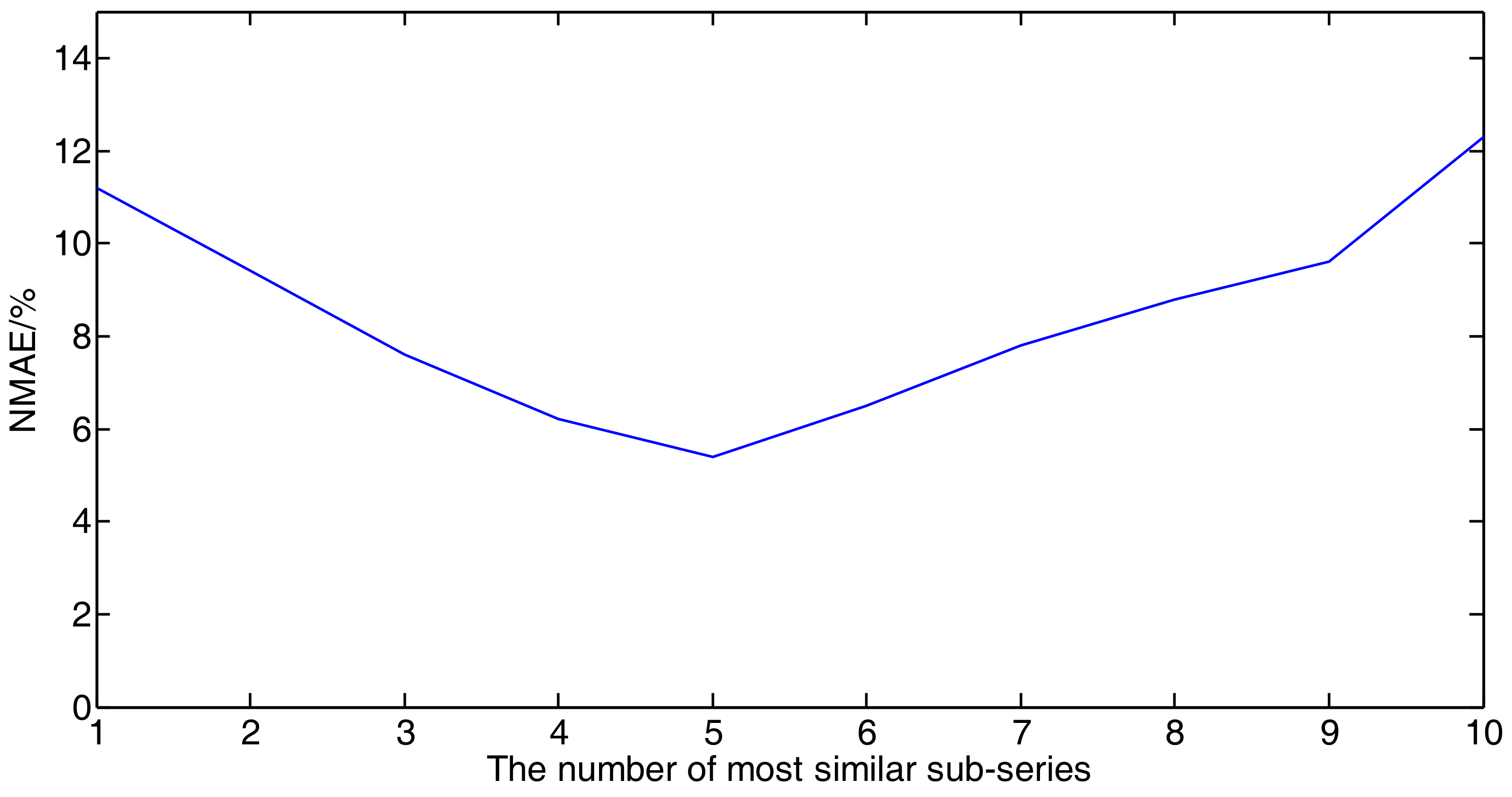
The sub-series are sorted by $S_k$ according to the method in reference [35], and the top k sub-series of NWP and wind power are selected. The top k most similar sub-series of NWP and wind power are denoted as $X_k$ and $P_k$, where k = 1, 2, …, k.

The sub-series are sorted by $S_k$ according to the method in reference [35], and the top k sub-series of NWP and wind power are selected. The top k most similar sub-series of NWP and wind power are denoted as $X_k$ and $P_k$ where k = 1, 2, …, k.

Job 3: The embedding dimension and delaying time of P and X are computed in this job.

For the sake of convenience, the time series P and X in our algorithm are denoted as P1 and P2, respectively.

Map:

(1) $(i,P_i)\stackrel{C-C a\lg orithm}{\to }(m_i,{\tau }_i)$;  % $m_i$ and ${\tau }_i$ are obtained by C-C algorithm

(2) $J_i=(m_i-1){\tau }_i$;         % calculating the starting index $J_i$ of Pi

(3) The intermediate data of this map are data pairs $(0,“m_i,{\tau }_i,J_i”)$, where $m_i$, ${\tau }_i$ and $J_i$ are the embedding dimension, delaying time, and starting point of Pi, respectively.

Reduce:

(1) J = $\underset{1\le i\le 2}{\max }\left\{J_i\right\}+1$

(2) $m_P=m_1,{\tau }_P={\tau }_1,m_X=m_2,{\tau }_X={\tau }_2$;

(3) Output $m_P,{\tau }_P,m_X,{\tau }_X,J$.

Job 4: Multivariate phase space reconstruction

Map:

(1) $(k,‘J\#m_X\#{\tau }_X\#m_P\#{\tau }_P\#X_k\#P_k’)\stackrel{reconstructed}{\to }(0,{\aleph }_k)$, where Xk and Pk are the most similar sub-series of top K achieved from Job 2, and $k=1,2,\dots ,k$.

Reduce:

(1) Output reconstructed phase space ${\aleph }_k$.

Job 5: Multi-variables linear regression

Map:

(1) Input $<i,‘{\aleph }_k\#S_k\#{\aleph }_0’>$, where ${\aleph }_0$ is the reconstructed phase space during 2L hours.

(2) The linear model is trained by $<{\aleph }_{k,j},{\aleph }_{k,j+1}$, where ${\aleph }_{k,j}$ is the j-th phase point of reconstructed phase space ${\aleph }_k$, j = 1, 2, …, $\Vert {\aleph }_k\Vert -1$;

(3) After the linear model has been trained, the next phase point is obtained according to Equation (12) and the last point of ${\aleph }_0$.

(4) The step 3 is executed iteratively, and then the forecasting reconstructed phase space ${\aleph }_k^P$ is achieved.

(5) The forecasting power sequence $P_{kj}$ is obtained based on an inverse process of the phase space reconstruction and reconstructed phase space ${\aleph }_k^P$.

(6) The intermediate data are $<0,‘P_{kj},S_k’>$.

Reduce:

The comprehensive wind power is given as follows.

$$P_j=\frac{S_k}{{\displaystyle \sum _{k=1}^k{S}_k}}{P}_{kj},k=1,2,\dots ,k;j=1,2,\dots ,B$$ (20)

where j = 1, 2, …, B, and B is the forecasting time-scale

5. Application and Case Study

5.1. The Experimental Data and Environments

The experimental data includes 2 sections: NWP data and wind power data. The NWP data ranged from 1 September 2012 to 31 August 2013 and were from the key laboratory of regional numerical weather predictions in a province of China. NWP data include temperature, humidity, wind speed, wind direction, atmosphere pressure, and so on. The NWP is from the mesoscale numerical prediction model. The temporal resolution of NWP is 1 h. The horizontal resolution of NWP is 3 × 3 km, and it is improved to 1 × 1 km by the dynamic downscaling model [36]. In our experiment, only the data of wind speed, wind direction, and atmosphere pressure were selected. The wind speed and wind direction were first converted into x components and y components, where the east and north are regarded as the positive direction of x-axis and y-axis, respectively. The converted NWP data are shown in Table 3.

Table 3. Historical numerical weather prediction (NWP) data of a wind farm.

No.	Time 1 February 2013	Wind Speed X-Direction (m/s)	Wind Speed Along Y Direction (m/s)	Atmosphere Pressure (atm)
1	1:00	7.43	6.45	0.98
2	2:00	8.6	5.36	0.98
3	3:00	6.07	9.05	0.986
…	…	…	…	…

In Table 3, each row is an NWP data record, which is composed of the time, the wind speed in the x-component, the wind speed in the y-component, and the atmosphere pressure. simple interpolation method was used to get the 15-min NWP data. The wind power (15-min) from 1 September 2012 to 31 August 2013 was used to train the model. The Figure 4 shows the daily peak wind power in each month.

Figure 4. Historical data of wind power.

In Figure 4, the x axis is time, y axis is the per-unit value of wind power. Because the wind power fluctuates severely at different times, the data are normalized based on Equation (18).

$$P_N=P/P_{\max }$$

(21)

where $P_N$ is the normalized wind power, $P$ is wind power, and $P_{\max }$ is the peak daily wind power from 1 September 2012 to 31 August 2013.

To implement the experiment, we tried to establish an experimental cloudy computing platform Hadoop, which is composed of five nodes including a 4-core central processing unit (CPU) (Intel Core i5) and an Ubuntu operation system. The ultra-short-term wind power was individually predicted by continuous prediction method, simple approximation method, and other methods proposed in this paper.

In terms of continuous prediction method, the nearest observed values were regarded as the next predicting values, namely $x_{i+1}^{\prime }=x_i$. The simple approximation method is another kind of continuous method based on phase space reconstruction, and the nearest observed phase points were regarded as the values of next phase point i, namely, $X_{i+1}^{\prime }=X_{j+1}$, where $X_j$ is the nearest phase point of $X_i$. The error index was the normal mean absolute error (NMAE) in this paper.

$$NMAE={\displaystyle \sum _{i=1}^N\frac{|x_i-y_i|}{N\times C}}$$

(22)

where $x_i$ is the measured wind power, $y_i$ is the forecasting wind power, C is the installed capacity of wind farm, and N is the number of periods being forecasted. More details about NMAE are described in reference [26].

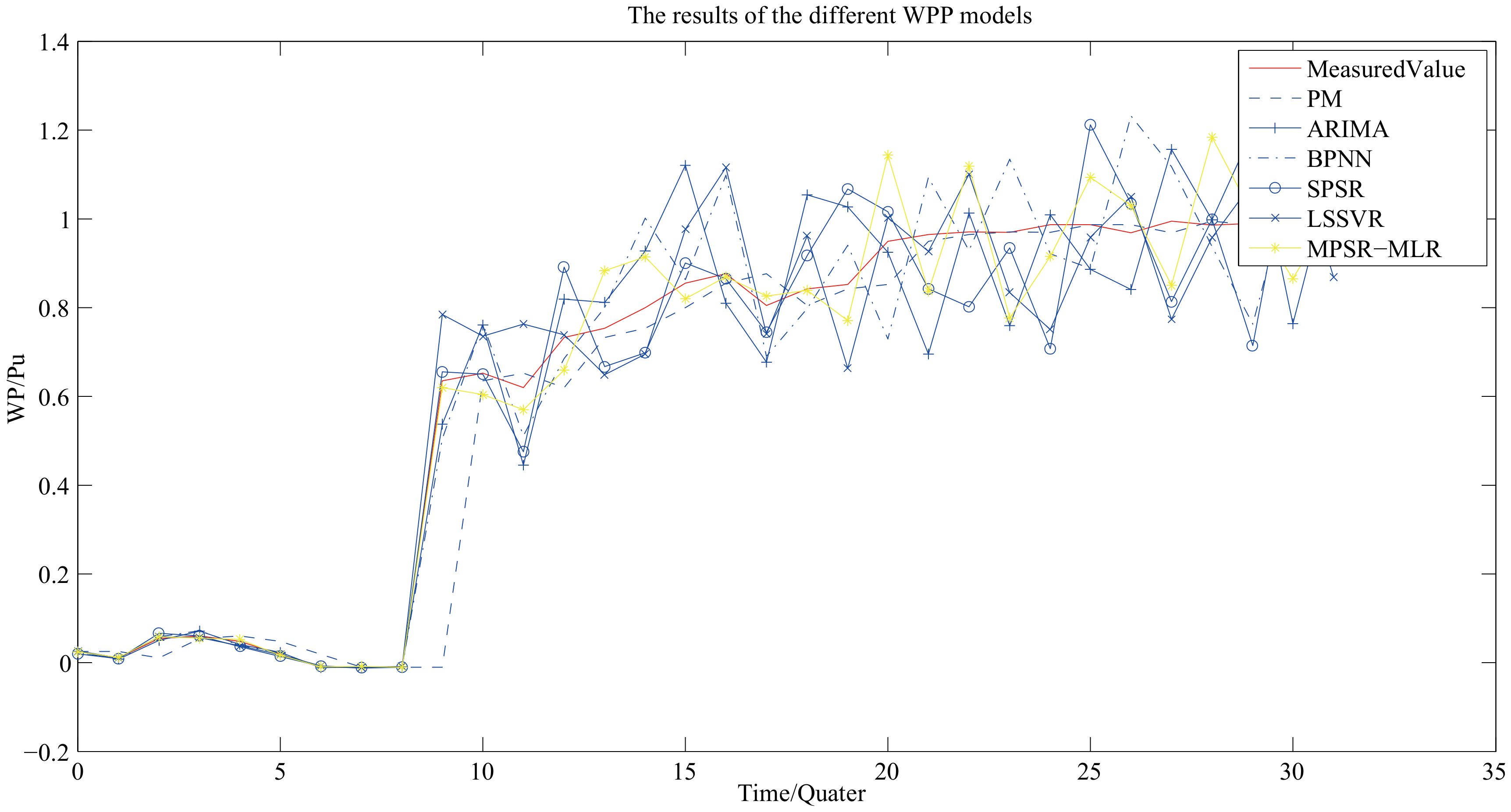
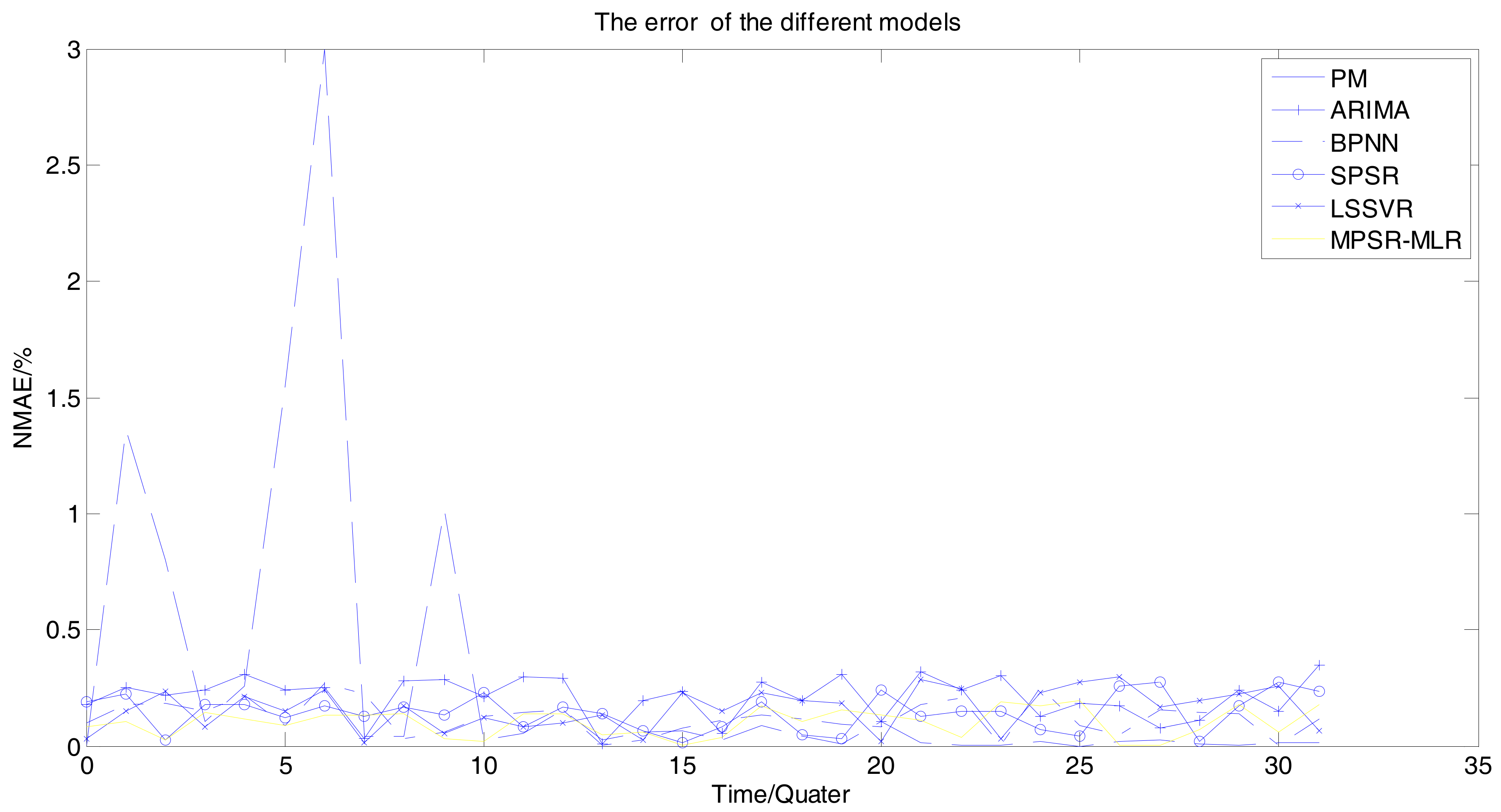
5.2. Results and Analysis of the Experiment

The embedding dimension and delaying time of wind power series P and NWP series X were computed by C-C method with 4000 points and 8000 points, respectively. The embedding dimension and delaying time of wind power series P were 5 and 18, respectively. The embedding dimension and delaying time of NWP series P were 6 and 17, respectively.

The number of the most similar sub-series could affect the ultra-short-term wind power prediction. To optimize the number of most similar sub-series, the number of most similar sub-series ranged from 1 to 10 in the experiment. The experimental results are shown as Figure 5, when the number of most similar sub-series ranges from 1 to 10.

Figure 5. Relation between the number of most similar sub-series and normal mean absolute error.

Figure 5 shows the relation between NMAE and the number of most similar sub-series. When fewer of the most similar segments (especially 1) are used to train a multi-variate linear regression model, the multi-time weighted linear regression becomes a single variable linear regression, and the results have bigger errors. With increasing K, the errors are slowly reduced. When K is near to the threshold, the NMAE keeps getting smaller. However, when the K is larger than a certain number, the errors increase slowly. The reason for this phenomenon is that the dissimilar series could increase the errors of ultra-short-term WPP. A good result can be achieved when K is between 4 and 8.

Figure 6 demonstrates the relation between forecasting time-scale and errors. When the predicting time-scale is less than 6 h, the predicting errors are stable and smaller. With an increasing forecasting time-scale, the average predicting error increases gradually. Figure 6 illustrates that the proposed model is suitable for ultra-short-term WPP, due to its smaller predicting time-scale.

Figure 6. Relation between time-scale and NMAE.

Our model is trained with the historical wind power and NWP data from 00:00 of 1 September 2012 to 24:00 of 31 August 2013. When the five most similar segments are used to train the linear regression model, the experimental results are shown in Figure 7.

Figure 7. Results of wind power predictions. ‘Measured Value’ is the measurement of wind power. ‘PM’ is the forecasting results of persistence method. ‘ARIMA’ is the forecasting results of the autoregressive integrated moving average. ‘BPNN’ is the forecasting result of the back propagation neural networks [37]. ‘SPSR’ is the forecasting of the WPP based on single-variable phase space reconstruction. ‘LSSVR’ is the forecasting results of the WPP based on LSSVR. ‘MPSR-MLR’ is the forecasting results of the proposed model.

Figure 7 shows that most of the forecasting results of the proposed model are near to the actual measurements. It proves that MPSR and MLR are suitable for ultra-short-term WPP. The error of the different models are shown as Figure 8.

Figure 8. The errors of different wind power predictions.

In Figure 8, ‘PM’ is the errors of the persistence method. ‘ARIMA’ is the errors of the WPP based on autoregressive integrated moving average. ’BPNN’ is the errors of the WPP based on back propagation neural networks [37]. ‘SPSR’ is the errors of the WPP based on the single-variable phase space reconstruction. ‘LSSVR’ is the errors of the WPP based on LSSVR. ‘MPSR-MLR’ is the errors of the proposed model. The statistical results of errors for different methods are listed in Table 4.

Table 4. Historical data of a wind farm.

No.	Methods	Max Error (%)	Min Error (%)	Avg Error (%)
1	PM	389.64	0.75	24.25
2	ARIMA	26.00	0.0114	12.76
3	BPNN	25.16	0.0089	10.40
4	LSSVR	21.24	0.0071	9.34
5	SPSR	22.36	0.0016	11.86
6	MPSR-MLR	14.38	0.0042	6.46

Figure 8 and Table 4 show that PM is not applicable to the seriously fluctuating wind power series. MPSR-MLR can reduce the predicting errors in the seriously fluctuating wind power series. The error of our model is lower than that of other WPP methods. MPSR-MLR outperforms SPSR by mining the correlation of different time series.

6. Conclusions

Various models and methods have been extensively employed in the field of ultra-short-term WPP as no model is suitable for all conditions and all wind farms. In order to improve the ultra-short-term WPP, we have proposed a novel model of the ultra-short-term WPP based on the multi-variates phase space reconstruction and the linear regression in this paper. The proposed model improves the ultra-short-term WPP by mining the correlation of different time series. The performance is particularly good, when the wind power series fluctuate seriously. A map/reduce-based parallel algorithm is implemented on a cloudy computing platform, Hadoop. The research results allow for three conclusions:

• Wind power is a chaotic time series, and multi-variate phase space reconstruction can improve the ultra-short-term WPP by mining the correlation of these wind power series.
• It is very difficult to forecast wind power, especially when the wind power series fluctuates seriously. The proposed model improves the performance during the wind ramp drastically.
• The forecasting speed is accelerated by adopting both the map/reduce-based parallel algorithm and the cloudy computing platform.

References

- Xue, Y.; Yu, C.; Zhao, J.; Li, K.; Liu, X.; Wu, Q.; Yang, G. A Review on Short-term and Ultra-short-term Wind Power Prediction. Autom. Electric Power Syst. 2015, 39, 141–151. [Google Scholar]
- Rafique, M.M.; Rehman, S.; Alam, M.M.; Alhems, L.M. Feasibility of a 100MW Installed CapacityWind Farm for Different Climatic Conditions. Energies 2018, 11, 2147. [Google Scholar] [CrossRef]
- Xie, W.; Zhang, P.; Chen, R.; Zhou, Z. A Nonparametric Bayesian Framework for Short-Term Wind Power Probabilistic Forecast. IEEE Trans. Power Syst. 2018. [Google Scholar] [CrossRef]
- Khorramdel, B.; Chung, C.Y.; Safari, N.; Price, G.C.D. A Fuzzy Adaptive Probabilistic Wind Power Prediction Framework Using Diffusion Kernel Density Estimators. IEEE Trans. Power Syst. 2018, 958–965. [Google Scholar] [CrossRef]
- Wang, Y.; Liao, W.; Chang, Y. Gated Recurrent Unit Network-Based Short-Term Photovoltaic Forecasting. Energies 2018, 11, 2163. [Google Scholar] [CrossRef]
- Foley, A.; Leahy, P.G.; Marvuglia, A.; McKeogh, E.J. Current methods and advances in forecasting of wind power generation. Renew. Energy 2012, 31, 1–8. [Google Scholar] [CrossRef]
- Khodayar, M.; Wang, J.; Manthouri, m. Interval Deep Generative Neural Network for Wind Speed Forecasting. IEEE Trans. Smart Grid 2018, 1–16. [Google Scholar] [CrossRef]
- Pimkumwong, N.; Wang, M.-S. Online Speed Estimation Using Artificial Neural Network for Speed Sensorless Direct Torque Control of Induction Motor based on Constant V/F Control Technique. Energies 2018, 11, 2176. [Google Scholar] [CrossRef]
- Lu, P.; Ye, L.; Sun, B.; Zhang, C.; Zhao, Y.; Teng, J. A New Hybrid Prediction Method of Ultra-Short-Term Wind Power Forecasting Based on EEMD-PE and LSSVM Optimized by the GSA. Energies 2018, 11, 697. [Google Scholar] [CrossRef]
- Ozkan, M.B.; Karagoz, P. A Novel Wind Power Forecast Model: Statistical Hybrid Wind Power Forecast Technique (SHWIP). IEEE Trans. Ind. Inform. 2015, 11, 375–387. [Google Scholar] [CrossRef]
- Shi, J.; Ding, Z.; Lee, W.-J.; Yang, Y.; Liu, Y.; Zhang, M. Hybrid Forecasting Model for Very-Short-Term Wind Power Forecasting Based on Grey Relational Analysis and Wind Speed Distribution Features. IEEE Trans. Smart Grid 2014, 5, 521–526. [Google Scholar] [CrossRef]
- Xu, Q.; He, D.; Zhang, N.; Kang, C.; Xia, Q.; Bai, J.; Huang, J. A Short-Term Wind Power Forecasting Approach with Adjustment of Numerical Weather Prediction Input by Data Mining. IEEE Trans. Sustain. Energy 2015, 6, 1283–1291. [Google Scholar] [CrossRef]
- Safari, N.; Chung, C.Y.; Price, G.C.D. Novel Multi-Step Short-Term Wind Power Prediction Framework Based on Chaotic Time Series Analysis and Singular Spectrum Analysis. IEEE Trans. Power Syst. 2018, 33, 590–601. [Google Scholar] [CrossRef]
- Lee, D.; Baldick, R. Short-Term Wind Power Ensemble Prediction Based on Gaussian Processes and Neural networks. IEEE Trans. Smart Grid 2014, 5, 501–510. [Google Scholar] [CrossRef]
- Chen, L.; Lai, X. Comparision between ARIMA and ANN models used in short-term wind speed forecasting. In Proceedings of the 2011 Asia-Pacific Power and Energy Engineering Conference, Wuhan, China, 25–28 March 2011; pp. 1–4. [Google Scholar]
- Zeng, J.; Qiao, W. Short-Term Wind Power Prediction Using a Wavelet Support Vector Machine. IEEE Trans. Sustain. Energy 2012, 3, 255–264. [Google Scholar] [CrossRef]
- Giorgi, M.G.D.; Campilongo, S.; Ficarella, A.; Congedo, P.M. Comparison between wind power prediction models based on wavelet decomposition with least-squares support vector machine (LSSVM) and artificial neural network (ANN). Energies 2014, 7, 5251–5272. [Google Scholar] [CrossRef]
- Wu, Q.; Peng, C. Wind power generation forecasting using least square support machine combined with ensemble empirical model decomposition, principal component analysis and a bat algorithm. Energies 2016, 9, 261. [Google Scholar] [CrossRef]
- An, X.L.; Jiang, D.X.; Zhao, M.H.; Liu, C. Short-term preciton of wind power using EMD and chaotic theory. Commun. Nonlinear Sci. Numer. Simul. 2012, 17, 1036–1042. [Google Scholar] [CrossRef]
- Zhang, Y.; Lu, J.; Meng, Y.; Yan, H.; Li, H. Wind power short-term forecasting Based on Empirical Mode Decomposition and Chaotic Phase Space Recontruction. Autom. Electric Power Syst. 2012, 36, 24–28. [Google Scholar]
- Yang, L.; He, M.; Zhang, J.; Vittal, V. Support-Vector-Machine-Enhanced Markov Model for Short-Term Wind Power Forecast. IEEE Trans. Sustain. Energy 2015, 6, 791–799. [Google Scholar] [CrossRef]
- Morshedizadeh, M.; Kordestani, M.; Carriveau, R.; Ting, D.S.-K.; Saif, M. Power production prediction of wind turbines using a fusion of MLP and ANFIS networks. IET Renew. Power Gener. 2018, 12, 1025–1033. [Google Scholar] [CrossRef]
- Rarki, R.; Thapa, S.; Billinto, R. A Simplified risk-based method for short-term wind power commitment. IEEE Trans. Sustain. Energy 2012, 3, 498–505. [Google Scholar]
- Wen, Y.; Li, W.; Hunag, G.; Liu, X. Frequency dynamaics constrained unit commitment with battery energy storage. IEEE Trans. Power Syst. 2016, 31, 5115–5125. [Google Scholar] [CrossRef]
- Bitaraf, H.; Rahman, S.; Pipattanasomporn, M. Sizing energy storage to mitigate wind power forecast error impacts by signal processing techniques. IEEE Trans. Sustain. Energy 2015, 6, 1457–1465. [Google Scholar] [CrossRef]
- Zhao, Y.; Ye, L.; Pinson, P.; Tang, Y.; Lu, P. Correlation-Constrained and Sparsity-Controlled Vector Autoregressive Model for Spatio-Temporal Wind Power Forecasting. IEEE Trans. Power Syst. 2018, 33, 5029–5040. [Google Scholar] [CrossRef]
- Cui, B.; Zhao, Z.; Tok, W.H. A Framework for similarity search of Time Series Cliques with Natural Relations. IEEE Trans. Knowl. Data Eng. 2012, 24, 385–398. [Google Scholar] [CrossRef]
- Schramm, R.; Jung, C.R.; Miranda, E.R. Dynamic Time Warping for Music Conducting Gestures Evaluation. IEEE Trans. Multimed. 2015, 17, 243–255. [Google Scholar] [CrossRef]
- Yin, H.; Yang, S.; Ma, S.; Liu, F.; Chen, Z. A novel parallel scheme for fast similarity search in large time series. China Commun. 2015, 12, 129–140. [Google Scholar] [CrossRef]
- Han, M.; Zhang, R.; Qiu, T. Multivariate Chaotic Time Series Prediction Based on Improved Grey Relational Analysis. IEEE Trans. Syst. Man Cybern. Syst. 2018, 1–11. [Google Scholar] [CrossRef]
- Mercorelli, P. Denoising and Harmonic Detection Using Nonorthogonal Wavelet Packets in Industrial Applications. J. Syst. Sci. Complex. 2007, 20, 325–343. [Google Scholar] [CrossRef]
- Johnson, M.T.; Povinelli, R.J.; Lindgren, A.C.; Ye, J.; Liu, X.; Indrebo, K.M. Time-domain isolated phoneme classification using reconstructed phase spaces. IEEE Trans. Speech Audio Proc. 2005, 13, 458–466. [Google Scholar] [CrossRef]
- Zhao, F.; Sun, B.; Zhang, C. Cooling, Heating and Electrical Load Forecasting Method for CCHP System Based on Multivariate Phase Space Reconstruction and Kalman Filter. Proc. CSEE 2016, 36, 399–406. [Google Scholar]
- Jin, J. Research on Optimization of Sorting Algorithm under MapReduce. Comput. Sci. 2014, 41, 155–159. [Google Scholar]
- Chen, N.; Qian, Z.; Nabney, I.T.; Meng, X. Wind Power Forecasts Using Gaussian Processes and Numerical Weather Prediction. IEEE Trans Power Syst. 2014, 29, 656–665. [Google Scholar] [CrossRef]
- Han, Y. The Design and Implementation of a Wind Power Forecasting System for Wind Farm in Gansu Province; University of Electronic Science and Technology of China: Chengdu, China, 2017. [Google Scholar]
- Castellani, F.; Astolfi, D.; Mana, M.; Burlando, M.; Meißner, C.; Piccioni, E. Wind power forecasting techniques in complex terrain: ANN vs. ANN-CFD hybrid approach. J. Phys. Conf. Ser. 2016, 735, 082002. [Google Scholar] [CrossRef]