1. Introduction
Voltage unbalance as a power quality (PQ) concern refers to the asymmetry of voltage magnitude or phase angle at the fundamental frequency between the phases of a three-phase power system. Due to the increased magnitude of single-phase loads and unbalanced three-phase loads, voltage unbalance in the power system is actually increasing [
1]. For example, in a 10 kV distribution system in China, the ratio of three-phase unbalanced loads in this system accounted for 6.94% [
2]. Jouanne et al. [
3] showed that in a U.S. distribution system, approximately 30% of these buses have a voltage unbalance factor (
VUF) in the range of 1% to 3%. Asymmetrical supply voltage can result in many adverse effects on equipment and on the power system, which is intensified by the fact that a small unbalance in the phase voltage can cause a disproportionately larger unbalance in the phase current [
4]. Nowadays, the unbalance problem has gained lots of attention from utility companies and customers [
3,
5]. For example, Bollen [
6], Kim et al. [
7], Chindris et al. [
8] and Ghijselen and Van den Bossche [
9] studied the definition, generating mechanism, standards, propagation and mitigation measures for the voltage unbalance. In 2008, the International Electro-Technical Commission (IEC) published a technical report that stipulates the unbalance emission limits for loads when they are connected to the high voltage, medium voltage and low voltage systems [
10]. On the other hand, when the point of evaluation (POE) voltage exceeds the specified limit, identifying the proportion at which each agent contributes to the unbalance becomes a necessary prerequisite for the targeted implementation of mitigation measures.
Compared with other PQ problems, such as harmonics and voltage sags [
11,
12,
13], research on the responsibility identification of voltage unbalance is relatively scarce [
14]. One of the first studies on the unbalanced source identification is based on the concept of conforming and nonconforming currents, which aims at the determination of responsibility for all PQ problems [
15]. The IEC/TR 61000-3-13-2008 technical report proposed a method based on the measurement of
VUF at POE pre and post the load connection [
10]. However, the need for identifying the impedances of transmission lines and evaluating the system pre and post the load connection limits the application of the method. Recently, Jayatunga et al. [
16,
17] have made improvements to the aforementioned method based on the availability of detailed parameters of the system. However, in the practical system, some parameters cannot be easily acquired. In 2010, a method based on the three-phase power flow was proposed to identify the contribution of a load or an unbalanced voltage source at POE [
18]. In this method, however, there is no mathematical model to permit assessing the significance of the negative sequence active power [
14,
19]. In summary, though the above research has promoted the development of identifying contribution of the power system three-phase unbalance, new methods still need to be developed in this area.
In particular, there are usually multiple feeders connected to the POE in the power system, and each feeder may supply energy for many loads, including balanced and unbalanced ones. When the POE bus voltage exceeds the unbalanced limit, it is quite meaningful to distinguish the individual contribution of the multiple unbalanced sources connected to the feeders. However, to the best of our knowledge, there is no research analyzing this problem. Therefore, in this paper, a two-step procedure is proposed to determine the unbalance contribution of the feeders connected to POE. The first step is to determine whether the main unbalanced source is at the upstream or downstream side of POE. If the main unbalanced source is located at the POE downstream, then the individual contribution of the unbalanced source connected to each feeder will be further assessed according to the second step. Moreover, a method is also proposed to estimate the equivalent negative sequence impedance of the aggregate loads connected to each feeder, and the impedance will be used for the contribution estimation.
The contents of the paper are organized as follows.
Section 2 establishes the equivalent circuit for the unbalance analysis and proposes the contribution estimation method. In
Section 3, the estimation process of the equivalent negative sequence impedance for the aggregate loads is illustrated.
Section 4 summarizes the detailed steps of the proposed method; and
Section 5 shows the simulation and field data analysis results. Finally, the conclusions of the paper are summarized in
Section 6.
2. The Proposed Unbalance Contribution Determination Method
Under normal operating conditions, the unbalanced voltage in the power system is principally caused by both structural and operational factors. Structural unbalance usually occurs due to incomplete transposition of transmission lines, asymmetrical wiring distribution of transformers, open-delta or open-Y-open-delta connected transformers, capacitor banks, aged fuses, etc. Operational unbalance can be considerable when single-phase and two-phase loads as well as any unbalanced three-phase loads, such as arc-furnaces, are supplied by the distribution network. Usually, the voltage unbalance at the POE is the collective effects of all the above unbalanced sources.
In the following section, a two-step procedure will be illustrated to identify the unbalance contribution of the multiple unbalanced sources at POE. First, whether the main unbalanced source is at the upstream or downstream side of POE is determined; then the unbalance contributions of the multiple unbalanced sources connected to the POE are analyzed. In the following discussion, the side determination of the main unbalanced polluter at the POE is called “single-point unbalanced source” problem, and the contribution determination of multiple unbalanced sources connected to the same bus is called the “concentrated-multiple unbalanced source” problem. Negative sequence is used to illustrate the method due to the negligible amplitude of zero sequence voltage in the three-phase three-wire system.
2.1. Contribution Determination for Single-Point Unbalanced Source Problem
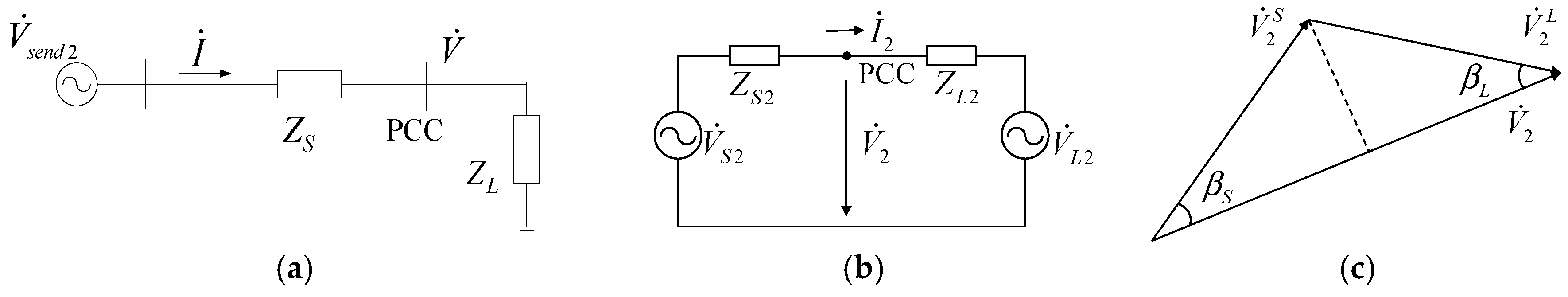
The analysis circuit for the single-point unbalanced source problem is shown in
Figure 1a. The unbalanced sources at the upstream network of POE may include the incomplete/untransposed transmission lines, the asymmetrical wiring of transformers, some unbalanced loads or equipment. The voltage unbalance caused by the upstream network is called the “background unbalance”, and is represented as
. The upstream system equivalent impedance seen from the POE is stipulated as
, which is shown in Equation (1):
ZSi (
i = 0, 1, 2) is the self sequence impedance, and
ZSij (
i = 0, 1, 2, and
j = 0, 1, 2) is the mutual impedance. The POE phase voltage and current can be measured and decomposed into their symmetrical components:
and
. In
Figure 1a,
represents the equivalent impedance of the downstream system, which has a similar form as
ZS.
Based on the upstream parameters, the negative sequence voltage of POE (
) can be expressed as follows:
The upstream background unbalance and the unbalance from the upstream asymmetrical impedance can be represented by voltage source
:
The unbalance voltage of POE can also be expressed in terms of the downstream parameters:
where
ZLi (
i = 0, 1, 2) and
ZLij (
i = 0, 1, 2, and
j = 0, 1, 2) are the equivalent sequence impedance and mutual impedances for the downstream network. Similarly, the voltage unbalance caused by the downstream sources can also be represented by an equivalent voltage source
:
Based on the above analysis, the Thevenin equivalent circuit for unbalance study can be established, as shown in
Figure 1b. The POE negative sequence voltage can be calculated according to the superposition theory:
where
denotes the POE negative sequence voltage contributed by the downstream unbalanced sources and
represents the negative sequence voltage resulted from the upstream source. Based on
Figure 1b, the POE negative sequence voltage
can also be calculated by Equation (7):
In the actual power system, the POE upstream equivalent impedance is mainly determined by the system short circuit impedance and the last transformer impedance. Usually, the upstream equivalent impedance is much smaller compared with the downstream impedance, which is mainly determined by the loads. Therefore, by simplifying Equations (6) and (7), the unbalance voltage produced by the upstream and downstream sources can be calculated according to Equation (8):
According to [
20], the voltage unbalance is defined as the ratio of the magnitude of negative-sequence voltage to the magnitude of the positive-sequence voltage, expressed as a percentage, which is notified as
VUF here:
Similar to the harmonic problem, the unbalance impacts can be quantified by the voltage projections, as shown in
Figure 1c, where
is the angle displacement between
and
,
is the angle displacement between
and
. Therefore, the unbalance indices to evaluate the unbalance contribution can be calculated based on the vector projections as shown in Equation (10).
UIS is the unbalance index for the upstream unbalanced source and
UIL is the index for the downstream source.
VUF is the simplification for the Voltage Unbalance Factor.
Based on the results of Equation (10), contributions of the upstream and downstream unbalanced sources can be compared and the main unbalanced polluter at the POE can be identified. If the main unbalanced source is determined to be at the upstream side, then mitigation measures should be targeted to the POE upstream. On the other hand, if the POE downstream is found to contain the main unbalanced source, then the individual unbalance contributions for the multiple feeders connected to the POE should be further estimated to locate the feeder with the most serious unbalanced load.
2.2. Contribution Determination for Concentrated-Multiple Unbalanced Source System
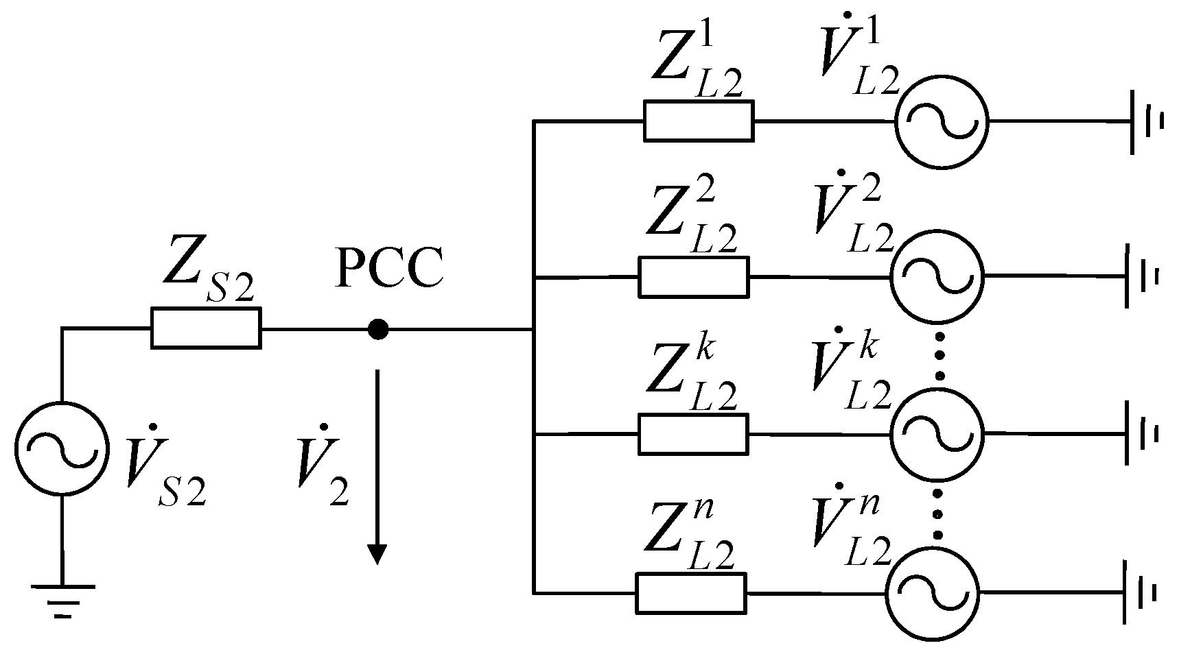
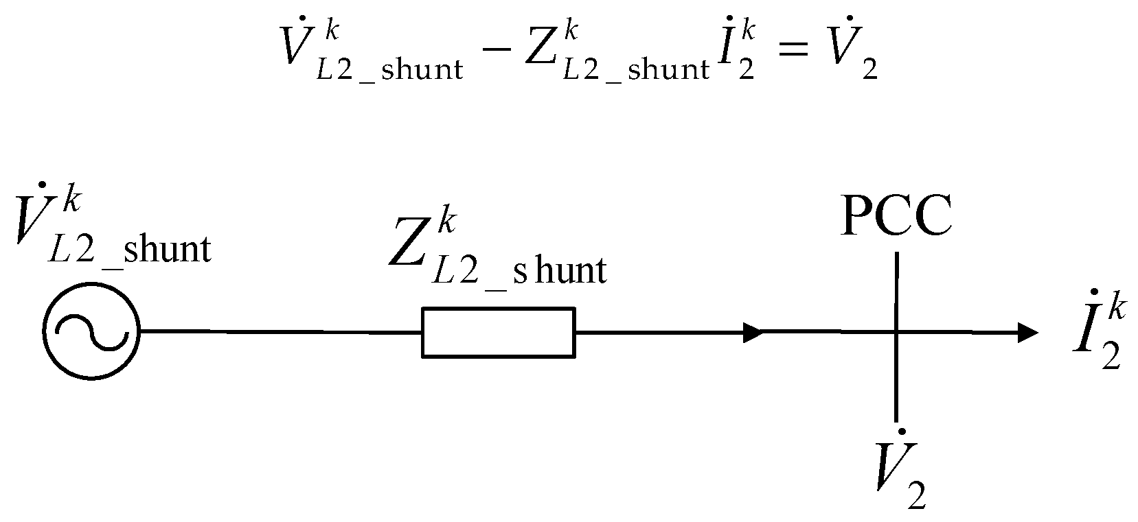
The analysis circuit for the concentrated-multiple unbalanced source system is shown in
Figure 2. The superscript of the variable denotes the index of feeder. For example,
is the negative sequence equivalent voltage source for load feeder
k, where
k = 1, 2, …,
n,
n is the total number of feeders. The unbalance voltage caused by the load on feeder
k is calculated based on Equation (11):
where
is the shunt impedance for all other branches except for feeder
k and it can be calculated by:
Similarly, based on the superposition theorem, the negative sequence voltage
at POE is caused by both the upstream unbalanced source and downstream unbalanced source from all feeders.
represents the equivalent unbalanced source of the upstream system and
is caused by the unbalanced loads in feeder
k. The contribution of
kth unbalanced source on the POE negative sequence voltage can be calculated by the projection of
on
; therefore, the unbalance index
can be calculated as below:
where
is the phase displacement between
and
,
k {
S; 1,2,3,…,
n}, here “
S” represents the system. From
Figure 2, it can be seen that the negative sequence current that resulted from the
kth unbalanced source is calculated by:
This negative sequence current is emitted by the unbalanced source in feeder
k individually, so it is named as the “individual current”. The POE unbalance voltage resulted from the source in feeder
k is calculated by the following:
Substituting Equation (16) into Equation (14), the unbalance contribution index
UIk can be calculated based on the “individual current”.
Actually, based on the Kirhoff’s current law, the unbalance current flowing in feeder
k is the collective effect of all unbalanced sources in the system, and it can be calculated according to Equation (18):
and
are the unbalance current caused by the upstream system and the unbalanced source on feeder
i, respectively,
i = 1, 2, ...,
n,
i ≠
k.
and
are shown below:
where:
Here, is the actual current flowing in feeder k, which is generated by all unbalanced sources in the system and can be measured from feeder k.
Based on the above analysis, it is known that the “individual current” is the real negative sequence current emitted by the objective unbalanced source, while the “actual current” is the current actually flowing in the branch, which is the superposition result of all unbalanced sources in the system. The “individual current” is accurate in representing the unbalanced source contribution; however, this current is difficult to obtain, while the “actual current” flowing in the feeder can be easily measured. Therefore, it is proposed to use the “actual current” to evaluate the unbalance contribution. Thus, the unbalance index can be modified as follow:
where
is the phase displacement between
and
.
2.3. Relationship Analysis between “Individual Current” and “Actual Current”
In this section, the feasibility of substituting the “actual current” for “individual current” in evaluating the unbalance contribution is verified. According to Equation (18), the difference between “actual current” and “individual current” is affected by both the load impedance and the equivalent unbalanced voltage source. The equivalent voltage source represents the unbalance level of the corresponding unbalanced source, while the impedance represents the load level. Therefore, in the following analysis, both the impedances and voltage source amplitudes are varied, trying to imitate enough fluctuation situations.
The concentrated three-feeder unbalanced source system in
Figure 2 is used as an example for illustration. The initial parameter values of the system are given in
Table 1. In the study, the loads are represented by impedance
Zi (
i = 1, 2, 3). The impedance value of feeder 1 is used as the basis, and the ratios of
Z2 to
Z1,
Z3 to
Z1 are defined as
Z21,
Z31, respectively. Different impedance combinations represent different load levels. The sub-cases of the impedance variation combinations are shown in
Table 2. On the other hand, the parameter variations for the voltage source are shown in
Table 3. Unbalance levels for both the feeders and the upstream source are varied randomly hundreds of times for each sub-case. Numerous simulation results have been obtained. However, due to the space limit, only the results for one sub-case are given here.
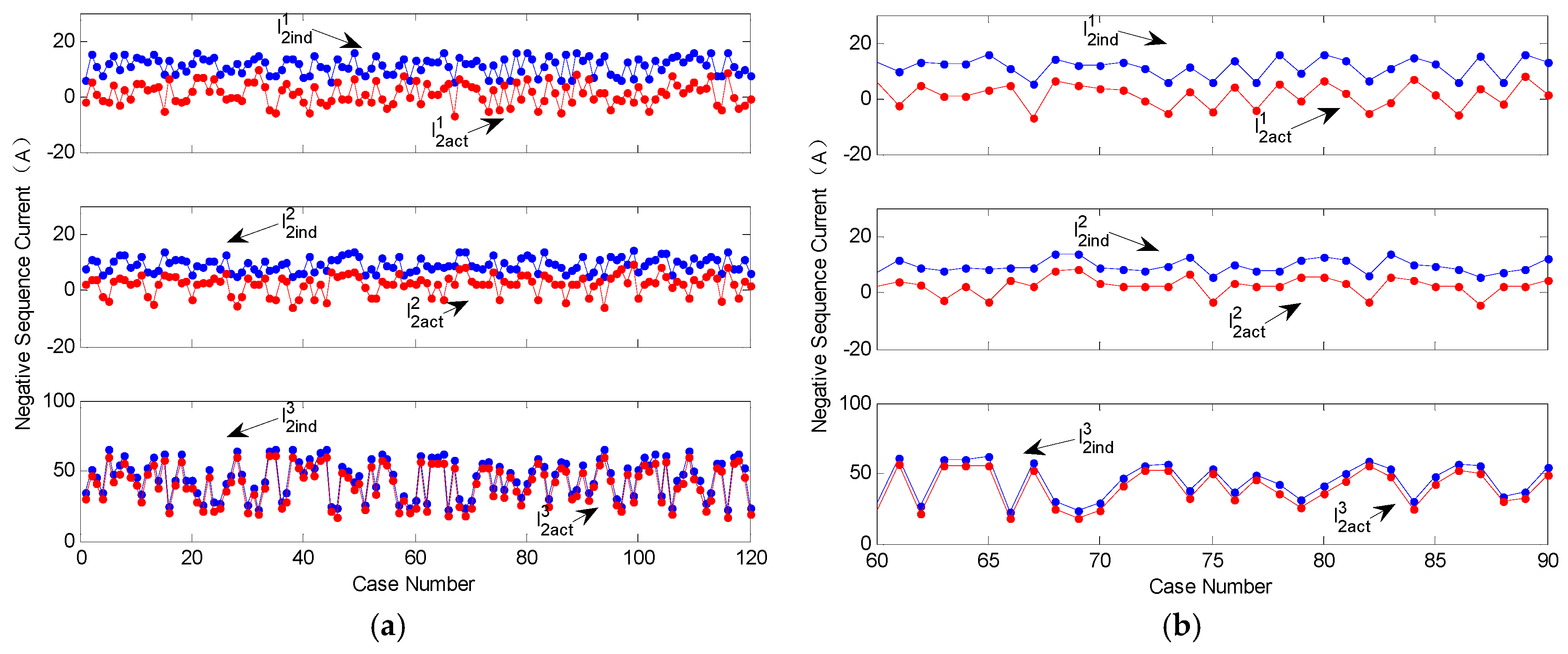
The variations of negative sequence “individual current” and “actual current” for each feeder are shown in
Figure 3a. In order to observe the relationships more clearly, results for cases 61–90 are enlarged as shown in
Figure 3b. From the results, it can be seen that the variation trends of the “individual current” and “actual current” are consistent with each other for all feeders. Therefore, it is proposed to use the “actual current” to estimate the unbalance contribution instead of the “individual current”.
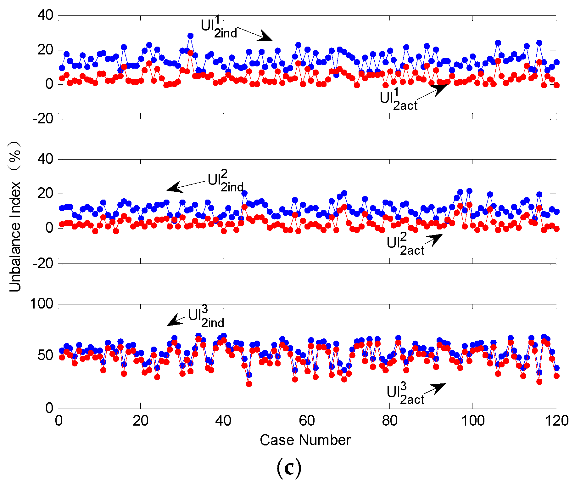
Figure 3c further shows the contribution estimation results based on the “individual current” and “actual current”. The estimation error (
EE) introduced by using the “actual current” to substitute the “individual current” is below 6% for all three feeders. The sensitivity of the estimation accuracy will be further discussed in the simulation part of next section.
3. Negative Sequence Shunt Impedance Estimation
From Equation (21), it is known that four parameters should be known before estimating the unbalance contribution for the unbalanced source connected to feeder k. The POE voltage and current flowing in feeder k can be directly measured, then, their negative sequence components and can be obtained based on the symmetric-component transformation. The equivalent impedance can be estimated based on the measured voltage and current data using the method proposed in this section. Then, the phase angle can be calculated based on the known impedance .
The power system seen from feeder
k can be modeled by a Thevenin equivalent circuit as shown in
Figure 4 [
21]. Here,
and
are the equivalent negative sequence voltage source and equivalent impedance for the other system except for feeder
k.
is the POE negative sequence voltage and
is the negative sequence current flowing in feeder
k. Based on
Figure 4, Equation (22) can be obtained:
The POE voltage
and feeder
k current
can be measured directly. Therefore, the unknowns in Equation (22) are
and
. Based on the measured data for
n time instants,
n equations can be written according to Equation (23):
where
ti is the
ith sampling time instant,
and
are the POE voltage and current in feeder
k at the time instant
ti (
i = 1, 2, …,
n), respectively. The
n equations can be manipulated into a matrix form.
Equation (24) can be further simplified into a compact form:
where
,
, and
.
The unknown variable
X in Equation (25) can be estimated using the least-square method. The objective function can be expressed as follows:
The final estimation values of the negative sequence equivalent circuit parameters for the systems viewed from feeder
k can be obtained according to Equation (27):
Moreover, the parallel equivalent impedance viewed from all other feeders can also be estimated based on the similar procedure as illustrated above.
4. Main Steps and Flowchart of the Proposed Method
Based on the procedures illustrated in
Section 2 and
Section 3, the main steps of the proposed unbalance contribution determination method can be summarized as follows.
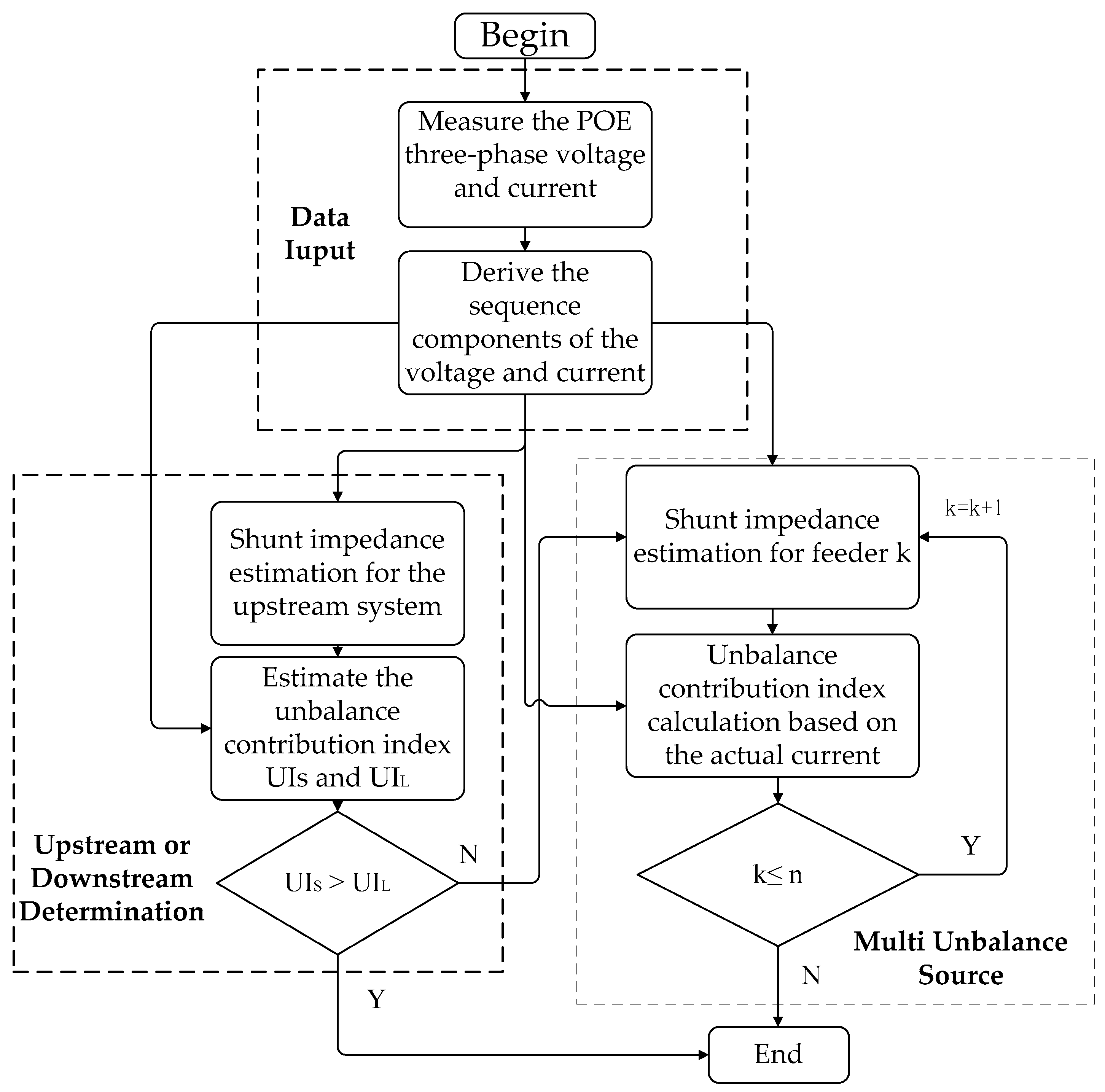
The first step is to measure the POE three-phase voltage and the currents flowing in each branch that connected to the POE. Discrete Fourier analysis is applied to the measured data in order to extract the fundamental frequency components. Then the phase-domain components of the voltage and current are transformed into sequence-domain components by means of the symmetric-component transformation.
The second step is to determine whether the main unbalanced source is at the upstream or downstream side of POE. The negative sequence equivalent impedance of the upstream system can be estimated according to Equation (27). Then, the upstream unbalance contribution index UIS and downstream unbalance contribution index UIL can be calculated according to Equations (6)–(10). By comparing the unbalance contribution results, the main unbalanced source can be identified. If the main unbalanced source is determined to be located upstream of POE, the mitigation measures should be targeted to the upstream unbalanced sources. If the main unbalanced source is at the downstream of POE, the individual unbalance contribution for the multiple sources connected at the POE should be further determined based on the third step.
In the third step, the shunt parallel impedance for feeder k (k = 1, 2, …, n) can be first estimated according to Equation (27). Then the contribution of the unbalanced load on feeder k can be calculated according to Equation (21). This step should be repeated until the unbalance contributions for all n feeders have been estimated. Then the unbalance contribution of all sources can be determined according to the results.
The flowchart of the entire algorithm is presented in
Figure 5. The proposed method is mainly aimed for the “concentrated-multiple unbalanced source” problem, whereas it can also be individually applied to the “single-point unbalanced source” system, in which only the first two steps are needed.
5. Case Study Result Analysis
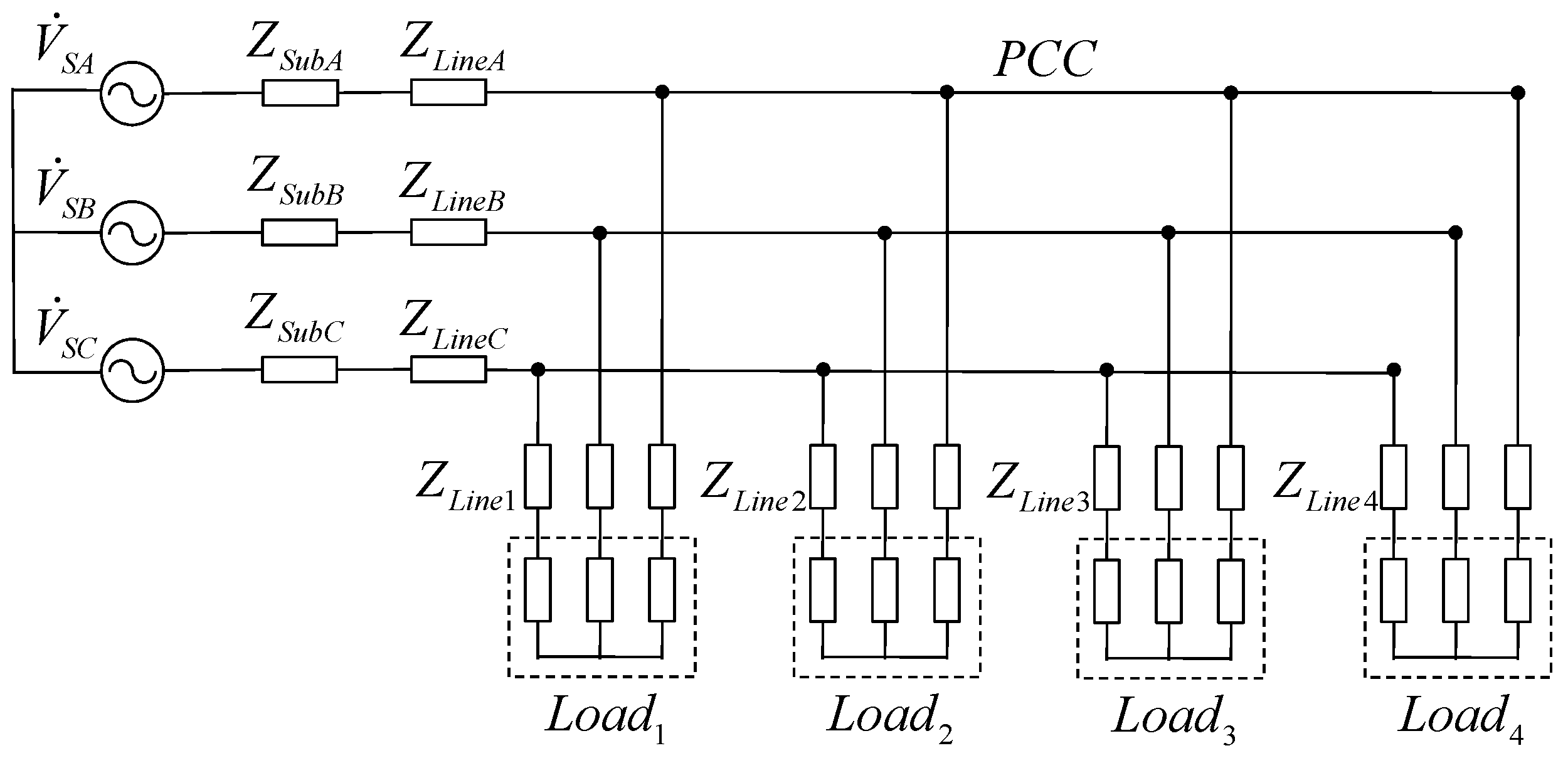
A 10 kV radial network is used to verify the proposed method. Single-line diagram of the system is shown in
Figure 6.
,
and
represent the system background unbalanced voltage.
,
and
are the upstream system equivalent impedances.
is the transmission line impedance. The detailed parameters for the test system are given below. The supply system equivalent impedances are
Zself = 0.4936 + 3.1026
j (Ω) and
Zmutual = −0.1976 + 0.1463
j (Ω). The transmission line is un-transposed and the impedance matrix per kilometer is:
The length of the transmission line is 2 km, and distribution line 1 is 6 km, line 2 is 8 km, line 3 is 5 km, and line 4 is 8 km. Loadi represents the unbalanced loads on feeder i. The rated load capacities for the four feeders are 0.8 MVA, 0.5 MVA, 0.6 MVA, and 0.1 MVA, respectively. The power factors for all loads are set to be 0.90. The unbalanced three-phase power flow was calculated based on the multiple-phase harmonic load flow (MHLF) program, and the results are used to validate the proposed method.
5.1. Negative Sequence Impedance Estimation
The loads of all feeders are randomly fluctuated within the range of 90% to 110% of their rated value. The supply system impedance parameters are changed at the time instants of
t = 10 s and
t = 20 s. For each time period, two thousand simulations have been implemented. Based on the procedure illustrated in
Section 3, the negative sequence impedance for the upstream system seen from the POE (
ZS2) and the parallel impedance for all other branches seen from feeder
k (
) are estimated. The estimation results are compared with their actual values as shown in
Table 4 (feeder 3 is used as an example). From the results, it can be observed that the estimated impedances have a good consistency with their exact values.
5.2. Unbalance Contribution Determination
Based on the procedure summarized in
Section 4, the contributions of all unbalanced sources are estimated by the proposed method. Three different cases have been used to verify the validity of the proposed method.
- Case 1:
Load of phase B on each feeder is set to 10% of its rated capacity, while loads of phase A and phase C take their rated capacities. The upstream three-phase voltage source is assumed to be ideally balanced.
- Case 2:
The load unbalance condition is the same as that in Case 1, while the voltage source of phase B at the upstream side of POE is set to
- Case 3:
The upstream unbalance condition is the same as that in Case 2. For the downstream side, the load of phase B changes to 70% SN, and loads of phase A and C take their rated value.
Table 5 shows the estimation results for the unbalance contribution. In the table, “accurate value” represents the contribution determination results obtained based on the superposition theory [
22], which is calculated by the MHLF program [
23]. “ICM” represents the results for the “individual current”-based method and “ACM” represents the results for the “actual current”-based method. It can be seen that, the “individual current”-based method is more accurate than the “actual current”-based method. The discrepancies between the “accurate value” and the two proposed methods are further calculated and shown in
Table 6. The
EE for the upstream unbalanced source is relatively large. This is because the unbalance emission level for the upstream unbalanced source is small, and the inherent law of the unbalanced current has been interfered by the unbalanced currents generated by other sources. The unbalance current generated by feeder 4 is much smaller than the upstream source, and it has been removed in the estimation procedure. Actually, such low emission unbalanced sources reduce the estimation accuracy of other feeders (details will be discussed in the next
Section 5.3).
In order to verify the accuracy of the proposed methods for more cases, one thousand scenarios were created by randomly varying the feeder impedances from 95% to 115% of their original values. The following estimation indices are defined in order to show the accuracy of the results in a more clear and compact way.
- (1)
Estimation Error
where
and
are the exact and estimated contribution indices for the unbalanced source.
- (2)
Average Accuracy (AA)
where
is the estimation error for the unbalanced source connected to feeder
k.
- (3)
Highest Accuracy (HA)
where
HA represents the highest estimation accuracy among all cases.
Based on the unbalance contribution estimation results, the above indices are calculated and shown in
Table 7. It can be observed that the highest accuracies of the two methods are both above 93%. The
AA of the “ICM” is above 89% and “ACM” is above 85%. Thus, the “actual current” can estimate the unbalance contribution with an acceptable accuracy. Since the “actual current” is easy to be measured from the feeders, while the “individual current” is difficult to obtain, it is more convenient to use the “actual current” in the unbalance contribution estimation.
5.3. Sensitivity Analysis
In this section, the performance of the method by using the “individual current” and “actual current” is compared. By varying the load unbalance degree in the multiple unbalanced source system, lots of simulation scenarios have been generated. The four-feeder system is used as an example to illustrate the method.
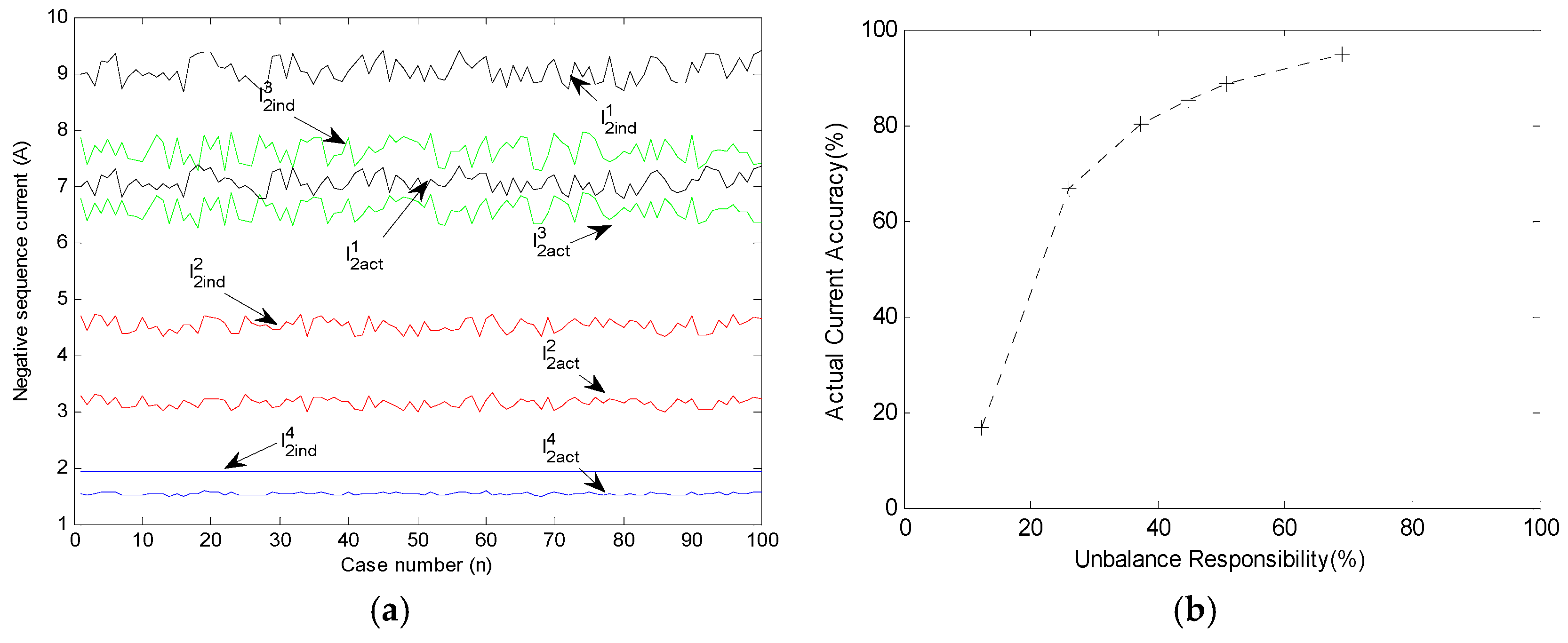
Figure 7a shows the variations of the “individual current” and “actual current” for different cases. It can be found that the variation trends of the “individual current” and “actual current” are consistent for feeders 1, 2, and 3. However, for feeder 4, there is no such a consistency. Coefficient
ACC is defined to evaluate the accuracy of using the “actual current” for estimation compared with using the “individual current”.
It can be seen that the value of
ACC is smaller than 1. As
ACC approaches 1, the “actual current” will be closer to the “individual current”, and the estimation accuracy will be improved by using the “actual current” to substitute the “individual current”. Based on the results shown in
Figure 7b, it can be found that, the
ACC values increase with the increment of the unbalance responsibility, which means that the unbalance estimation accuracy by using the “actual current” increases when the unbalanced source emission level gets higher.
Further simulation case study results also show that, when the unbalance emission level of the unbalanced source is low, the consistency between the “actual current” and “individual current” will not be as good as before. This inconsistency is because the background unbalance current has changed the inherent variation law of the unbalanced current generated by this load. Therefore, the estimation accuracy will be reduced by using the “actual current” to substitute the “individual current”. Since the unbalance level is low, the unbalance contribution for the load on this feeder can be neglected. It has also been observed that the contribution estimation accuracy for other sources can be improved by neglecting the load with low unbalance emission level.
Table 8 shows the unbalance contribution estimation results based on the “individual current” and “actual current”. In Case 1, the system has four feeders, while in Case 2, feeder 4 is excluded. The results show that the existence of load 4 reduces the estimation accuracy of other unbalanced loads. When load 4 is excluded, the estimation accuracy of other sources can be improved by using the “actual current” for estimation.
5.4. Field Data Analysis
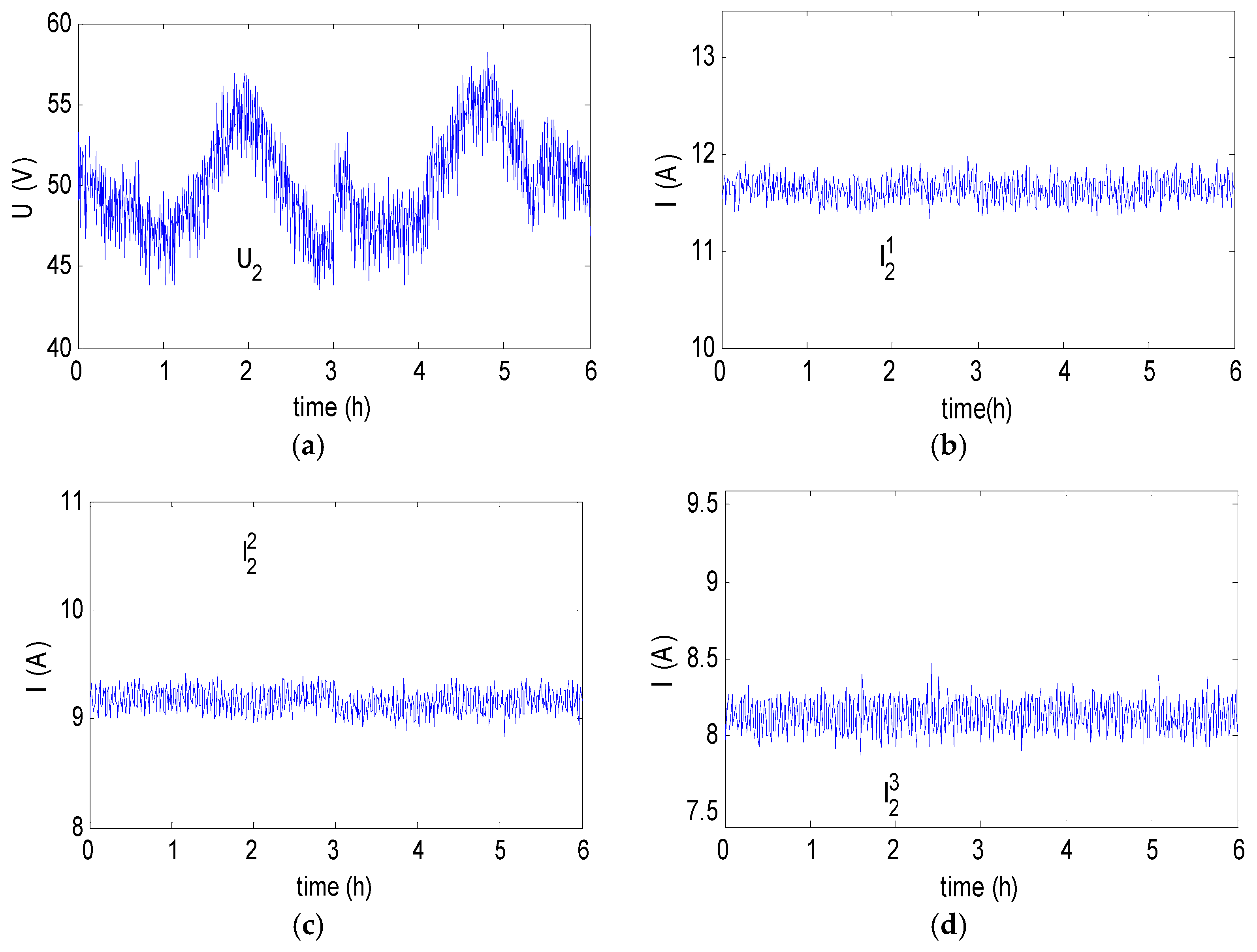
The proposed method has been applied to analyze the field data of a 10 kV substation that serves three load feeders. The national instrument NI-6020E 12-bit data acquisition system (NI-6020E, National Instruments, Austin, TX, USA) with a 12.8 kHz sampling rate was used for the data sampling, which can record 256 data points in each waveform. The measured waveforms are the three-phase voltage at the metering point and three-phase current flowing in each feeder. The measurements are taken as one snapshot per minute, while in every snapshot there are 10 cycle’s data recorded. Each cycle of the 50-Hz three-phase voltage and current waveforms are transformed into the frequency domain using discrete Fourier transform. The positive/negative sequence voltage and current for each cycle of the system frequency are calculated based on the sequence transformation matrix.
Figure 8 shows the root mean square (RMS) values of the negative sequence substation voltage and feeder current, where
h denotes hour. The average negative sequence
VUF is about 1.14%.
Based on the measured data, the equivalent shunt impedance seen from each feeder is estimated according to the method proposed in the paper, and the results are shown in
Table 9. The distribution system is then set up based on the estimated system parameters, and the unbalance contribution for each source is estimated according to the superposition method and the MHLF program. Moreover, the unbalance contribution is also estimated based on the proposed actual-current based method. From the results shown in
Table 10, it is known that the unbalance estimation results from the proposed method are generally consistent with the results from the superposition method (the accurate values). From the analysis in
Section 5.3, it is known that, if the unbalance emission level of a source is low, then the inherent variation law of its “actual current” will be interfered by other unbalance sources. Therefore, the contribution estimation accuracy of this source will be reduced. In this system, the unbalance emission level of the upstream is the lowest, so the unbalance contribution estimation accuracy of the upstream is lower than other sources. Actually, the results of this part are consistent with the conclusion drawn in
Section 5.3. The results also indicate that the unbalance mitigation measures should first be targeted to the two most severe unbalanced sources which are connected to feeders 1 and 2, whose unbalance contribution is estimated to be 39.13% and 27.66%, respectively.
6. Conclusions
This paper has analyzed the responsibility determination for the multiple unbalanced sources at the point of common coupling in the power system. The main contributions of the paper are summarized as follows:
First, a new method is proposed to identify the unbalance contribution of each unbalanced source connected at the POE, including the upstream unbalanced sources and the downstream multiple unbalanced sources.
Second, the paper proposed a method to estimate the negative sequence equivalent impedance for the system seen from each feeder at the POE.
Third, the current flowing in each load feeder (“actual current”) is proposed to be used for the unbalance contribution estimation instead of the current actually emitted by the unbalanced source (“individual current”).
It is found that, under most situations, the “individual current” and “actual current” share the same variation trend. Therefore, the “actual current” can be used for the unbalance responsibility determination with a good estimation accuracy. However, when the load unbalance emission level is low, it is better to neglect this load’s contribution and the estimation accuracy of other main unbalanced sources can be improved.
The proposed method is mainly focused on the “concentrated-multiple unbalanced source” problem, whereas it can also be applied to the “single-point unbalanced source” problem, in which the unbalance contributions for the system and customer need to be determined. The proposed method only needs the measured POE voltage and feeder currents as its input; therefore, it is convenient to be used in actual applications.


