Abstract
Current integration and co-movement among international stock markets has been boosted by increased globalization of the world economy, and profit-chasing capital surfing across borders. With a reputation as the fastest growing economy in the world, China’s stock market has continued gaining momentum during recent years and incurred growing attention from academicians, as well as practitioners. Taking into account economic and geographical considerations, the US and Hong Kong are considerably the most comparable stock markets to China. The usual vector error correction model (VECM) could overlook the long memory feature of cointegration residual series, which can in turn exert bias on the resulting inferences. To overcome its limitations, we employ a fractionally integrated VECM (FIVECM) in this paper to investigate the long-term cointegration relations binding China’s stock market to the aforementioned stock markets. In addition, by augmenting the FIVECM with multivariate GARCH model, the return transmission and volatility spillover between market return series were revealed simultaneously. Our empirical results show that China’s stock market is fractionally cointegrated with the two markets, and it appears that China’s stock market has stronger ties with its neighboring Hong Kong market than with the world superpower, the US market.
1. INTRODUCTION
Globalization has been gaining momentum and has become irreversible regardless of sporadic oppositional influences. This phenomenon is a direct result of increased interaction between world economies, including both developing and developed countries. The stock market is one of the forefront players in this unprecedented spectacle in history, whilst the examination of integration within the world stock markets is one of the most important issues in finance.
A large number of studies have been examining integration among the world’s stock markets. In an era of increasing globalization where there is a substantial capital flows across countries, integration among world stock markets has important practical relevance for both investors and financial policy makers. An important determinant of interdependence among stock markets across countries is economic integration in the form of trade and investment flows. The dividend discount model suggests that the current share price equals the present value of future cash flows, which depends on the earnings growth of a company. On the other hand, earnings growth also depends on the macroeconomic conditions of the domestic market as well as the macroeconomic conditions in countries with which a country trades and sources its investment flows (Shamsuddin and Kim, 2003). Thus, interdependence in stock markets may also reflect geographical proximity among markets with economically close ties. They are expected to exhibit high levels of market linkages because of the presence of similar investor groups and cross-listed companies.
However, greater financial integration implies reduced opportunities for international portfolio diversification. Co-movements among markets can result in contagious effects where in an effort to form a complete information set, investors incorporate price changes in other markets into their trading decisions, inferring that shocks and errors in one market can be transmitted to other markets. Such contagious effects have been exacerbated by major events which have affected world stock indices in recent decades such as the 1987 stock market crash, Asian financial crisis in 1997, and the recent world financial crisis in 2008. Correspondingly, individual countries’ monetary and fiscal schemes are being designed to tackle possible external infections.
This paper focuses on examining relations between China’s stock market and world markets partially represented by the US and Hong Kong markets. We attempt to detect the relations between China and these two particular markets because these two markets are believed to have stronger relations with China than other markets in the world. The US market is the leading and most influential market in the world, it is also the largest trading partner of and the biggest foreign direct investment source for China. Hong Kong, on the other hand, is China’s closest market due to economic, political, and geographical factors. Interdependence in stock markets may also reflect geographical proximity between markets, like China and Hong Kong, whom have economically close ties which are expected to exhibit high levels of market linkages because of the presence of similar investor groups and cross-listed companies. Conclusions from the interactions of China’s stock market with the US and Hong Kong markets may depict the main topology of China’s market in the world, the former shows the hierarchical importance of the world’s superpower, and the latter exhibits a close neighbor in the evolution of China’s stock market. Inferences could be valuable to international portfolios coving these markets.
In addition, this paper makes a methodological contribution to extend the vector error correction model (VECM) to the fractionally integrated VECM (FIVECM) in examining the co-movements of the China’s market with the US and HK markets. Using FIVECM enables investors not only to reveal the existence of a long-run equilibrium relationship and short-run dynamics among cointegrated variables, it also accounts for possible long memory in the cointegration residual series which may otherwise bias the estimation and draw misleading inference. Furthermore, conditional heteroskedasticity is often observed in market return series due to ever-changing underlying economic conditions over time. Accordingly, we augment the FIVECM with a GARCH-type model to capture the second moment autocorrelations in the return series. In particular, we employ the BEKK(1,1) model proposed by Engle and Kroner (1995) to model the evolution of conditional variances. Since there are no restrictions1 imposed on the coefficient matrices of conditional mean and conditional variance equations, lead-lag relations in the return series and the possible volatility spillover effects are simultaneously revealed in this model.
Our empirical findings clearly demonstrate that China’s stock market is fractionally cointegrated with both US and Hong Kong markets. Though the volatility spillover between China and the US markets is not clear, in this paper we discovered information transmissions between China and Hong Kong markets. Overall, our empirical evidence demonstrates that China’s stock market has a closer relation with Hong Kong market than the US market. This finding reflects the fact that China’s stock market and financial market as a whole is still under-liberalized and regulated, which renders it operating relatively independent of world’s leading market. The close nexus between China’s and Hong Kong markets is also attributable to the strong dependency of the HK economy to mainland China. We further divided the sample into two sub-samples marked by the East Asian Financial Crisis in 1998 and the recent world financial crisis in 2008 to the financial integration, in order to study the possible structural breaks caused by the crises. However, the estimation results did not show much difference for the two sub-samples before and after the crisis. Therefore, we will skip the discussion of the results for the sub-periods and stick to one sample investigation.
2. LITERATURE REVIEW AND MOTIVATIONS
The basic tenant of portfolio theory is that international investors should diversify assets across countries, provided that returns to stocks across countries are not highly correlated. The seminal studies of market interdependence and portfolio diversification include Grubel (1968), Levy and Sarnat (1970), Ripley (1973), and Lessard (1974). These studies have investigated integration between developed markets, integration between emerging markets, and integration between one or more developed markets and several emerging markets.
Most of the early studies used correlation analysis to examine short-run linkages between markets. However since the beginning of the 1990s, several studies, of which Kasa (1992) is one of the earliest, have used cointegration methods to examine whether there are long-run benefits from international equity diversification. Whether stock markets are cointegrated carries important implications for portfolio diversification. Cointegration between markets imply that there is a common force, such as arbitrage activity, to bring the movements of stock markets together in the long run, inferring that testing for cointegration is a test of the level of arbitrage activity in the long-run. In theory, if stock markets are not cointegrated, arbitrage activity to bring the markets together in the long-run is zero, inferring that investors can potentially obtain long-run gains through international portfolio diversification (Masih and Masih, 1997, 1999). On the other hand, if the markets are cointegrated, the predictability of each stock market can be enhanced through using information contained in the other stock markets. In this situation, the potential for making supra-normal profits through international diversification in the cointegrated markets is limited in the long run. This is because supra-normal profits will be arbitraged away in the long-run and, in the absence of barriers or potential barriers generating country risk and exchange rate premiums, one would expect similar yields for financial assets of similar risk and liquidity irrespective of nationality or location (von Furstenberg and Jeon, 1989).
Granger (1986) suggests that cointegration between two prices reflects an inefficient market on the basis that if two prices share a common trend in the long run, this implies predictability of each price’s movement, which in turn indicates that one market may be affected by another. The more accepted view, however, is that cointegration does not necessarily imply anything about efficiency (Dwyer and Wallace, 1992). For example, Masih and Masih (2002) suggest that a market is inefficient only if by using the predictability, investors can earn risk-adjusted excess returns, but predictability itself does not necessarily say anything about risk-adjusted excess rates of return.
Most studies testing for long-run relationships between markets have typically used the method of cointegration pioneered by Engle and Granger (1987) and Johansen (1988). Fernandez and Sosvilla (2001, 2003) examined stock market integration between the Japanese market and Asia Pacific markets, and United States market and Latin American markets, respectively, using the Johansen (1988) and Gregory and Hansen (1996) approaches to cointegration and found more evidence of cointegration allowing for a structural shift in the cointegration vector. On the other hand, Siklos and Ng (2001) considered whether stock markets in the Asia-Pacific region were integrated with each other, and with the United States and Japan using the Gregory and Hansen (1996) approach to testing for cointegration, and found that the 1987 stock market crash and 1991 Gulf War were turning points in the degree of integration.
Other common approaches to analyze co-movement include VAR analysis and Bayesian approach. For example, using VAR analysis, Eun and Shim (1989) found evidence of co-movements between the United States stock market and other world equity markets. Investigating the dynamics of stock market returns of the US, Japan and Asia-Pacific stock markets, Cheung and Ng (1992) found that the United States market was a dominant global force from 1977 through 1988. However, not all research supports cointegration among international stock markets. Using Bayesian methods, Koop (1994) concluded that there are no common stochastic trends in stock prices across selected countries. Due to the significance of October 1987 crash of the US market, Lee and Kim (1994) examined and found that national stock markets became more integrated after the crash. Similarly, using a VAR and impulse response function analysis, Jeon and Von-Furstenberg (1990) showed a stronger co-movement among international stock indices after the 1987 crash. There is a large literature on integration among the Asia-Pacific markets or integration between major world equity markets and Asia-Pacific markets. For example, Ng (2002) and Daly (2003) examined market linkages between Southeast Asian stock markets. There are several studies which consider whether the Japanese and/or United States market is cointegrated with Asia-Pacific markets (Cheung and Mak, 1992; Chung and Liu, 1994; Pan et al. 1999; Johnson and Soenen, 2002).
When a set of variables are cointegrated, the well-known Granger representation theorem yields vector error correction model (hereafter VECM) as the proper model to incorporate both cointegration relation and short-run dynamics among cointegrated variables. Most of cointegration studies listed above employs VECM to reveal the relations between underlying variables. The key aspect of VECM is that cointegration residual or error which is supposed to be I(0) process exerts correction effect to the long-run dynamics of underlying series. Specifically, when cointegrated variables deviate from the long-run relation, the immediately past period cointegration error acts as a force to pull the drifting variable back toward the equilibrium. This adjustment mechanism is based on the key assumption that the cointegration error follows a stationary I(0) process. However, the cointegration error between economic and financial series has been found to exhibit long memory feature which is consistent with neither stationary I(0) nor nonstationary I(1) processes. This special stochastic process is termed I(d) process with d being fractional real number, see, for example, Baillie (1996). When the cointegration error follows I(d) process which is found to be case for this study, long history of lagged cointegration errors also have correction effect to the dynamics of cointegrated variables. FIVECM has been applied to optimizing dynamic hedging ratios in derivatives market, like Lien and Tse (1999), but rare in studies on cointegration of equity markets.
Since China’s market has a short history, the interactions and relations between China’s market and other world markets have not been extensively investigated. One exception is Huang et al (2000) who examined whether there is a long-run relationship between the stock markets of the United States, Japan and the South China Growth Triangle using the Gregory and Hansen (1996) method and found that the only markets among these which are cointegrated were Shanghai and Shenzhen. However, China’s stock market, initiated in early 1990s, has made a leaping progress during its only fifteen years’ presence, the total capitalization has reached US$464.29 billion, 1378 companies are listed and more than 72 million investors are registered across the country (as of date Feb. 2005). Today, China is widely considered the most promising developing market. China’s rising stock market echoes its fast-growing economy and its increasing interaction with the world in terms of trade. China’s GDP has more than tripled from 1993 to 2003, the total amount of foreign trade (imports plus exports) of China jumped from US$115 billion in 1991 to US$1100 billion in 2004. China’s astonishing economic achievements during the last two decades are largely attributed to open and market-oriented economic policies implemented from early 1980s. As China’s economy is increasingly integrated with the world economy, China has also stepped up reforms and liberalizations of its financial market. Especially prior to and after joining the WTO, China accelerated the deregulation in financial market, meaning a great deal of the previous restrictions imposed on financial markets were lifted. Within 3-5 years, China’s financial market will be completely open to foreign investors. International investment funds are also preparing to the fully take advantage of the lucrative opportunities offered by China’s market. It is worthwhile at this critical point to assess the integration of China’s stock market with the world market proxied by the US and Hong Kong markets in this paper. The resulting inferences could yield some valuable insights to investors as well as policy makers.
3. DATA AND METHODOLOGY
3.1. Data description
We employed weekly data for the period from January 1998 through May 2009, giving 595 observations, in our study. Downloaded from Datastream, the stock price indices are the Shanghai All Shares Index () for China2, Hangseng Index () for Hong Kong, and S&P 500 () for the United States. To avoid the ‘day-of-the-week effect’ which suggests that the stock market is more volatile on Mondays and Fridays, we use the Wednesday indices, readers may refer to Lo and MacKinlay (1988) and Chen, et al. (2008) for the details. The sample covers the whole history of the Chinese stock market up to the commencement of this study.
The normalized indices with starting value for each index is set to be 100 are displayed in Figure 1, revealing that the Shanghai All Shares index is more volatile than the other two indices. This is also confirmed by the summary statistics of the data shown in Table 1. From the table, we notice that the standard deviation for the Shanghai All Shares index is 0.389, higher than those of S&P 500 and Hangseng indices, revealing higher variability in the China’s stock market. The most striking feature of the S&P 500 index from the figure is its continuous growth from early 2003 through mid 2007 when it reached a peak and then fell due to the subprime crisis which triggered the global financial crisis in 2008. Compared with S&P 500, Shanghai and Hangseng indices exhibit more large short-lived ups and downs in our studying period.
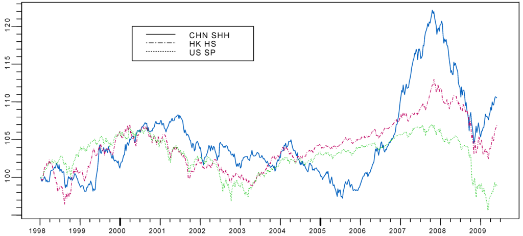
Figure 1.
Stock indices of China, USA and Hong Kong
Figure 1.
Stock indices of China, USA and Hong Kong
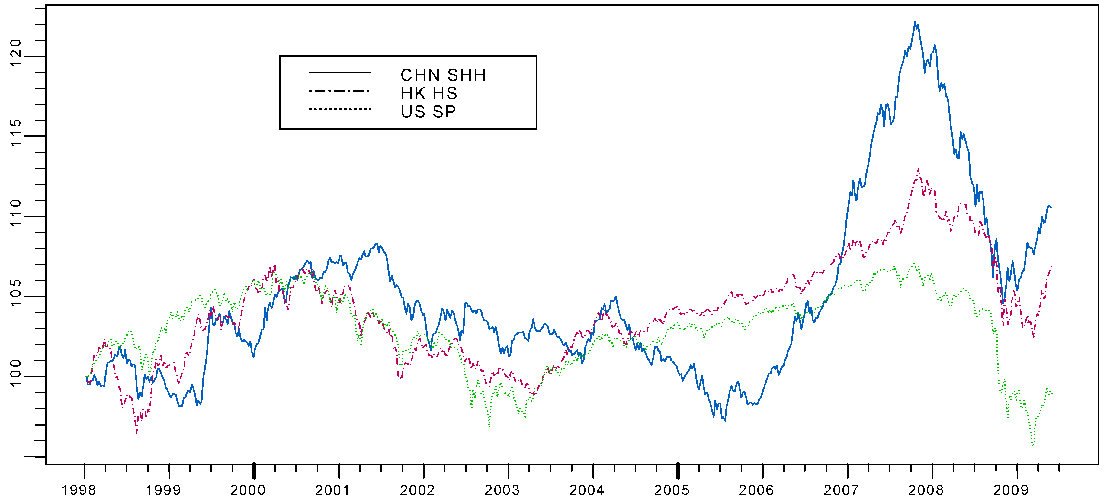
Notes : CHN SHH, HK HS, and US SP represent the normalized values of the Shanghai All Shares index, Hang Seng Index, and S&P 500, respectively. All indices are normalized so that they start at 100.

Table 1.
Descriptive statistics of data
| Statistics | SHHt | SPt | HSt |
|---|---|---|---|
| Min: | 6.928 | 6.569 | 8.833 |
| Mean: | 7.475 | 7.076 | 9.537 |
| Max: | 8.705 | 10.353 | 7.354 |
| Std Dev.: | 0.389 | 0.165 | 0.296 |
| Skewness: | 1.303 | -0.582 | 0.371 |
| Kurtosis: | 1.244 | -0.318 | -0.224 |
Notes: , , and are the logs of the weekly Shanghai All Shares index, Hangseng index, and S&P 500 index, respectively. The kurtosis is the excess kurtosis.
3.2: Methodology
To examine the existence of the cointegration relationship between stock price indices, we employ the Granger two-step procedure. In the first step, we fit the following dynamic ordinary least squares (DOLS) model to each pair of stock price indices:
Here, are the pair of stock indices chosen from , , and . Regression (1) is superior to the ordinary least squares, because the estimate from (1) is found by Stock and Watson (1993) to be super-consistent3 and asymptotically efficient. The estimated cointegration residual () can then be constructed by:
The definition of the cointegration approach suggests that some linear combinations of a set of I(1) variables could turn out to be stationary I(0) processes4. However, as first noted in early 1980’s, the characteristics of auto-dependence in cointegration residuals are found to comply with neither I(1) nor I(0) process. Baillie (1996) points out that the dichotomy between I(1) and I(0) could be too restrictive. Thereafter, researchers turn attention to investigate the process in the halfway between I(1) and I(0); that is, the fractionally integrated I(d) process with fractional real number d . In econometrics, the focus of study is on the I(d) process with -0.5<d<0.5, which is stationary and invertible and has the following representation:
where is a Gamma function and is a covariance stationary process with zero mean. When d<0.5, the process is weakly stationary and has long memory in the sense that its auto-dependence is more persistent than that of any stationary process. Whereas, when d>-0.5, the process is invertible and its autocorrelation is negative and decays slowly to zero. Specifically, for -0.5<d<0.5 with large lags, the autocorrelation function of the process is shown to follow:
Therefore, the autocorrelation of fractionally integrated process decays at hyperbolic rate which is lower than exponential rate as in the case of being stationary process. When the cointegration residual from (2) is fractionally integrated, the underlying series and are said to be fractionally cointegrated.
On the other hand, the long memory process was first investigated in the area of hydrology by Hurst (1951), who proposed a statistic of rescaled range (R/S) to test for long memory in time series. Thereafter, a few methods have been proposed to estimate the fractional difference parameter d based on either time domain or frequency domain, and the research in this line is still going on, see, for example, Shimotsu and Phillips (2005). This paper employs fractionally integrated ARMA (ARFIMA) model to estimate d with approximate MLE5 because ARFIMA model is more flexible to capture both long memory and short-run dynamic in time series.
In the second step we apply R/S test to the series obtained from (2) to test for possible long memory. If the cointegration residual follows a long memory I(d) process with -0.5<d<0.5, the series and are fractionally cointegrated. We then proceed on to fit an autoregressive fractionally integrated moving average (ARFIMA) model to each residual series to estimate the fractional difference parameter d from:
Here, Ψ(B) and Φ(B) represent the MA and AR polynomials, respectively, B is a backward shift operator, and is an i.i.d. white noise series, which will be interpreted as the equilibrium error in the vector error correction model as discussed later. Once a long-run relationship among the variables is established, Engle and Granger (1987) showed that a vector error correction model (VECM) is an appropriate method to model the long-run as well as short-run dynamics among the cointegrated variables. We expand the VECM to FIVECM to account for fractional integration in the series by using the ARFIMA model displayed in Equation (5). Following Granger (1986), the bivariate FIVECM can be depicted in the following form:
where is the differenced series vector or return vector of or . is estimated by Equation (2) in which the estimate of is obtained by applying regression (1) to fit on the respective pair of stock index vectors. We employ the VAR(m) structure for the VECM model with m=1 in this study in which is the error vector, the coefficients capture the reactions of the series when they are deviated from the long-run equilibrium, while the magnitudes of the represent the speeds of the adjustment. The lagged terms in Equation (4) account for the autoregressive structures of the series and, at the same time, reflect the return transmissions between different stock markets.
In the context of cointegration, as fractionally integrated series has infinite autoregressive representation in (3), the FIVECM model in (6) shows that the dynamics of are affected by all of the past values of . This structure implies, in principle, that the cointegration errors between two bound series have long-run contribution to the adjustment of series towards equilibrium, although the impact of distantly past errors may be negligible in terms of magnitude. Comparing with one time adjustment shown by the VECM model, this gradual adjustment mechanism in the FIVECM to long-run cointegration relations seems to be more realistic. The gradual adjustment could manifest the virtue of VECM model in capturing the long-run as well as the short-run interactions among involved series. Therefore, when the cointegration error series possesses long memory feature, conventional VECM is mis-specified, as it only allows to exert correction function in the system.
As it is often observed that the conditional volatilities of financial return series exhibit time varying characteristics, in this study we improve the estimation further by employing a multivariate GARCH (MGARCH) model to capture the heteroskedasticity in the second moment of series. In other words, we model the conditional mean and conditional variance of the return series simultaneously. To do so, we let denote the variance-covariance matrix of , conditioning on the past information. The most flexible MGARCH model is the BEKK model proposed by Engle and Kroner (1995) in the following form6:
where is a lower triangular matrix, and are unrestricted coefficient matrices, and is symmetric and positive semi-definite. Allowing p=1 and q=1 suffices for modeling volatility in most of the financial time series. With this formulation, the dynamics of are fully displayed in the sense that the dynamics of the conditional variance as well as the conditional covariance are modeled directly, thereby allowing for volatility spillovers across series to be observed. The volatility spillover effect is indicated by the off-diagonal entries of coefficient matrices A1 and B1. This can be clearly seen from the expansion of BEKK(1,1) into the following individual dynamic equations:
The above equation system is more complicated than a univariate GARCH model because it allows interactions among the two conditional variances and residuals. In the case of student-t distribution which is assumed for the error vector of (6) as used in this paper, the log likelihood of the bivariate FIVECM-MGARCH model as shown in (6) and (8) is:
where denotes the parameter vector (in both mean and variance equations), is the error vector obtained from (6), is the conditional variance-covariance matrix of error vector, is sample size, is Gamma function, and is the degree of freedom of the bivariate student-t distribution. The parameters in conditional mean and variance equations enter the likelihood function through and , respectively. Since the conditional variance matrix can be recursively evaluated according to equation (7) or equation (8), the log likelihood function equation in (9) can be calculated without extreme complexity. The log likelihood function is then maximized to obtain the estimates of parameters, conditioning on the starting value of conditional variance, the popular optimization algorithm BHHH is employed in maximizing likelihood. By estimating jointly with the FIVECM-BEKK model, the coefficient estimates are more efficient and the relationships among the return series are delineated more accurately (Bauwens et al, 2006).
At last, we note that the time-varying correlation coefficient between two return series can be obtained from the conditional variances and covariances after the model is estimated. The stationarity condition for the volatility series in a BEKK (1,1) model is that the eigenvalues of matrix are all less than unity in modulus, where stands for Kronecker product of matrices7.
4. EMPIRICAL RESULTS
4.1 Cointegration setup
Before modeling cointegration, it is necessary to examine the non-stationarity properties of the stock price indices. To test for non-stationarity, we apply both augmented Dickey Fuller (ADF) and Phillips-Perron (PP) unit root tests to examine the logarithmic values of , , and . The results are presented in Table 2. All the indices are found to be integrated of order one using both unit root tests8. This finding is consistent with the results of previous studies on stock price indices, see, for example, Narayan and Smyth (2005).
Table 2.
Unit root tests for the index series.
| ADF | PP | ||||
| t-statistic | p-value | t-statistic | p-value | ||
| SHHt | -3.377 | 0.9198 | -4.633 | 0.8456 | |
| SPt | -1.744 | 0.4085 | -1.781 | 0.3899 | |
| HSt | -1.969 | 0.6166 | -2.164 | 0.5081 | |
Notes: , , and are the logs of the weekly Shanghai All Shares index, Hangseng index, and S&P 500 index, respectively. The ADF tests applied on both and are with constant, trend, and lag length of 1. The ADF test applied on is with constant and lag length of 1. The lag length selection for ADF tests is chosen by data dependent procedure stated in Ng and Perron (1995). The corresponding PP tests have the same structure without terms, using Bartlett window with bandwidth 6. I(1) versus the alternative hypothesis .
Next, we test for long-run relationships between pairs of stock price indices and by fitting the DOLS model in Equation (1) with lag length p=2. The estimated model coefficients are presented in Table 3. The results suggest that all the estimated for the two regression models are highly significant.
Table 3.
DOLS model estimates, dependent variable is “”
| SPt | HSt | ||||
| estimate | p-value | estimate | p-value | ||
| 0.6846 | 0.2849 | -2.0020 | 0.000 | ||
| 0.9593 | 0.000 | 0.9937 | 0.000 | ||
| -1.3290 | 0.0196 | -2.2519 | 0.0247 | ||
| -1.3561 | 0.0168 | -2.1282 | 0.0337 | ||
| -1.6552 | 0.0036 | -2.4078 | 0.0164 | ||
| -0.6862 | 0.2244 | 0.5229 | 0.6012 | ||
| -0.5698 | 0.3130 | 0.7335 | 0.4636 | ||
Notes: , , and are the logs of the weekly Shanghai All Shares index, Hangseng index, and S&P 500 index, respectively. The DOLS model is defined in equation (1).
In order to confirm the existence of a long-run relationship between the series in each pair, we test the stationarity for the cointegration residuals. We construct the series by applying Equation (2) on each pair of series using the estimated cointegration coefficient from the corresponding DOLS model. These constructed cointegration residual series are denoted as and , respectively, in which the superscript stands for the dependent variable and the subscript for the independent variable. To informally examine the auto-dependence in the cointegration residual series, we graph in Figure 2 and Figure 3 the sample autocorrelation function of both and series.

Figure 2.
Sample autocorrelation of cointegration residual series between China and US
Figure 2.
Sample autocorrelation of cointegration residual series between China and US
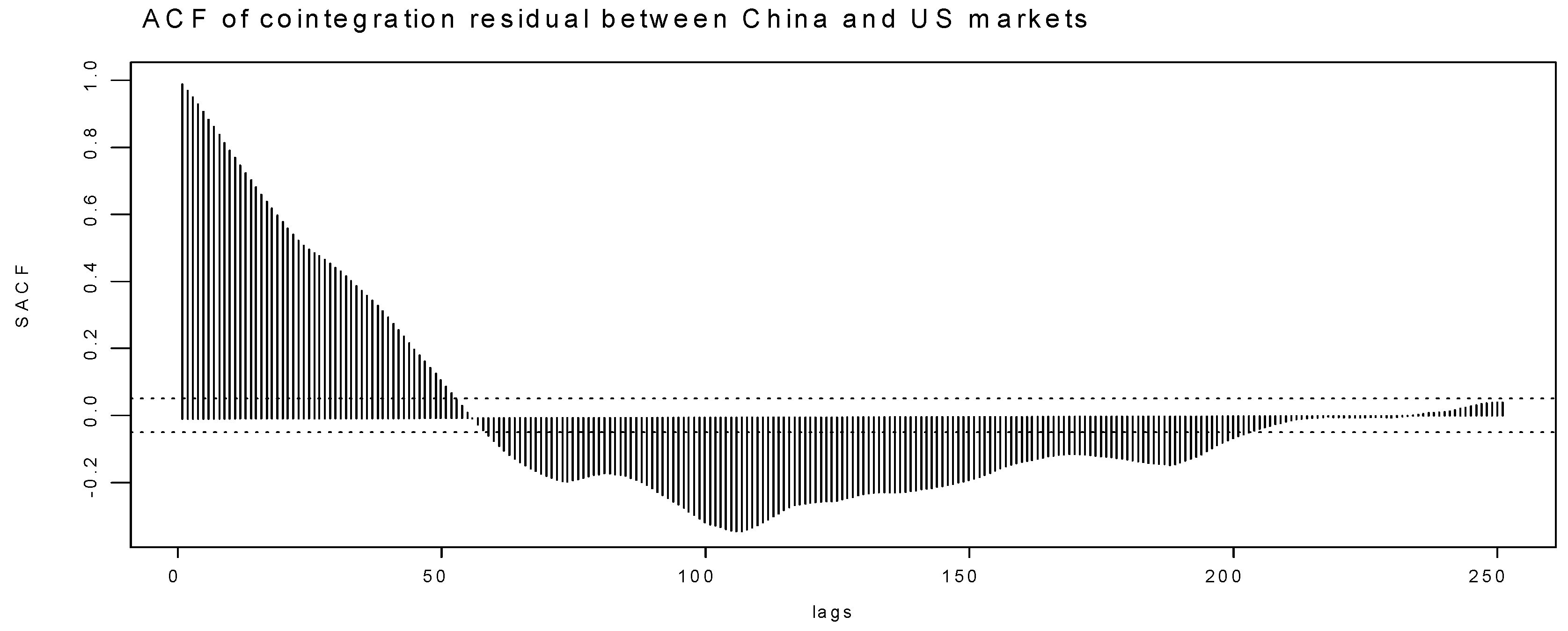

Figure 3.
Sample autocorrelation of cointegration residual series between China and HK
Figure 3.
Sample autocorrelation of cointegration residual series between China and HK
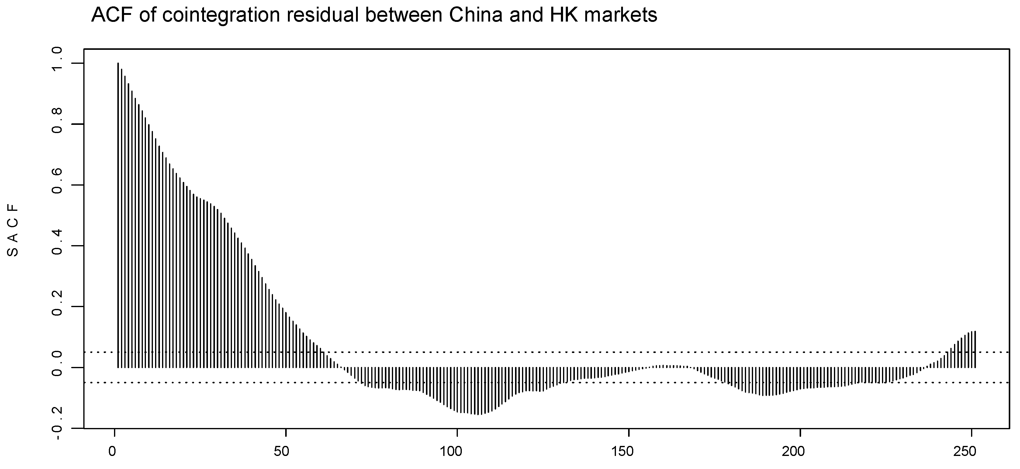
Notes: The two dashed lines denote the 95% confidence interval of the SACF
The pattern of decay for the sample autocorrelation coefficients in both Figure 2 and Figure 3 resembles neither I(1) nor I(0) process for the series being studies in this paper. It decays faster than autocorrelation of I(1) process and exhibits the feature of stationary process, but its autocorrelation has long persistence and cyclic fluctuations. Next, to formally test the possible long range dependence, the R/S test for long memory is applied to these two residual series. The results, which are presented in Table 4, confirm that all the two residual series are fractionally integrated processes presenting long memory property.
Table 4.
Stationarity and long memory tests on cointegration residuals
| Range Over Standard Deviation (R/S) test | |||
| Test statistic | P-value | ||
| 2.7647 | <0.01 | ||
| 3.104 | <0.01 | ||
Notes: , , and are the logs of the weekly Shanghai All Shares index, Hangseng index, and S&P 500 index, respectively. The residual series are constructed by using Equation (2) in the text based on the corresponding DOLS model in Table 3. The bandwidth used in R/S test is integral part of , and N is sample size. The null hypothesis in R/S test is “No long-term dependence.”
Thereafter, we proceed to fit an ARFIMA model as stated in Equation (5) to each of the residual series to estimate the fractional difference parameter in the cointegration residuals. The results are shown in Table 5. From the table, the estimates of d confirm that the two cointegration residual series are fractionally integrated.
Table 5.
ARFIMA fit results
| Value | P-value | Value | P-value | ||
| d | 0.0847 | 0.0170* | 0.0775 | 0.0168* | |
| AR(1) | 0.9665 | 0.0000** | 0.978 | 0.0000** | |
Notes: , , and are the logs of the weekly Shanghai All Shares index, Hangseng index, and S&P 500 index, respectively. The series and are constructed by using equation (2). The superscript stands for dependent variable, while the subscript denotes the independent variable. The choice of AR lags is based on an examination of the ACF and PACF. * , ** significant at the 0.5, 0.01 levels.
To further confirm the results, we test whether the resulting series obtained from applying the ARFIMA model in (5) are I(0) processes9. From the table, the above results confirm that both of two pairs of stock indices, namely and , are fractionally cointegrated.
4.2 Empirical results for China’s and US markets
After the cointegration relations being established in previous section, we proceed to fit the FIVECM model augmented by the MGARCH model. Specifically, we fit the FIVECM-BEKK(1,1) model to the two pairs of differenced index series in logs, i.e. pair of Shanghai All Shares Index and S&P 500; and pair of Shanghai All Shares Index and Hangseng Index; the differenced series are actually the return series of the respective markets. The variable sequences in the fitting FICECM are and in both conditional mean and conditional variance equations, where is dependent variable in both models. An AR(1) structure is employed in FIVECM equations, and multivariate student-t distribution is assumed for the error series of the FIVECM-BEKK (1, 1) models. The fitted model estimates for are exhibited in Table 6.
Table 6.
Estimated coefficients for FIVECM-BEKK(1,1) fitted on
| Parameters | Estimate | Std. Error | t value | Pr(>|t|) |
|---|---|---|---|---|
| C(1) | 0.0006 | 0.0012 | 0.5318 | 0.5950 |
| C(2) | 0.0010 | 0.0009 | 1.1117 | 0.2667 |
| AR(1; 1, 1) | 1.3566 | 0.5104 | 2.6580 | 0.0008*** |
| AR(1; 2, 1) | 0.4766 | 0.3518 | 1.3545 | 0.1761 |
| AR(1; 1, 2) | -1.1648 | 0.5100 | -2.2838 | 0.0227** |
| AR(1; 2, 2) | -0.5968 | 0.3456 | -1.7267 | 0.0848* |
| -1.3188 | 0.5208 | -2.5323 | 0.0011*** | |
| -0.5275 | 0.3530 | -1.4943 | 0.1356 | |
| A(1, 1) | 0.0068 | 0.0018 | 3.7191 | 0.0000*** |
| A(2, 1) | 0.0024 | 0.0014 | 1.7540 | 0.0799* |
| A(2, 2) | 0.0001 | 0.0599 | 0.0011 | 0.9991 |
| ARCH(1; 1, 1) | 0.2496 | 0.0474 | 5.2639 | 0.0000*** |
| ARCH(1; 2, 1) | -0.0043 | 0.0133 | -0.3263 | 0.3721 |
| ARCH(1; 1, 2) | 0.0366 | 0.0671 | 0.5449 | 0.5860 |
| ARCH(1; 2, 2) | 0.2734 | 0.0439 | 6.2276 | 0.0000*** |
| GARCH(1; 1, 1) | 0.9481 | 0.0199 | 47.5456 | 0.0000*** |
| GARCH(1; 2, 1) | 0.0005 | 0.0052 | 0.1034 | 0.4589 |
| GARCH(1; 1, 2) | -0.0025 | 0.0217 | -0.1163 | 0.9074 |
| GARCH(1; 2, 2) | 0.9592 | 0.0138 | 69.190 | 0.0000*** |
Notes: , , and are the logs of the weekly Shanghai All Shares index, Hangseng index, and S&P 500 index, respectively. The estimated model is FIVECM-BEKK(1,1) as shown in (6) and (8), the dependent variable is , the error structure is bivariate t-distribution, and the estimated degrees of freedom are 6.965 with standard error 1.026. The use of the ARFIMA (1,d,0) model reduces the actual sample size to 729. *,**,*** significant at the 10%, 5%, and 1% levels.
In Table 6, the conditional means C(i), i=1,2 are the constant terms in the conditional mean equation, AR(i, j, k), i=1, j=1,2, k=1,2, stand for the AR term coefficients, and , i=1,2, represent the adjustment speed parameters in the FIVECM model displaying in equation (6). The estimates of AR coefficients show that both return series presents serial dependence which is verified by the significant AR(1;2,2) estimates. In particular, the series displays the mean-reversion property as AR(1;2,2) is negative. It is noteworthy to point out that the AR(1; 1,2) is significant, inferring that there is return transmission between stock markets of China and US. In other words, US market Granger-causes China’s market. Conforming to cointegration theory, the sign of the first adjustment speed parameter estimate is correct. The negative value of implies that the Shanghai stock index, , indeed adjusts back to the long-run equilibrium. However, the US stock index, , seems not to be bound by the cointegration relation between the two markets, or the adjustment scheme is only unilateral.
Now, we turn to analyze the conditional variance equation in which A(i, j) denotes the elements of the constant matrix , whereas ARCH(1;i,j) and GARCH(1;i,j) stand for the elements of the ARCH and GARCH coefficient matrices and , respectively. From the table, we observe that all the diagonal elements of coefficient matrices are highly significant, while all the off-diagonal elements are not significant at a conventional significance level. The fitted MARCH model, BEKK(1,1), acts just as the diagonal multivariate volatility model. This result indicates that the GARCH (including ARCH) effects are substantial in the return vector series , which is consistent with usual conclusions about return series. In addition, according to the non-zero values of A(1, 1), the unconditional variances of both return series are not zero, which is confirmed by the Figure 4 for the fitted conditional standard deviation of two return series that show China’s stock market to be much more volatile than the US market.
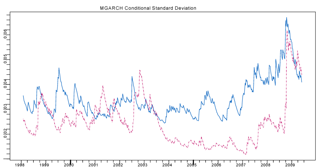
Figure 4.
Conditional Standard Deviations for and
Figure 4.
Conditional Standard Deviations for and

Notes: and are the logs of the weekly Shanghai All Shares index and S&P 500 index, respectively.
The estimated results from the figure indicate no volatility spillover or shock transmission between China and US stock markets. Although there is a long-run conintegrating relationship between the two markets, the information on one market does not immediately influence the other. This could be due to the institutional distinctions, because one is the leading mature market, while the other is a new fledgling one born from the highly-centralized economy. Although the fundamental gaps render the two markets still acting on their own information, the links between the two markets have surely been strengthened by the two increasingly integrated economies. In addition, the elevating contemporaneous relation between China and the US stock markets can be further verified by the evolution of fitted conditional correlation coefficients, as shown in Figure 5.

Figure 5.
Conditional correlation between return series and
Figure 5.
Conditional correlation between return series and
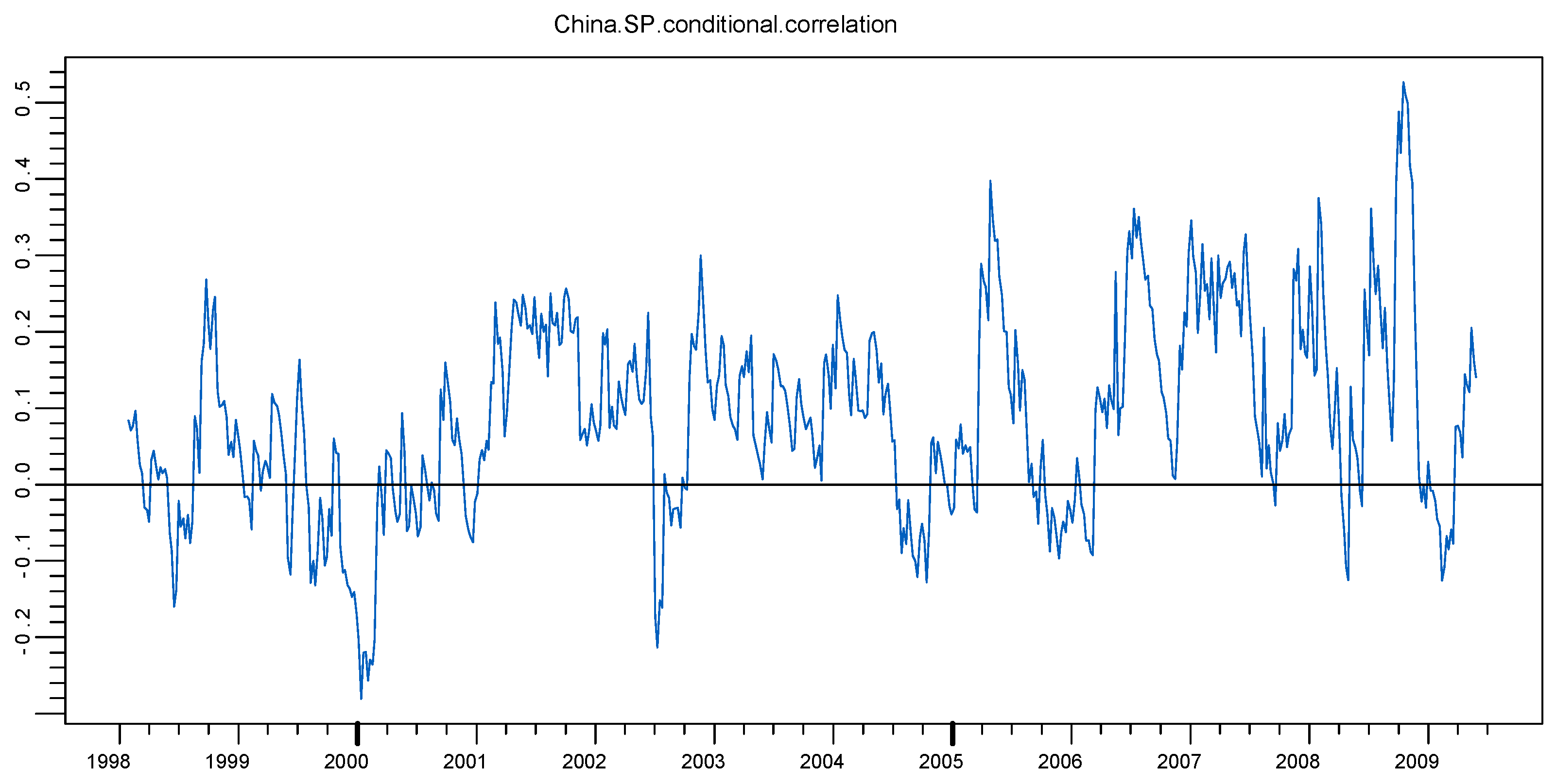
Notes: and are the logs of the weekly Shanghai All Shares index and S&P 500 index, respectively.
Figure 5 shows that there is no obvious long-lasting trend in the conditional correlation over time, howbeit it reveals that the correlation between two market return series has moved upwards a little bit after 2000, interrupted at the late 2002 when there was a collapse on China’s market. At that time, the China’s government attempted to convert huge volume of non-tradable shares (most of them are state-owned shares) to tradable shares10, which could induce panic and crash in the market.
Finally, the eigenvalues of ( and are estimated ARCH and GARCH coefficient matrices, respectively) are 0.997, 0.984, 0.981, and 0.972; all are less than unity. Therefore, the conditional volatilities of two stock return series are stationary. The model adequacy diagnostics are listed in Table 7. Specifically, Ljung-Box test of white noise is applied to both standardized residuals and squared standardized residuals to test for possible remaining serial correlation in the first and second moments of residuals. The number of lags employed in both Ljung-Box tests is 12, indicating that the test statistics follow a Chi-square distribution with 12 degree of freedom. All the tests are applied to the two individual residual series separately. The test statistics show that the fitted model is adequate and successful in capturing the dynamics in the first as well as second moments of index return series.
Table 7.
Model diagnostic statistics for and
| Normality test (Jarque-Bera) | White noise test (Ljung-Box) | GARCH effect test (Ljung-Box) | |||||
| statistic | p-value | statistic | p-value | statistic | p-value | ||
| 22563 | 0.0000* | 9.8954 | 0.1291 | 29.110 | 0.5118 | ||
| 1029 | 0.0000* | 5.0439 | 0.5382 | 26.5266 | 0.6480 | ||
Notes: and are the logs of the weekly Shanghai All Shares index and S&P 500 index, respectively. The Jarque-Bera statistic asymptotically follows a Chi-square distribution with 2 degrees of freedom . The other normality tests like Shapiro-Wilk’s test were also employed, the conclusion is essentially same. These results corroborate the assumption of student-t for the error terms which is based on normality test of original series. * significant at the 1% level.
4.3: Empirical results for China and Hong Kong markets
Table 8 exhibits the coefficient estimates for the FIVECM-BEKK(1,1) fitted on the other pair of return series, i.e. , representing China and Hong Kong markets.
Table 8.
Estimated coefficients for FIVECM-BEKK(1,1) fitted on
| Parameters | Value | Std. Error | t value | Pr(>|t|) |
|---|---|---|---|---|
| C(1) | 0.0006 | 0.0001 | 0.5295 | 0.5966 |
| C(2) | 0.0018 | 0.0013 | 1.3873 | 0.1659 |
| AR(1; 1, 1) | 0.9468 | 0.2593 | 3.6506 | 0.000*** |
| AR(1; 2, 1) | -0.0352 | 0.2581 | -0.1367 | 0.8913 |
| AR(1; 1, 2) | -0.8387 | 0.2683 | -3.1255 | 0.0018*** |
| AR(1; 2, 2) | -0.0095 | 0.2637 | -0.0359 | 0.9713 |
| -0.9248 | 0.2674 | -3.4582 | 0.0000*** | |
| -0.0331 | 0.2617 | -0.1263 | 0.8995 | |
| A(1, 1) | 0.0077 | 0.0018 | 4.0790 | 0.0000*** |
| A(2, 1) | 0.0019 | 0.0021 | 0.8992 | 0.3689 |
| A(2, 2) | 0.0000 | 0.1503 | 0.0003 | 0.9997 |
| ARCH(1; 1, 1) | 0.2683 | 0.0510 | 5.2569 | 0.0000*** |
| ARCH(1; 2, 1) | 0.1033 | 0.0523 | 1.9729 | 0.0489** |
| ARCH(1; 1, 2) | -0.0296 | 0.0438 | -0.6754 | 0.4997 |
| ARCH(1; 2, 2) | 0.2192 | 0.0549 | 3.9899 | 0.0000*** |
| GARCH(1; 1, 1) | 0.9318 | 0.0257 | 36.1752 | 0.0000*** |
| GARCH(1; 2, 1) | 0.0138 | 0.0069 | 2.0222 | 0.0217** |
| GARCH(1; 1, 2) | 0.0137 | 0.0127 | 1.0748 | 0.2829 |
| GARCH(1; 2, 2) | 0.9773 | 0.0148 | 65.709 | 0.0000*** |
Notes: and are the logs of the weekly Shanghai All Shares index and Hangseng index, respectively. The estimated model is FIVECM-BEKK(1,1) as stated in (6) and (8): the dependent variable is , the error structure is bivariate t-distribution, and the estimated degrees of freedom are 7.029 with standard error 1.142. The use of an ARFIMA (1,d,0) model reduces the actual sample size to 729. *, *, ** significant at the 10%, 5%, and 1% levels.
Overall, the results in Table 8 show a stronger relationship between China and Hong Kong markets than that between China and US markets, this is unsurprising because the two economies are closely related and interdependent on each other. For the AR terms, the significance of AR(1; 1, 1) indicates there is serial correlation in China’s stock market while the opposite is true for Hong Kong’s stock market because AR(1; 2,2) is insignificant. The significant AR(1;1,2) signifies that there is return transmission from Hong Kong to China’s market. This could be due to the exemplary role of Hong Kong to China’s Stock market, as Hong Kong has historically been a good reference for China in establishing and toning its stock market. Next, the highly significant with right sign dictates that China’s stock index is also restricted by the long-run equilibrium with Hong Kong market. Again, the adjustment to the cointegration relation is unilateral, as Hong Kong market appears not to respond to disequilibrium between the two markets.
Finally, the estimates for the conditional variances show an interesting interaction between the volatility processes of the two markets. In particular, the significance of both GARCH(1; 2, 1) and ARCH(1; 2, 1) suggests that the volatility spillover goes from China’s market to Hong Kong’s market. Furthermore, the information transmission is unidirectional because the other two off-diagonal coefficients are not statistically different from zero. The information flow may reflect the fact that the economy of Hong Kong heavily relies on mainland China, and a substantial part of foreign direct investment (FDI) in mainland China is from Hong Kong. Thus, information about macroeconomic conditions and policies as well as micro-market structures in the mainland would certainly exert a great deal of repercussions on the Hong Kong stock market. In addition, many large state-owned inland companies listed in the Hong Kong exchange (some of them are cross-listed in both markets) may also contribute to passing market shocks from mainland China to Hong Kong. In this sense, China’s stock marking leads in comparison to the Hong Kong market in information absorption. Also, the significant diagonal elements of ARCH and GARCH matrices confirm the property of conditional heteroskedasticity of two return series. The fitted conditional standard deviations of two series are shown in Figure 6 which also affirms the higher variability of mainland China’s market than Hong Kong market.

Figure 6.
Conditional Standard Deviations for and
Figure 6.
Conditional Standard Deviations for and
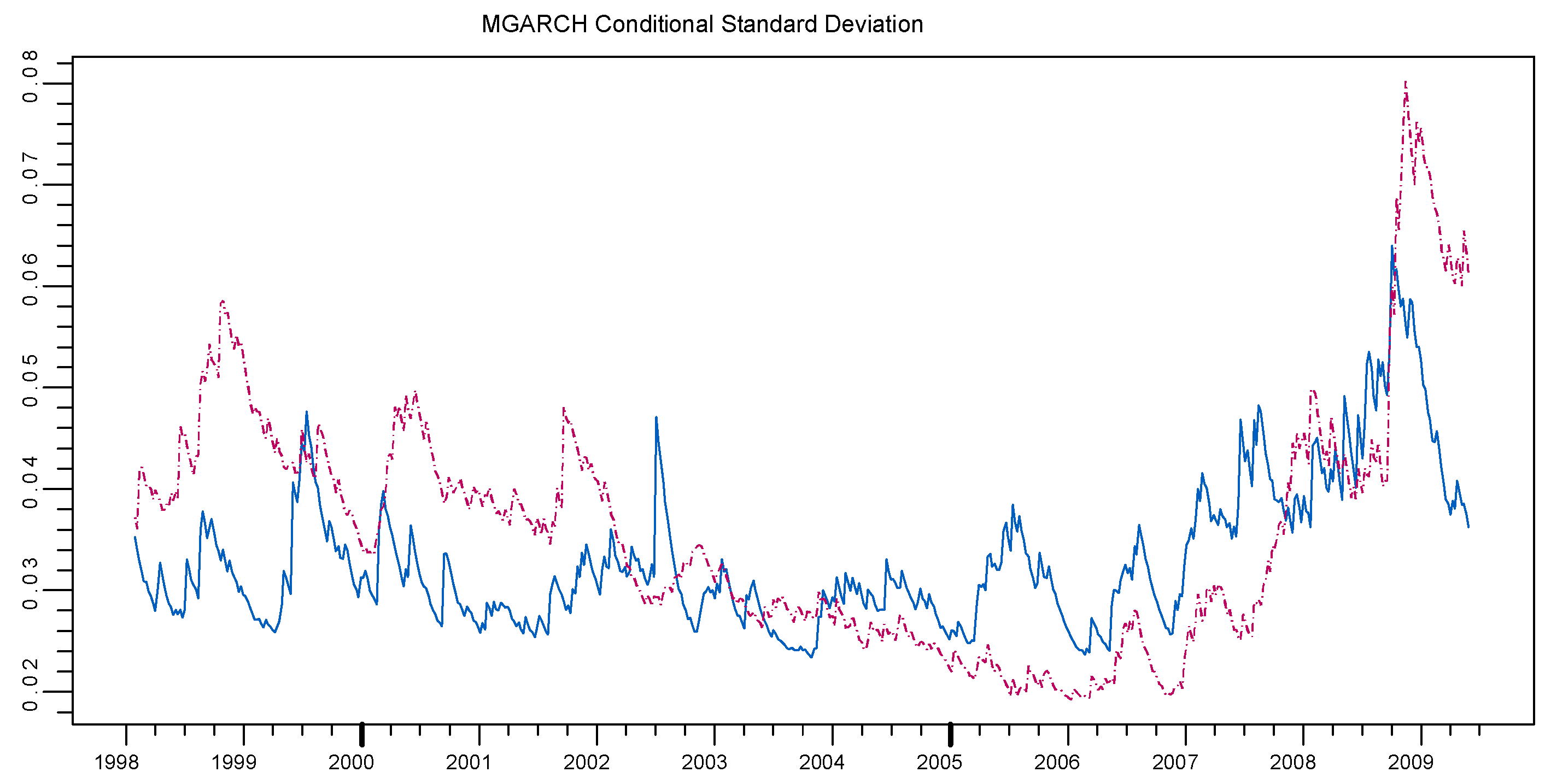
Notes: and are the logs of the weekly Shanghai All Shares index and Hangseng index, respectively.
In addition, Figure 7 below describes the dynamics of contemporaneous correlation between the two index return series, and . The fitted conditional correlation between the two return series was quite volatile before mid-2001, whereas afterwards it is less volatile and gradually stabilizes in the positive range with few interruptions, a typical example of this is in late 2002 when China’s stock market collapsed. This pattern coincides with the increasing institutional and economic links between the two sides after the sovereignty of Hong Kong was returned to China.
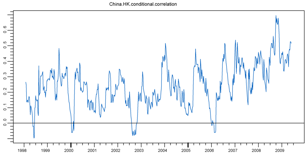
Figure 7.
Conditional correlation between return series and
Figure 7.
Conditional correlation between return series and

Notes: and are the logs of the weekly Shanghai All Shares index and Hangseng index, respectively.
Comparing Figure 7 with Figure 5, it is obvious that the positive range of conditional correlation between China and Hong Kong markets is larger than that between China and the US markets. Indeed, the median of the former contemporaneous correlation is 0.087, whereas that of the latter is -0.032. The model diagnostic below shows the adequacy of the FIVECM-BEKK(1,1) model fitted on and .
Table 9.
Model diagnostic statistics for and
| Normality test (Jarque-Bera) | White noise test (Ljung-Box) | GARCH effect test (Ljung-Box) | |||||
| statistic | p-value | statistic | p-value | statistic | p-value | ||
| 1098 | 0.0000 | 44.278 | 0.0450 | 30.214 | 0.4547 | ||
| 49.73 | 0.0000 | 30.460 | 0.4422 | 22.4701 | 0.8364 | ||
Notes: and are the logs of the weekly Shanghai All Shares index and Hangseng index, respectively. The Jarque-Bera statistic asymptotically follows Chi-square distribution with 2 degrees of freedom. The other normality tests like Shapiro-Wilk’s test has also been employed, the conclusion is essentially same. These results corroborate the assumption of student-t for the error terms which is based on normality test of original series.
Again, as the eigenvalues of are 0.996, 0.977, 0.977, and 0.970; all are less than unity, the fitted conditional volatilities of China and Hong Kong stock return series are again confirmed to be stationary.
5. CONCLUSION
This paper employed the FIVECM model to investigate the cointegration relations between China and the US stock markets, and between China and Hong Kong stock markets. Applying the Engle-Granger two-step procedure to estimate and construct the cointegration vector, this paper set up the FIVECM in the general VAR framework which can be used to reveal the long-run equilibrium, short-run dynamic movement, as well as lead-lag relations between the index return series. Furthermore, by augmenting the FIVECM model by MGARCH model, the dynamic dependences in the second conditional moments of index return series are also brought into the picture.
The empirical results confirm our conjecture that there are fractional cointegration relations, or long-run equilibria between China and the US stock markets, and between China and Hong Kong stock markets. However, according to the estimates, only China’s market appears to be bound by the cointegration relations; the other two markets do not make adjustments in response to the deviations from the equilibrium. The US and Hong Kong markets are also found to lead China’s market in first conditional moments; that is, there are return transmissions running from both US and Hong Kong markets to China’s market. This finding is expected, as both the US and Hong Kong are more developed and mature markets, China’s stock market investors are likely to follow precedent and trail after what their counterparts have done previously in the US and Hong Kong. However, volatility spillover effect is shown by estimates to flow from China’s market into Hong Kong’s market; in other words, there is information transmission from mainland China into the Hong Kong market. This may well be due to the heavy dependence of the economy of Hong Kong on the mainland, and the increasing number of cross-listed companies on both markets.
The evolution of the two fitted conditional correlation series reveal that China’s stock market has been experiencing stronger and more stable ties with both the US and Hong Kong markets in recent years. Moreover, judging from the magnitude of dynamic correlation coefficients, China’s market appears to be closer to Hong Kong’s market than the US market, specifically- China’s stock market is more positively correlated with its close neighboring market than with the world’s leading superpower. This finding provides important information to international portfolio managers investing on these three markets.
Overall speaking, although China’s stock market has a long-run cointegration relation with the world market, represented by the US and Hong Kong markets, the short-run interactions, namely return and volatility transmissions, between China’s market and the other markets are not profuse. We believe that the ongoing liberalization and deregulation in China’s financial market may increase the integration of its stock market further into world markets. In terms of future research, this paper only exploits the stock market indices and their differenced series; incorporating other relevant exogenous variables into the model may shed some additional light on the results.
ACKNOWLEDGMENTS
This paper is funded by a research grant at Southwestern University of Finance and Economics ( 211 Project, Phase III ).
References
- R.T Baillie. “Long memory processes and fractional integration in econometrics.” Journal of Econometrics 73 (1996): 5–59. [Google Scholar]
- R.T. Baillie, and et al. “Analyzing Inflation by the Fractionally Integrated Arfima-GARCH model.” Journal of Applied Econometrics Vol.11, No.1 (1996): 23–40. [Google Scholar]
- R.T. Baillie, and T. Bollerslev. “Cointegration, fractional cointegration and exchange rate dynamics.” The Journal of Finance Vol. 49, No. 2 (1994): 737–745. [Google Scholar]
- L Bauwens, S. Laurent, and J. Rombouts. “Multivariate GARCH models: a survey.” Journal of Applied Econometrics 21, 1 (2006): 79–109. [Google Scholar]
- H. Chen, R. Smyth, and W.K. Wong. “Is Being a Super-Power More Important Than Being Your Close Neighbor? Effects of Movements in the New Zealand and United States Stock Markets on Movements in the Australian Stock Market.” Applied Financial Economics 18, 9 (2008): 1–15. [Google Scholar]
- Y. Cheung, and K. Lai. “A fractional cointegration analysis of purchasing power parity.” Journal of Business and Economic Statistics 11 (1993): 103–112. [Google Scholar]
- Y.L. Cheung, and S.C. Mak. “The international transmission of stock market fluctuation between the developed markets and the Asian-Pacific markets.” Applied Financial Economics 2 (1992): 43–47. [Google Scholar]
- Y.W Cheung, and L.K. Ng. “Stock price dynamics and firm size: an empirical investigation.” Journal of Finance 47 (1992): 1985–1997. [Google Scholar]
- W. Chou, and Y. Shih. “Long-run purchasing power parity and long-term memory: evidence from Asian newly industrialized countries.” Applied Economics Letters 4 (1997): 575–578. [Google Scholar]
- P.J. Chung, and D.J. Liu. “Common stochastic trends in Pacific Rim stock markets.” Quarterly Review of Economics and Finance 34 (1994): 241–259. [Google Scholar]
- A. Corhay, A. Rad, and J. Urbain. “Long-run behavior of Pacific-Basin stock prices.” Applied Financial Economics 5 (1995): 11–18. [Google Scholar]
- K.J. Daly. “Southeast Asian stock market linkages : evidence from pre-and post-October 1997.” ASEAN Economic Bulletin 20 (2003): 73–85. [Google Scholar]
- D.A. Dickey, and W.A. Fuller. “Distribution of the estimators for autoregressive time series with a unit root.” Journal of the American Statistical Association 74 (1979): 427–431. [Google Scholar]
- D.A. Dickey, and W.A. Fuller. “Likelihood ratio statistics for autoregressive time series with a unit root.” Econometrica 49 (1981): 1057–1072. [Google Scholar]
- G. Dwyer, and M. Wallace. “Cointegration and market efficiency.” Journal of International Money and Finance 11 (1992): 318–327. [Google Scholar]
- R. Engle, and C.W.J. Granger. “Cointegration and error correction: representation, estimation and testing.” Econometrica 55 (1987): 251–276. [Google Scholar]
- R.F. Engle, and F.K. Kroner. “Multivariate simultaneous generalized ARCH.” Econometric Theory 11 (1995): 122–150. [Google Scholar]
- C.S. Eun, and S. Shim. “International transmission of stock market movements.” Journal of Financial and Quantitative Analysis 24 (1989): 41–56. [Google Scholar]
- J.L. Fernandez-Serrano, and S. Sosvilla-Rivero. “Modelling evolving long-run relationships: the linkages between stock markets in Asia.” Japan and the World Economy 13 (2001): 145–160. [Google Scholar]
- J.L. Fernandez-Serrano, and S. Sosvilla-Rivero. “Modelling the linkages between US and Latin American stock markets.” Applied Economics 35 (2003): 1423–1434. [Google Scholar]
- W.M. Fong, W.K. Wong, and H.H. Lean. “Stochastic dominance and the rationality of the momentum effect across markets.” Journal of Financial Markets 8 (2005): 89–109. [Google Scholar]
- J. Geweke, and S. Porter-Hudak. “The estimation and application of long memory time series models.” Journal of Time Series Analysis 4 (1983): 221–238. [Google Scholar]
- C.W.J. Granger. “Long memory relationships and the aggregation of dynamic models.” Journal of Econometrics 14 (1981): 227–238. [Google Scholar]
- C. W. J. Granger. “Developments in the study of cointegrated economic variables.” Oxford Bulletin of Economics and Statistics 48 (1986): 213–228. [Google Scholar]
- C.W.J. Granger. “Some recent developments in a concept of causality.” Journal of Econometrics 39 (1988): 213–228. [Google Scholar]
- C.W.J. Granger, B.N. Huang, and C.W. Yang. “A bivariate causality between stock prices and exchange rates: evidence from recent Asian flu.” Quarterly Review of Economics and Finance 40 (2000): 337–354. [Google Scholar]
- A.W. Gregory, and B.E. Hansen. “Residual-based tests for cointegration in models with regime shifts.” Journal of Econometrics 70 (1996): 99–126. [Google Scholar]
- H.G. Grubel. “Internationally diversified portfolios: welfare gains and capital flows.” American Economic Review 58 (1968): 1299–1314. [Google Scholar]
- J. Haslett, and A. E. Raftery. “Space-time Modeling with Long-Memory Dependence: Assessing Ireland’s Wind Power Resource.” Journal of Royal Statistical Society Series C 38 (1989): 1–21. [Google Scholar]
- C. Hsiao. “Autoregressive modeling of Canadian money and income data.” Journal of the American Statistical Association 74 (1979): 553–560. [Google Scholar]
- C. Hsiao. “Autoregressive modelling of money income causality detection.” Journal of Monetary Economics 7 (1981): 85–106. [Google Scholar]
- B.N. Huang, C.W. Yang, and J.W.S. Hu. “Causality and cointegration of stock markets among the United States, Japan and the South China Growth Triangle.” International Review of Financial Analysis 9 (2000): 281–297. [Google Scholar]
- H.E. Hurst. “Long-term storage capacity of reservoirs.” Transactions of the American Society of Civil Engineers 116 (1951): 770–799. [Google Scholar]
- S. Johansen. “The mathematical structure of error correction models.” Contemporary Mathemetics 8 (1988a): 359–386. [Google Scholar]
- S. Johansen. “Statistical analysis of cointegration vector.” Journal of Economic Dynamics and Control 12 (1988b): 231–254. [Google Scholar]
- S. Johansen. Likelihood-inference in cointegrated vector autoregressive models. Oxford: Oxford University Press, 1995. [Google Scholar]
- R. Johnson, and L. Soenen. “Asian economic integration and stock market comovement.” Journal of Financial Research 25 (2002): 141–157. [Google Scholar]
- K. Kasa. “Common stochastic trends in international stock markets.” Journal of Monetary Economics 29 (1992): 95–124. [Google Scholar]
- G. Koop. “An objective Bayesian analysis of common stochastic trends in international stock prices and exchange rates.” Journal of Empirical Finance 1 (1994): 343–364. [Google Scholar]
- S.B. Lee, and K.J. Kim. “Does the October 1987 crash strengthen the co-movement in stock price indexes.” Quarterly Review of Economics and Business 3 (1994): 89–102. [Google Scholar]
- D.R. Lessard. “World, national and industry factors in equity returns.” Journal of Finance 29 (1974): 379–391. [Google Scholar]
- H. Levy, and M. Sarnat. “International diversification of investment portfolios.” American Economic Review 60 (1970): 668–675. [Google Scholar]
- D. Lien, and Y. Tse. “Fractional Cointegration and Futures Hedging.” The Journal of Futures Markets 19 (1999): 457–474. [Google Scholar]
- A.W. Lo, and A.C. MacKinlay. “Stock market prices do not follow random walks: Evidence from a simple specification test.” Review of Financial Studies 1 (1988): 41–66. [Google Scholar]
- A.M.M. Masih, and R. Masih. “Dynamic linkages and the propagation mechanism driving major international stock markets: an analysis of the pre-and-post-crash eras.” Quarterly Review of Economics and Finance 37 (1997): 859–888. [Google Scholar]
- A.M.M. Masih, and R. Masih. “Are Asian stock market fluctuations due mainly to intra-regional contagion effects? Evidence based on Asian emerging stock markets.” Pacific Basin Finance Journal 7 (1999): 251–282. [Google Scholar]
- A.M.M. Masih, and R. Masih. “Propagative causal price transmission among international stock markets: evidence from the pre-and-post globalization period.” Global Finance Journal 13 (2002): 63–91. [Google Scholar]
- P.K. Narayan, and R. Smyth. “Are OECD stock prices characterized by a random walk? evidence from sequential trend break and panel data models.” Applied Financial Economics 15 (2005): 547–556. [Google Scholar]
- T.H. Ng. “Stock market linkages in Southeast Asia.” Asian Economic Journal 16 (2002): 353–377. [Google Scholar]
- S. Ng, and P. Perron. “Unit Root Tests in ARMA Models with Data-Dependent Methods for the Selection of the Truncation Lag.” Journal of the American Statistical Association 90 (1995): 268–281. [Google Scholar]
- M.S. Pan, Y.A. Liu, and H.J. Roth. “Common stochastic trends and volatility in Asian-Pacific equity markets.” Global Finance Journal 10 (1999): 161–172. [Google Scholar]
- P.C.B. Phillips, and P. Perron. “Testing for a unit root in time series regression.” Biometrika 75 (1988): 335–346. [Google Scholar]
- D.M. Ripley. “Systematic elements in the linkage of national stock market indices.” Review of Economics and Statistics 55 (1973): 356–361. [Google Scholar]
- K. Shimotsu, and P.C.B. Phillips. “Exact Local Whittle Estimation of Fractional Integration.” The Annals of Statistics 33, 4 (2005): 1890–1933. [Google Scholar]
- P.L. Siklos, and P. Ng. “Integration among Asia-Pacific and international stock markets: common stochastic trends and regime shifts.” Pacific Economic Review 6 (2001): 89–110. [Google Scholar]
- C. Sims, and J.H. Stock. “Inference in linear time series models with some unit roots.” Econometrica 58 (1990): 113–144. [Google Scholar]
- J.H. Stock, and M.W. Watson. “A simple estimator of cointegrating vectors in higher order integrated systems.” Econometrica 61 (1993): 783–820. [Google Scholar]
- G.M. Von Furstenberg, and B.N. Jeon. “International stock price movements: links and messages.” Brookings Papers on Economic Activity, 1989, 125–179. [Google Scholar]
- 1Except mild restrictions imposed on the elements of coefficients matrices in order to ensure identification of BEKK(1,1) model. Readers may refer to Propositions 2.1-2.3 of Engle and Kroner (1995) for more information.
- 2Shanghai All Shares index is the most commonly quoted index to represent China’s stock market, because most large (especially state-owned) companies are listed in Shanghai stock exchange (SHSE). The market capitalization of Shenzhen Stock Exchange is about half that of SHSE, and thus, it is less used to represent China’s stock market.
- 3This means that the estimate converges to true value at faster rate than usual OLS estimate.
- 4This is actually one particular cointegration called C(1,1) as termed in Granger (1986). The general concept of cointegration is that if I (d) random vector has a linear combination which is I(b) process, , then the component series of are said to be cointegrated, denoted as C(d,b).
- 5The Approximate MLE is based on the procedure of Haslett & Raftery (1989) which essentially approximates infinite autoregressive coefficients in ARFIMA model by asymptotic values. The log-likelihood function for estimation is actually the concentrated one.
- 6The complete form of BEKK in Engle and Kroner (1995) accommodates more generality, interested readers are referred to the original paper; the model (7) here is essentially BEKK(1,p,q) in their paper.
- 7 Readers may refer to Proposition 2.7 of Engle and Kroner (1995) for detailed discussion on covariance stationarity conditions for the general BEKK model.
- 8We then test the null hypothesis H0: I(2) versus the alternative hypothesis that H1: I(1) but the results reject I(2).
- 9The ADF and PP tests confirm the results.
- 10Non-tradable shares, which are of the form of state shares and legal entity shares alike, account for about two thirds of the total shares issued on China’s domestic exchanges.