The Nexus between Analyst Forecast Dispersion and Expected Returns Surrounding Stock Market Crashes


Abstract
:1. INTRODUCTION
2. DATA AND METHODOLOGY
- Criterion 1
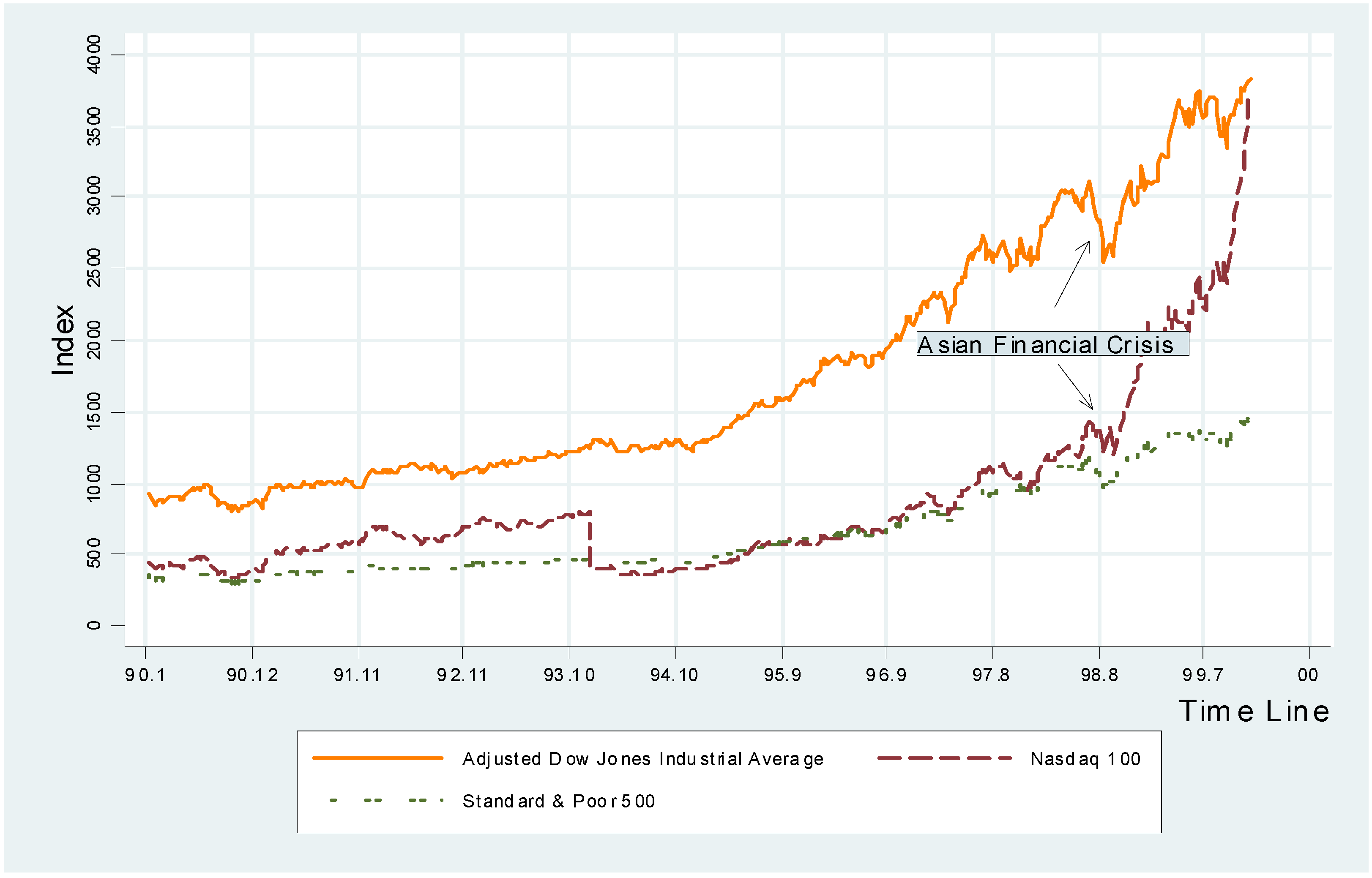
- All the three indices must fall by more than 30% during the crashes.
- Criterion 2
- a. At the beginning of a crash, at least two of the indices reach a two-year high, and at least two of them fall by more than 15% in the following two months.b. At the end of a crash, at least two of the indices reach a two-year low, and at least two of them rise by more than 15% in the following two months.
3. ANALYST FORECAST DISPERSION (AFD)
4. FAMA-FRENCH THREE-FACTOR MODEL
5. CONCLUSION

| Available since | Covered companies | Characters of companies | Covered Countries | Methodology | |
|---|---|---|---|---|---|
| DJIA | 1896 | 30 | Largest and most widely held public companies. | U.S. | Price-weighted, scaled if there were stock splits. |
| Nas100 | January 1985 | 100 | Largest domestic and international non-financial companies. | All | Modified value-weighted. |
| SP500 | 1957 | 500 | Large publicly held companies. | Mostly U.S. | Market value-weighted. |
| DJ | Nasdaq | SP500 | ||||
|---|---|---|---|---|---|---|
| Starting | Ending | Starting | Ending | Starting | Ending | |
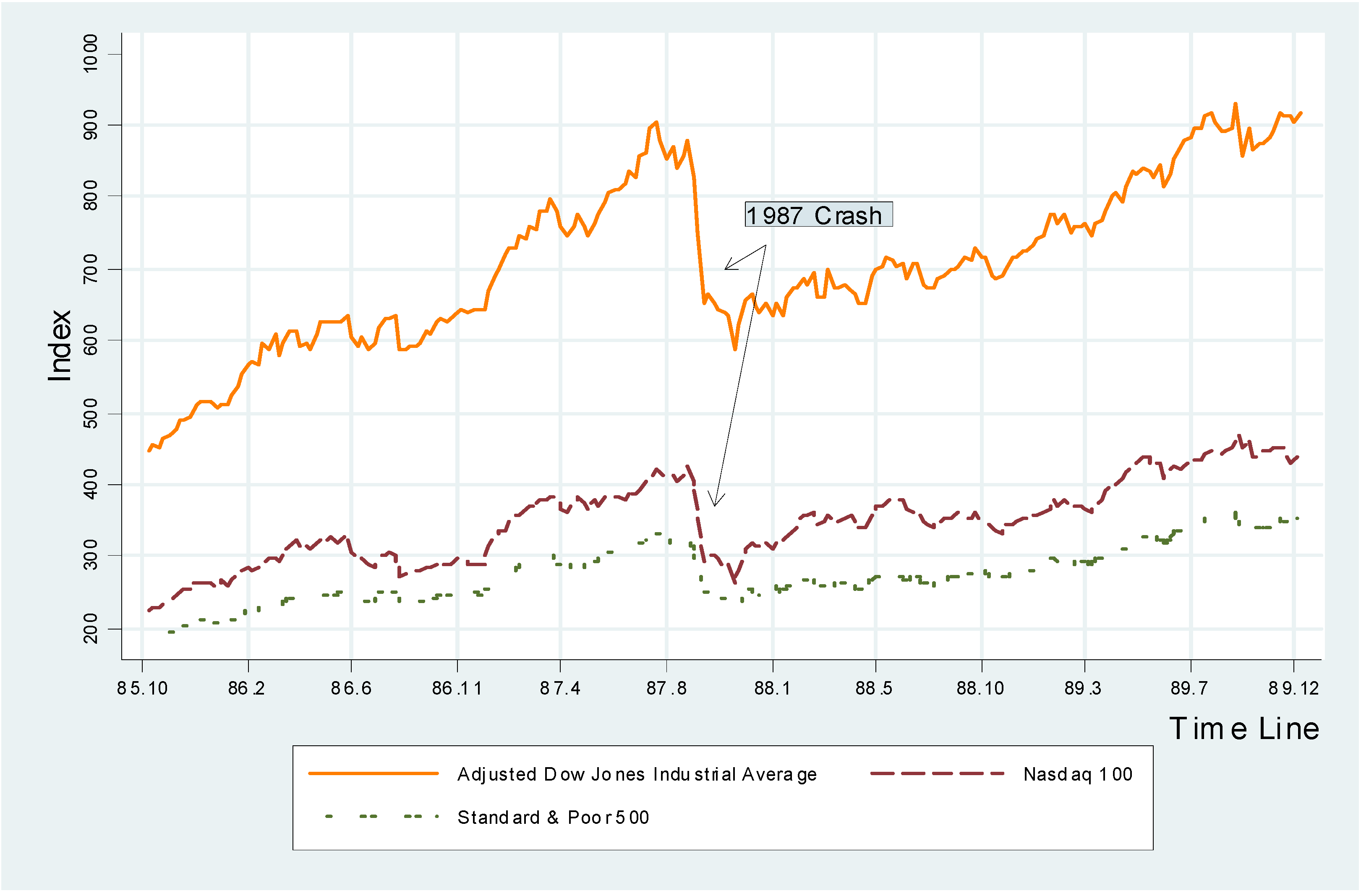
| 1987 crash | 1987.8.17 | 1987.11.30 | 1987.8.17 | 1987.11.30 | 1987.8.17 | 1987.11.30 |
| Index | 2709.5 | 1766.74 | 421.15 | 260.87 | 335.9 | 223.92 |
| Peak/Trough | Yes | Yes | No | Yes | Yes | Yes |
| % Fall(-)/Rise in 2 months | -28.00 | 10.84 | -30.95 | 22.00 | -26.11 | 15.80 |
| Duration | 3.5 month | 3.5months | 3.5 months | |||
| % Index change in total | -34.79 | -38.06 | -33.33 | |||
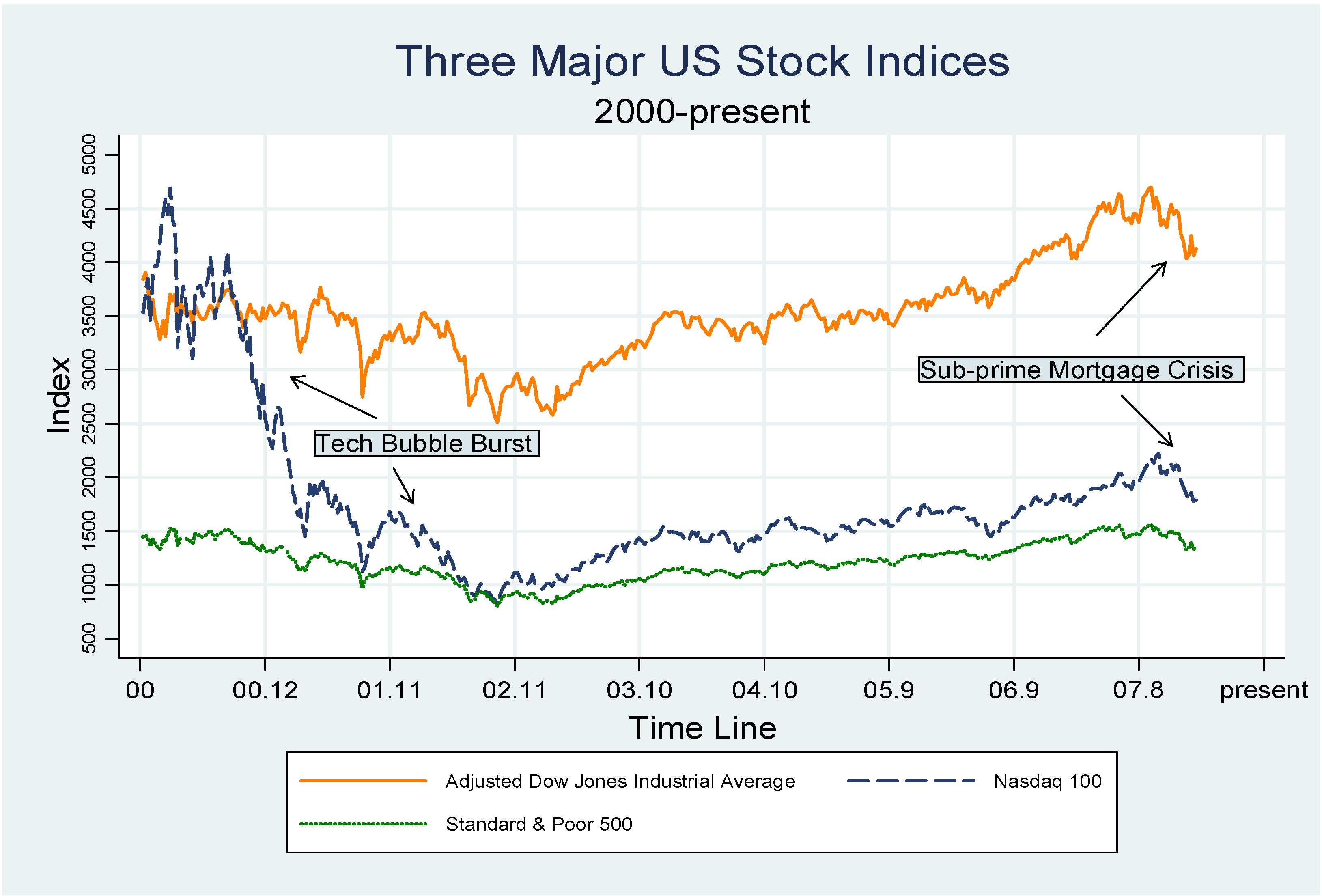
| 00-02 tech-bubble burst | 2000.3.20 | 2002.9.30 | 2000.3.20 | 2002.9.30 | 2000.3.20 | 2002.9.30 |
| Index | 11112.72 | 7528.4 | 4691.61 | 815.4 | 1527.46 | 800.58 |
| Peak/Trough | No | Yes | Yes | Yes | Yes | Yes |
| % Fall(-)/Rise in 2 months | -7.32 | 18.17 | -33.89 | 36.93 | -19.70 | 17.00 |
| Duration | 2.5 years | 2.5 years | 2.5 years | |||
| % Index change in total | -32.25 | -82.62 | -47.59 | |||
| Factor Sensitivities | ||||||
|---|---|---|---|---|---|---|
| Rm – Rf | SMB | HML | Adj. R2 | |||
| D1(low dispersion) | 1 | 0.722 | 0.253 | 0.084 | 0.73 | |
| Newey Adj. t | (3.50) ** | (12.48) ** | (3.71) ** | (4.32) ** | ||
| D2 | 0.6 | 0.823 | 0.395 | 0.046 | 0.8 | |
| Newey Adj. t | (2.60) * | (13.12) ** | (7.39) ** | (2.50) * | ||
| D3 | 0.3 | 1.016 | 0.537 | -0.032 | 0.85 | |
| Newey Adj. t | -0.97 | (12.14) ** | (10.55) ** | (-1.09) | ||
| D4 | -0.1 | 1.182 | 0.652 | -0.144 | 0.87 | |
| Newey Adj. t | (-0.39) | (14.20) ** | (9.20) ** | (-2.83) ** | ||
| D5(high dispersion) | 0.07 | 1.455 | 0.833 | -0.224 | 0.9 | |
| Newey Adj. t | -0.16 | (15.92) ** | (8.14) ** | (-2.86) ** | ||
| Tests for ARCH effect and Serial Correlations | ||||||
| ARCH effect | Serial correlation | |||||
| P-value | P-value | P-value | conclusion | DW statistic | conclusion | |
| Regression | (lag1) | (lag2) | (lag3) | |||
| D1 | 0.94 | 0.31 | 0.36 | No ARCH | 1.57 | Uncertain |
| D2 | 0.94 | 0.62 | 0.7 | No ARCH | 1.56 | Uncertain |
| D3 | 0.6 | 0.91 | 1.21 | No ARCH | 1.77 | No SC |
| D4 | 0.49 | 0.54 | 0.14 | No ARCH | 1.92 | No SC |
| D5 | 0.31 | 0.47 | 0.44 | No ARCH | 1.91 | No SC |
| Factor Sensitivities | |||||||
|---|---|---|---|---|---|---|---|
| Dep. Variable: excess returns | Alpha(%) | Rm - Rf | SMB | HML | Dispersion | Dispersion2 | Adj. R2 |
| Loadings | -0.32 | 1.04 | 0.53 | -0.05 | 0.04 | 0.89 | |
| Newey Adj. t | (-0.22) | (16.90) ** | (10.80) ** | (-1.51) | (0.49) | ||
| Loadings | 10.80 | 1.04 | 0.54 | -0.06 | -1.45 | 4.77 | 0.90 |
| Newey Adj. t | (2.01) * | (17.43) ** | (10.08) ** | (-2.77) ** | (-2.09) * | (2.20) * | |


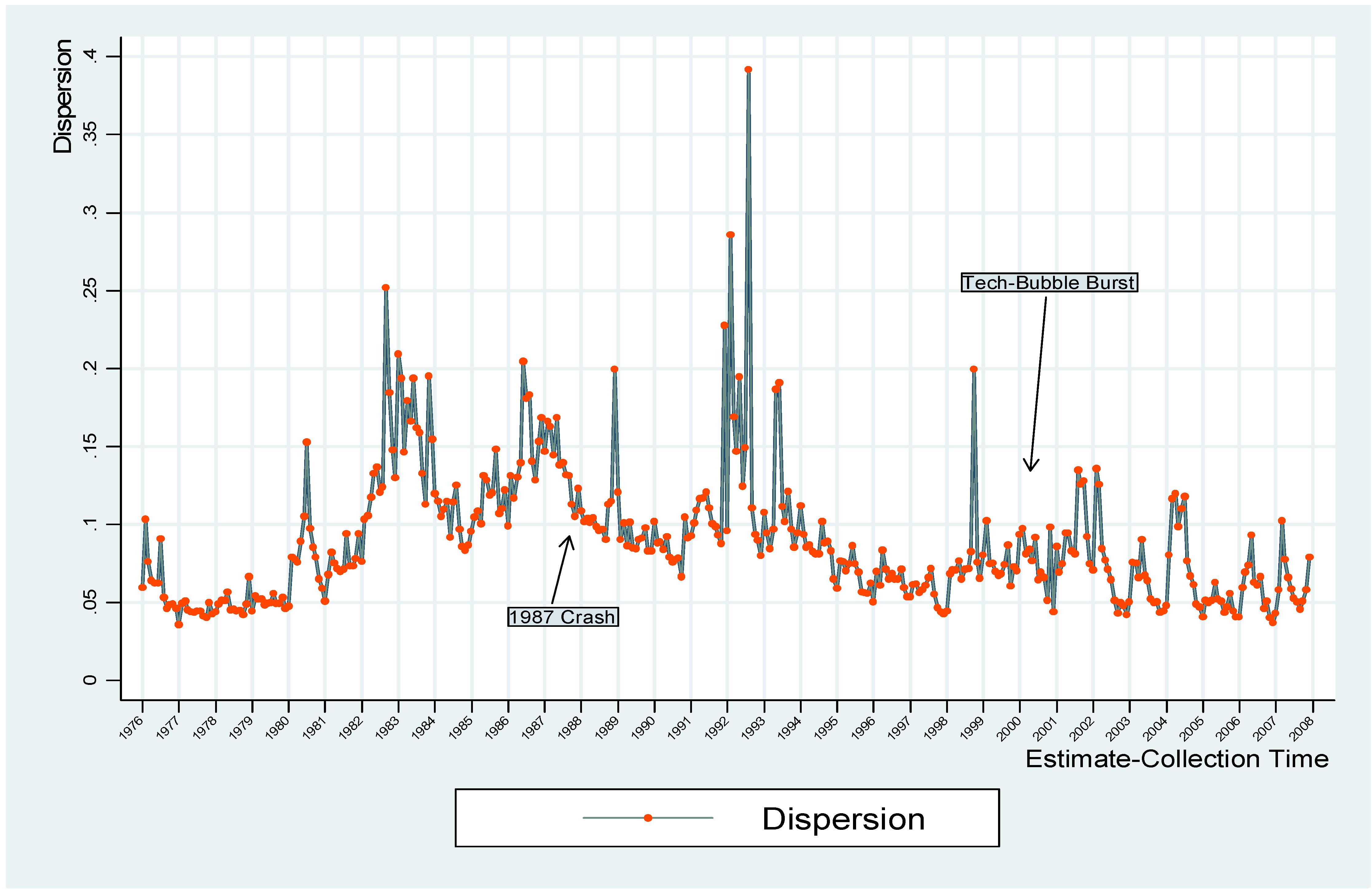
- 1The estimates contained in the Summary File are collected and filtered from the Detail History File on the third Thursday of each month.
- 3Bry and Boschan (1971) use a nonparametric approach to partition a time series into two half cycles. Pagan and Sossounov (2003) adopt the Bry-Boschan (BB) algorithm to define the bull-bear cycles of the market. Chong et al. (2010) use the moving-average crossing rule to define market states.
- 4The 1987 sub-sample contains only 29 monthly observations, which is inadequate for us to conduct a meaningful regression analysis.
- 5We use the Goldilocks method to determine the lag length, i.e. m = 0.75T1/3, where m is the lag length, T is the sample size. A lag length of 3 is used as a result. The method is discussed in Newey and West (1987).
ACKNOWLEDGMENTS
REFERENCE
- B.B. Ajinkya, and M.J. Gift. “Dispersion of financial analysts' earnings forecasts and the (option model) implied standard deviations of stock returns.” Journal of Finance 40, 5 (1985): 1353–1365. [Google Scholar]
- G. Bry, and C. Boschan. “Cyclical analysis of time series: Selected procedures and computer programs.” New York: NBER, 1971. [Google Scholar]
- R.M. Bushman, J.D. Piotroski, and Abbie J. Smith. “Insider trading restrictions and analysts’ incentives to follow firms.” Journal of Finance 60, 1 (2005): 35–66. [Google Scholar]
- X. Chang, Sudipto Dasgupta, and Gilles Hilary. “Analyst coverage and financing decisions.” Journal of Finance 61, 6 (2006): 3009–3048. [Google Scholar]
- J. Chen, H. Hong, and J.C. Stein. “Breadth of ownership and stock returns.” Journal of Financial Economics 66, 2-3 (2002): 171–205. [Google Scholar]
- T.T.L. Chong, Z. Li, and H. Chen. “Are Chinese stock market cycles duration independent? ” The Financial Review, 2010. forthcoming. [Google Scholar]
- K.B. Diether, C.J. Malloy, and A. Scherbina. “Differences of opinion and the cross section of stock returns.” Journal of Finance 57, 5 (2002): 2113–2141. [Google Scholar]
- P.D. Easton, and G.A. Sommers. “Effect of analysts' optimism on estimates of the expected rate of return implied by earnings forecasts.” Journal of Accounting Research 45, 5 (2007): 983–1015. [Google Scholar]
- E.F. Fama, and K.R. French. “Multifactor explanations of asset pricing anomalies.” Journal of Finance 51, 1 (1996): 55–84. [Google Scholar]
- E.F. Fama, and K.R. French. “Common risk factors in the returns of stocks and bonds.” Journal of Financial Economics 33, 1 (1993): 3–56. [Google Scholar]
- E.F. Fama, and K.R. French. “The cross-section of expected stock returns.” Journal of Finance 47, 2 (1992): 427–465. [Google Scholar]
- A.R. Jackson. “Trade generation, reputation, and sell-side analysts.” Journal of Finance 60, 2 (2005): 673–717. [Google Scholar]
- T.C. Johnson. “Forecast dispersion and the cross section of expected returns.” Journal of Finance 59, 5 (2004): 1957–1978. [Google Scholar]
- E.M. Miller. “Risk, uncertainty, and divergence of opinion.” Journal of Finance 32, 4 (1977): 1151–1168. [Google Scholar]
- W.K. Newey, and K.D. West. “A simple, positive semi-definite, heteroskedasticity and autocorrelation consistent covariance matrix.” Econometrica 55, 3 (1987): 703–708. [Google Scholar]
- A.R. Pagan, and K.A. Sossounov. “A simple framework for analysing bull and bear markets.” Journal of Applied Econometrics 18, 1 (2003): 23–46. [Google Scholar]
- R. Sadka, and A. Scherbina. “Analyst disagreement, mispricing, and liquidity.” Journal of Finance 62, 5 (2007): 2367–2403. [Google Scholar]
Share and Cite
Chong, T.T.-L.; Wang, X. The Nexus between Analyst Forecast Dispersion and Expected Returns Surrounding Stock Market Crashes. J. Risk Financial Manag. 2009, 2, 75-93. https://doi.org/10.3390/jrfm2010075
Chong TT-L, Wang X. The Nexus between Analyst Forecast Dispersion and Expected Returns Surrounding Stock Market Crashes. Journal of Risk and Financial Management. 2009; 2(1):75-93. https://doi.org/10.3390/jrfm2010075
Chicago/Turabian StyleChong, Terence Tai-Leung, and Xiaolei Wang. 2009. "The Nexus between Analyst Forecast Dispersion and Expected Returns Surrounding Stock Market Crashes" Journal of Risk and Financial Management 2, no. 1: 75-93. https://doi.org/10.3390/jrfm2010075
APA StyleChong, T. T.-L., & Wang, X. (2009). The Nexus between Analyst Forecast Dispersion and Expected Returns Surrounding Stock Market Crashes. Journal of Risk and Financial Management, 2(1), 75-93. https://doi.org/10.3390/jrfm2010075