Inflation and CO₂ Emissions: Asymmetric Moderating Effects of Financial Development in Fiji

Abstract

This study explores the asymmetric moderating effect of inflation and financial development on carbon (CO₂) emissions using annual data from Fiji over the period from 1970 to 2023. This study is motivated by the dearth of evidence on the ecological implications of macroeconomic variables in climate-vulnerable small island developing states. We find that an increase in inflation more strongly reduces CO₂ emissions compared to by how much an equivalently sized decrease in inflation increases CO₂ emissions. We further find that positive shocks to financial development accentuate the negative effect of inflation on CO₂ emissions. Negative shocks, by contrast, attenuate the negative effect of inflation on CO₂ emissions. This pattern of asymmetries implies the presence of credit-constrained consumers who may be highly sensitive to cost-of-living pressures. The results further imply the role of demand suppression in mitigating CO₂ emissions. The policy implication is that macroeconomic indicators such as inflation tend to have ecological implications, which must be recognized by policymakers in determining stabilization policies.

1. Introduction

Does inflation promote a clean environment? If so, should policymakers favor sustained price growth? Or should policymakers ease cost-of-living burdens? There are no easy answers to this question. Low carbon (CO₂) emissions are essential for sustainable development. However, if lower CO₂ emissions are simply a by-product of inflation, a clean environment comes at the expense of higher cost-of-living pressures (Grolleau & Weber, 2024). Nonetheless, the intricacies of inflation and emissions go a lot deeper. Rising cost pressures tighten budget constraints, making it difficult for consumers to purchase goods and services. Consequently, emissions fall due to declining production. This perceived move to sustainability is misleading because the decline in emissions is not due to a genuine transition towards green technologies (Grolleau & Weber, 2024).

Research on the asymmetric effect of inflation on CO₂ emissions in small island developing states is scant. We argue that inflation could have an asymmetric effect on CO₂ emissions following the concept of the hand-to-mouth consumer (Rao, 2007; Nishkar Kumar et al., 2023). Such consumers face liquidity constraints, which constrain their ability to consume and save at their desired level. Based on this, two types of asymmetric effects in the inflation–CO₂ nexus can emerge. First, an increase in inflation could reduce CO₂ emissions more strongly than an equivalently sized reduction in inflation could raise CO₂ emissions. This may arise because low-income hand-to-mouth consumers may not have much room to afford more expensive goods and services (Campbell & Mankiw, 1989; Rao, 2007). An increase in inflation would lead to a sharp decline in consumption, leading to a strong accompanying decrease in CO₂ emissions (Grolleau & Weber, 2024). Alternatively, a decrease in inflation could raise CO₂ emissions more strongly than an equivalently sized increase in inflation could reduce CO₂ emissions. Real income gains from lower inflation may translate rapidly into higher consumption, leading to an accompanying, stronger increase in CO₂ emissions (Grolleau & Weber, 2024) or, alternatively, a stronger response to disinflation.

To the best of our knowledge, prior research fails to examine whether inflation has an asymmetric effect on CO₂ emissions in Fiji. Examining this issue with Fiji as a case study is particularly important because, as a small island developing state (SDS), Fiji is highly susceptible to climate risks. Small island developing states face unique structural vulnerabilities, including economic openness, export concentration, and susceptibility to external shocks, which amplify the effects of macroeconomic fluctuations on both welfare and environmental outcomes (Briguglio, 1995; Read, 2004). The rise in sea levels, an increase in the frequency and severity of natural disasters, and saltwater intrusion threaten freshwater availability, food security, and infrastructure (Long et al., 2024). Hence, the current study provides timely evidence on the ecological implications of macroeconomic indicators. This may feed into monetary policy considerations when determining the appropriate stabilization policy mix by highlighting that monetary policy, whose mandate is price stability, may have ecological implications (Grolleau & Weber, 2024). In this context, understanding the inflation–CO₂ nexus becomes important. However, inflation and CO₂ emissions appear to move in opposite directions in Fiji, prompting interest in this issue (Figure 1). Fiji is also currently facing a persistent cost-of-living crisis, with regulators such as the Fijian Competition and Consumer Commission often having limited scope in regulating prices (Chanel, 2025). The insights gained are applicable to other Pacific Island countries that are also facing similar challenges of high inflation and vulnerability to climate change.

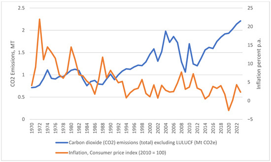
Figure 1. Inflation and CO₂ Emissions. Source: World Development Indicators, World Bank.

The current setup links inflation to CO₂ emissions from an ecological macroeconomics perspective (Fontana & Sawyer, 2016; Rezai & Stagl, 2016). Ecological macroeconomics, as a field, studies the economy as a subsystem of the Earth’s finite ecological system and emphasizes how growth, production, and consumption interact with energy use, resource limits, and environmental boundaries (Jackson, 2009; Victor, 2008). This view differs from structural policies that focus on energy substitution, production technologies, and technological shifts. Instead, we report that the negative association between inflation and CO₂ emissions works through demand suppression. This distinction is necessary for asymmetric effects. Neftci (1984) and Caggiano and Maurici (2026) report that economic indicators tend to display asymmetric effects over the different phases of the business cycle. Notably, inflation tends to be higher in expansionary periods, whilst it tends to slow down in recessionary periods. Noting this pattern, ignoring the non-linearity in inflation could lead to a specification bias, hence blurring inference.

To the best of our knowledge, there is no prior country-specific study that explores the nonlinear association between inflation and CO₂ emissions in Fiji. We find that an increase in the consumer price-based inflation rate reduces more strongly than an equivalently sized decrease in the inflation rate increases CO₂ emissions. The Fourier-based causality test indicates unidirectional causality from inflation to CO₂ emissions. We control structural breaks using the recently developed Fourier-based ARDL model, which can model the effects of various structural breaks while mitigating the overfitting problem that arises due to the inclusion of many dummy variables (Banerjee et al., 2017). We model nonlinearities using the partial sum decomposition approach popularized by Shin et al. (2014) and confirm an asymmetric effect of inflation on CO₂ emissions, distinguishing our study from that of Grolleau and Weber (2024). The results are robust to the GDP deflator-based rate of inflation.

Our main contribution lies in documenting an asymmetric inflation–emissions nexus for Fiji. We highlight that the effect of inflation on CO₂ emissions is asymmetric, depending on the direction of change in inflation. We extend the prior work of Grolleau and Weber (2024) by exploring these asymmetric effects and by providing valuable, country-specific evidence on Fiji, a country facing the dual challenges of a cost-of-living crisis and bearing the brunt of climate change. Our findings indicate that aggregate demand appears highly sensitive to real income declines, meaning that rising prices are likely to trigger a disproportionately large contraction in aggregate consumption, which dampens CO₂ emissions in inflationary periods. The findings indicate that price stability, in the form of controlling inflation, may come at the expense of higher CO₂ emissions. Overall, the core contribution of this paper is the evidence of an asymmetric macroeconomic transmission from inflation to CO₂ emissions. Notably, our findings are distinct from and do not imply permanent structural/technological transitions. Rather, the main findings suggest that stabilization policies may face an ecological trade-off.

Second, we highlight the nonlinear moderating role of financial development. We find that positive shocks to financial development accentuate the negative effect of inflation on CO₂ emissions. Negative shocks, by contrast, attenuate the negative effect of inflation on CO₂ emissions. High inflationary environments, coupled with financial sector development, more strongly reduce CO₂ emissions. Better-developed financial systems tighten credit conditions, raise borrowing costs, and reduce loan availability more effectively in this setting, which further constrains household and firm spending and investment. Declines in inflation lead to a smaller increase in CO₂ emissions when financial development stalls. When financial development deteriorates, households and firms have less access to credit and fewer opportunities to borrow or leverage rising real incomes.

In what follows, the rest of the paper is structured as follows: Section 2 presents a review of the relevant literature, Section 3 presents the model and methods, Section 4 presents the data and results, and Section 5 concludes with policy implications and future research.

2. Literature Review and Hypothesis Development

The conceptual framework of this study is mainly rooted in ecological macroeconomics (Fontana & Sawyer, 2016; Rezai & Stagl, 2016). Ecological macroeconomics is a field that studies the economy as a subsystem of the Earth’s finite ecological system rather than something operating in isolation (Fontana & Sawyer, 2016; Rezai & Stagl, 2016). Foundational contributions by Jackson (2009) and Victor (2008) emphasize that macroeconomic models must account for resource constraints, energy throughput, and environmental carrying capacity, moving beyond conventional growth-oriented frameworks. The field focuses on how growth, production, and consumption interact with energy use, resource limits, and environmental boundaries like climate stability and biodiversity (Fontana & Sawyer, 2016; Rezai & Stagl, 2016). It seeks macro-level policies, such as steady-state or post-growth frameworks, that prioritize well-being, ecological sustainability, and resilience over perpetual GDP growth (Fontana & Sawyer, 2016; Rezai & Stagl, 2016).

Within this overarching framework, we posit inflation as a key mechanism that influences emissions by altering relative prices, real incomes, and investment behavior, thereby shaping the consumption and production decisions of households and firms. Household inflation expectations play a crucial role in this transmission mechanism. Duca-Radu et al. (2021) demonstrate that when households expect higher inflation, they may accelerate purchases of durable goods, temporarily boosting consumption and emissions. Similarly, Bachmann et al. (2015) show that inflation expectations significantly influence household spending decisions, particularly for credit-constrained consumers. Firms’ responses to inflation also matter: when faced with rising input costs, firms may adjust production techniques, potentially shifting toward or away from energy-intensive processes (Grolleau & Weber, 2024).

The theoretical mechanisms linking inflation to emissions operate through multiple channels. First, rising prices could compel customers to accelerate purchases of long-standing durable goods, thereby boosting consumption (Duca-Radu et al., 2021). To capitalize on this, firms begin to ramp up production, which raises CO₂ emissions (Grolleau & Weber, 2024). Moreover, when faced with inflationary pressures, customers may substitute costly, environmentally friendly products with cheaper, less environmentally friendly products (Grolleau & Weber, 2024). This substitution incentivizes the production of cheaper, albeit environmentally deleterious products.

The counterargument is that rising prices reduce private spending. This arises because households face a reduction in real income (Erosa & Ventura, 2002; Grolleau & Weber, 2024). Interpreted in this way, inflation is equivalent to a consumption tax, prompting a rise in savings (Heer & Süssmuth, 2009). Erosa and Ventura (2002) provide a rigorous theoretical treatment of inflation as a regressive consumption tax, showing that it disproportionately affects liquidity-constrained households who cannot smooth consumption through financial markets. In this setting, customers may prefer energy-efficient products if price levels are consistently rising (Grolleau & Weber, 2024). A similar argument can be made for companies, which restructure their production techniques and replace older equipment and machines with newer, more energy-efficient alternatives (Grolleau & Weber, 2024). High inflation could also prompt consumers to shift to secondhand goods. Because secondhand goods do not require production, this causes less pollution than new goods (Grolleau & Weber, 2024). A final channel observed by Grolleau and Weber (2024) is the redistribution effects. Inflation tends to increase income inequality, which reduces carbon emissions (Ghossoub & Reed, 2017).

Empirical evidence generally leans towards a negative association. Grolleau and Weber (2024) reaffirm a negative effect of inflation on CO₂ emissions in 189 countries over the period from 1970 to 2020. However, they argue that the observed effect appears too weak to reach recommended CO₂ emission reductions, implying policymakers should focus on alternative sustainability-oriented policies. Ahmad et al.’s (2021) study differs from that of Grolleau and Weber (2024), as they focus on inflation stability. On the inflation expectations and consumption behavior front, household and firm responses to inflation may depend crucially on whether price changes are perceived as temporary or permanent, influencing investment in energy-efficient technologies (Grolleau & Weber, 2024).

Regarding country-specific studies, Khan (2019) examines the relationship between carbon emission, GDP, and financial development in Pakistan using annual data from 1971 to 2016. Khan’s (2019) findings report that macroeconomic instability raises pollution. Khan (2019) recommends the important role of macroeconomic stability in achieving pollution reduction. The case for Pakistan is also considered by Ullah et al. (2020) using annual data from 1975 to 2018. Negative inflation instability shocks reduce CO₂ emissions. Positive shocks are insignificant. Ullah et al. (2020) sum up recommendations for effective policy towards economic stability, being useful for attaining sustainability across the environment and pollution. Similarly, Sisodia et al. (2023) mentioned that sustainability measures, such as carbon sequestration techniques, technological advancement, efficient production techniques, etc., become focus areas for the government, policymakers, and organizations.

Setyadharma et al. (2021) explore this relationship in Indonesia from 1981 to 2017 employing the error correction model (ECM) approach. They report that high inflation is linked to lower emissions in the long run. The study recommends inflation stability as a key indicator for accomplishing environmental progress (Setyadharma et al., 2021). Musarat et al. (2021) test this relationship in the Malaysian construction industry. Specifically, a reduction in inflation reduces building material prices while increasing the value of construction work. They propose a carbon emission calculation framework, which could help industries make effective policy decisions towards carbon emissions and mitigate the effects from large-scale construction firms (Musarat et al., 2021). Shpak et al. (2022) provide evidence of this relationship in the USA and the Asia Pacific regions, covering data from 1970 to 2020. Their analysis confirms that carbon emission is influenced by macroeconomic indicators such as the unemployment index, GDP, and the inflation rate.

However, these studies do not consider the possibility that inflation may have an asymmetric effect on CO₂ emissions. In formulating our main hypothesis, we follow Grolleau and Weber (2024), who report a negative association between inflation and CO₂ emissions. We extend the work of Grolleau and Weber (2024) by arguing that it is plausible that an increase in inflation could reduce emissions more strongly than an equivalently sized decrease in inflation would raise them in Fiji. The asymmetry becomes amplified by the prevalence of hand-to-mouth households: Rao (2007) estimates that around 75% of consumers in Fiji live with little to no savings, a finding corroborated by Nishkar Kumar et al. (2023). Such households are extremely sensitive to real income declines, meaning that rising prices are likely to trigger a disproportionately large contraction in aggregate consumption, which in turn dampens CO₂ emissions in inflationary periods.

On the other hand, a decrease in inflation could raise CO₂ emissions more strongly than an equivalent increase in inflation would reduce them. Given the high share of hand-to-mouth households in Fiji (Rao, 2007; Nishkar Kumar et al., 2023), real income gains from lower inflation are likely to translate rapidly into higher consumption, as liquidity-constrained households have limited capacity to save (Jappelli & Pistaferri, 2010). By contrast, during higher inflation, spending cuts are constrained by the need to maintain essential consumption, implying that emissions cannot fall proportionally. This suggests a stronger emission response to disinflation than to inflation.

Surprisingly, despite being a key economic indicator, existing research on inflation and CO₂ emissions does not consider the nonlinearity inherent in inflation. Among the two competing perspectives on nonlinearity, we argue that the first may be more relevant to Fiji. Because most consumers may be arguably hand-to-mouth (Rao, 2007; Nishkar Kumar et al., 2023), they may respond more strongly to increasing inflation, as this may further constrain their spending power. Nonetheless, the counterargument is also possible: because most consumers are hand-to-mouth, a decrease in inflation would enable them to increase consumption more strongly, potentially leading to an equally strong hike in CO₂ emissions.

Consequently, nested within the overarching ecological macroeconomics perspective is this hand-to-mouth demand suppression mechanism that potentially describes the presence of asymmetries in the relationship between inflation and CO₂ emissions. As a result, this study posits its first hypothesis in the null form below:

H1. 

An increase in inflation reduces CO₂ emissions by the same amount as an equivalently sized reduction in inflation would raise CO₂ emissions.

Financial development may moderate the effect of inflation on CO₂ emissions through its influence on household consumption smoothing. The theoretical foundations for this moderation effect draw from the literature on financial development and household behavior. Levine (2005) provides a comprehensive overview of how financial development facilitates consumption smoothing, risk management, and intertemporal allocation of resources. In more financially developed settings, households have greater access to credit, savings instruments, and formal financial services, which reduces their reliance on current income for consumption (Bauer, 2016; Wang & Chen, 2025). This enables them to smooth spending over time rather than adjusting consumption one-for-one with changes in real income. As a result, in economies with higher financial development, the contraction in consumption during inflationary periods may be less pronounced (Bauer, 2016; Wang & Chen, 2025), thereby weakening the downward effect of inflation on CO₂ emissions.

Conversely, when inflation falls, financially developed households are better able to save or invest real income gains rather than immediately increasing consumption, which may temper the rise in emissions associated with disinflation. However, in financially underdeveloped contexts, such as Fiji, where households are hand-to-mouth (Rao, 2007; Nishkar Kumar et al., 2023), limited access to credit and savings means that consumption reacts more strongly to both inflation and disinflation. Consequently, financial development attenuates the asymmetric consumption response to inflation and, in turn, moderates the relationship between inflation and CO₂ emissions.

The measurement of financial development in developing countries requires careful consideration. Gizaw et al. (2024) argue that financial sector size, measured by liquid liabilities, adequately captures financial development in contexts where capital markets are less developed, and banking sectors dominate financial intermediation. This makes it an appropriate proxy for Fiji, where the financial system remains bank-dominated with limited equity market development.

Consequently, financial development may function as a buffer in the hand-to-mouth mechanism described above. We, therefore, posit hypothesis 2 in the null form below:

H2. 

Financial development does not weaken the asymmetric effect of inflation on CO₂ emissions.

3. Data and Methods

3.1. Data and Model

Following Grolleau and Weber (2024), we begin with the following model to test hypothesis 1:

$$\ln {CO}_{2,t}=\alpha +\eta {INF}_t+\beta {\ln Y}_t+u_t$$

(1)

where ${CO}_2$ is total carbon emissions from the agriculture, energy, waste, and industrial sectors, $INF$ is the consumer price index-based inflation rate, $Y$ is real GDP per capita, and $u_t$ is the error term. We expect inflation to have a non-zero effect on carbon emissions.

All data required to estimate the model are obtained from the World Bank’s World Development Indicators database. We utilize a sample from 1970 to 2023, which amounts to 54 annual observations. The CO₂ measure is an annual measure of carbon dioxide emissions, one of the six Kyoto-protocol greenhouse gas emissions. All estimations are done with the Eviews 10 statistical software, and variables are defined in Table 1.

Table 1. Variable Definitions.

Variable	Description	Source
${CO}_{2,t}$	Total carbon emissions from agriculture, energy, waste, and industrial sectors	WDI
${INF}_t$	Consumer price index-based inflation rate	WDI
${INF\text{\_}DEF}_t$	GDP deflator-based inflation rate	WDI
$Y_t$	Real GDP per capita	WDI
${FD}_t$	Financial development, measured as the natural logarithm of liquid liabilities.	WDI
${ENG}_t$	Total energy consumption	WDI
${LIR}_t$	Lending interest rate	WDI

Source: Author’s own elaboration. Base year for all monetary sums is 2011.

3.2. Fourier Nonlinear ARDL Model

We utilize the Fourier Nonlinear Autoregressive Distributed Lag (FNARDL) model for estimation. The benefit of the FNARDL model is that it is applicable with either I (0) or I (1) data and can identify cointegration in multivariate systems (Banerjee et al., 2017). Moreover, identical lags do not need to be applied to each explanatory variable (Cho et al., 2023).

Importantly, the FNARDL model mitigates the endogeneity problem, provided the residuals are free from serial correlation (Banerjee et al., 2017; Cho et al., 2023). The Fourier function further controls for structural breaks of an unknown number (Banerjee et al., 2017). This is useful because incorporating many structural breaks dummy variables can lead to an overfitting problem (Banerjee et al., 2017). Moreover, it is possible that there may be more than one structural break in any given year, which makes it difficult to ascertain the event a particular break pertains to (Banerjee et al., 2017).

The Fourier Nonlinear ARDL is defined as:

$$\Delta z_t=d\left(t\right)+ {\beta }_3{z}_{t-1}+{\beta }_4{x}_{t-1}+{\sum }_{i=1}^{r-1}{\beta }_{1i}\Delta z_{t-i}+{\sum }_{i=0}^{q-1}{\beta }_{2i}\Delta x_{t-i}+u_t$$

(2)

where:

$$d\left(t\right)={\mu }_1+{\beta }_1\mathit{sin}\left(2\pi \rho t/T\right)+{\beta }_2\mathit{cos}\left(2\pi \rho t/T\right)$$

(3)

and the model follows an ARDL$(r,q)$ structure (Kumar et al., 2019).

The optimal lag length and value of rho ($\rho$) is determined by the Akaike Information Criteria (Banerjee et al., 2017). We use an iterative method to determine the value of rho. We begin by defining upper and lower bounds of rho between 0 and 4 inclusive and identify rho at one decimal place. We then estimate the FNARDL model within these bounds to determine an intermediate value of rho (Banerjee et al., 2017). This process is repeated until convergence is achieved in the value of rho.

We assess the existence of a long-run relationship through the bounds test of cointegration (Pesaran et al., 2001). After estimating Equation (2) by least squares, we implement a test of joint significance on the lagged level variables. Cointegration is observed if the resulting F-statistic exceeds the upper critical bound (Pesaran et al., 2001). A short-run relationship is observed if the resulting F-statistic is below its lower critical bound (Pesaran et al., 2001). An inconclusive outcome is observed if the resulting F-statistic falls within the upper and lower bounds (Pesaran et al., 2001).

We incorporate nonlinearity through partial sum decompositions (Shin et al., 2014):

$$x_t^{+}={\sum }_{j=1}^t\Delta x_t^{+}={\sum }_{j=1}^t\mathrm{m}\mathrm{a}\mathrm{x}(\Delta x_t^{+},0)$$

(4)

and

$$x_t^{-}={\sum }_{j=1}^t\Delta x_t^{-}={\sum }_{j=1}^t\mathrm{m}\mathrm{i}\mathrm{n}(\Delta x_t^{-},0)$$

(5)

where:

$$x_t=x_0+x_t^{+}+x_t^{-}$$

(6)

where the partial sum processes are identified by the “+” and “−” superscripts, which correspond to both positive and negative changes in the test variable (Shin et al., 2014).

Incorporating the partial sum decompositions in Equation (2) yields:

$$\begin{gathered} \Delta z_t=d\left(t\right)+ {\beta }_3{z}_{t-1}+{\beta }_4^{+}{x}_{t-1}^{+}+{\beta }_4^{-}{x}_{t-1}^{-}+{\sum }_{i=1}^{r-1}{\beta }_{1i}\Delta z_{t-i}+{\sum }_{i=0}^{q-1}{\beta }_{2i}\Delta {x_{t-i}}^{+}+ \\ {\sum }_{i=0}^{q-1}{\beta }_{2i}\Delta {x_{t-i}}^{-}+u_t \end{gathered}$$

(7)

where asymmetric effects are confirmed if ${\beta }^{+}\ne {\beta }^{-}$, plausibly suggesting two outcomes, either ${\beta }^{+}>{\beta }^{-}$ or ${\beta }^{-}> {\beta }^{+}$, assuming $x_t$ increases $z_t$. The latter suggests that a decline in $x_t$ more strongly reduces $z_t$ compared to by how much an increase in $x_t$ increases $z_t$. Conversely, where ${\eta }^{+}>{\eta }^{-}$, assuming $x_t$ increases $z_t$, then an increase in $x_t$ more strongly increases $z_t$ compared to by how much a decrease in $x_t$ reduces $z_t$.

The final step of the FNARLDL analysis visually reaffirms the pattern of asymmetric adjustment to the long run via the cumulative dynamic multiplier as follows:

$$m_h^{+}={\sum }_{j=0}^h{\displaystyle \frac{\partial z_{t+j}}{\partial x_t^{+}}}; m_h^{-}={\sum }_{j=0}^h{\displaystyle \frac{\partial z_{t+j}}{\partial x_t^{-}}}, h=\mathrm{0,1},2,$$

(8)

where $m_h^{+}$ and $m_h^{-}$ describe the evolution of the asymmetric coefficients to their long-run values as the horizon approaches infinity ($h\to \infty$). Augmenting the asymmetric ARDL-type analysis, such as the FNARDL model, with dynamic multipliers is crucial because it provides a visual plot that describes the dynamics of how short-run coefficients asymmetrically converge to their long-run counterparts. Asymmetric dynamic multipliers provide important information on the duration of short-run dynamics, which complements the error correction analysis (Shin et al., 2014).

3.3. Fourier Causality Test

Following Alper et al. (2023) and Athari et al. (2025), we assess causality by incorporating the trigonometric terms of the Fourier function into the Toda and Yamamoto (1995) (TY) causality test. This approach identified causality among variables with mixed or fractional orders of integration, even strictly without cointegrated variables (Athari et al., 2025). A further benefit is that it utilizes information on the maximum lag length of the NFARDL model (Athari et al., 2025). Consequently, we specify the following VAR model:

$$z_t=d\left(t\right)+{\sum }_{i=1}^k{\alpha }_{1i}{z}_{t-i}+{\sum }_{j=k+1}^{dmax}{\alpha }_{2j}{z}_{t-j}+{\sum }_{i=1}^k{\alpha }_{3i}{x}_{t-i}+{\sum }_{j=k+1}^{dmax}{\alpha }_{4j}{x}_{t-j}+u_{1t}$$

(9)

and

$$x_t=d\left(t\right)+{\sum }_{i=1}^k{\beta }_{1i}{z}_{t-i}+{\sum }_{j=k+1}^{dmax}{\beta }_{2j}{z}_{t-j}+{\sum }_{i=1}^k{\beta }_{3i}{x}_{t-i}+{\sum }_{j=k+1}^{dmax}{\beta }_{4j}{x}_{t-j}+u_{1t}$$

(10)

where d(t) is defined earlier.

We establish causality from x to z if the combined coefficient of all the lags of x is statistically significant (Athari et al., 2025). Reliability of the causality test is assessed through the inverse roots of the characteristic polynomial (Athari et al., 2025). The VAR model is assessed as stable if the inverse roots lie within the unit circle.

4. Results

4.1. Descriptive Statistics and Correlation Matrix

Table 1 presents the descriptive statistics and correlation matrix of the key variables in this study. Regarding the baseline explanatory variables, inflation appears negatively correlated with CO₂ emissions. Real GDP per capita appears positively correlated (Table 2). The correlations with additional controls and moderating variables also appear high with CO₂ emissions.

Table 2. Descriptive Statistics and Correlation Matrix.

Statistics	$\mathbf{ln}{\mathit{C}\mathit{O}}_{2,\mathit{t}}$	${\mathit{I}\mathit{N}\mathit{F}}_{\mathit{t}}$	${\mathit{I}\mathit{N}\mathit{F}\text{\_}\mathit{D}\mathit{E}\mathit{F}}_{\mathit{t}}$	${\mathbf{ln}\mathit{Y}}_{\mathit{t}}$	${\mathit{F}\mathit{D}}_{\mathit{t}}$	${\mathbf{ln}\mathit{E}\mathit{N}\mathit{G}}_{\mathit{t}}$	${\mathit{L}\mathit{I}\mathit{R}}_{\mathit{t}}$
Panel A. Descriptive statistics
Mean	0.1955	5.4217	5.6893	8.9817	21.9433	22.5577	7.8618
Median	0.1445	4.2963	3.6840	8.9550	21.9298	22.5616	7.4778
Maximum	0.7932	21.978	29.645	9.3704	23.0894	23.0167	12.4500
Minimum	−0.3386	−2.5952	−4.7198	8.6091	20.7928	22.0627	4.9707
Std. Dev.	0.3145	4.3554	6.0093	0.1891	0.6627	0.2624	2.1276
Skewness	0.1895	1.3731	1.8527	0.3732	0.0736	−0.0880	0.7165
Kurtosis	1.9516	5.6414	7.5772	2.4574	1.8119	1.7670	2.3967
Jarque–Bera	2.7959	32.667 A	78.034 A	1.9164	3.2246	2.7145	3.2233
	[0.2470]	[<0.01]	[<0.01]	[0.3835]	[0.1994]	[0.2574]	[0.1995]
Panel B. Correlation matrix
$\ln {CO}_{2,t}$	1.0000
	-
${INF}_t$	−0.5541 A	1.0000
	[<0.01]	-
${INF\text{\_}DEF}_t$	−0.3514 A	0.6734 A	1.0000
	[<0.01]	[<0.01]	-
${\ln Y}_t$	0.9018 A	−0.5490 A	−0.3870 A	1.0000
	[<0.01]	[<0.01]	[<0.01]	-
${FD}_t$	0.8577 A	−0.6515 A	−0.4953 A	0.9147	1.000000
	[<0.01]	[<0.01]	[<0.01]	[<0.01]	-
${\ln ENG}_t$	0.9470 A	−0.2363	−0.2905	0.6220 A	0.5997 A	1.000000
	[<0.01]	[0.2087]	[0.1194]	[<0.01]	[<0.01]	-
${LIR}_t$	−0.7457 A	0.2599	0.1072	−0.8691 A	−0.8199 A	−0.7521 A	1.000000
	[<0.01]	[0.1654]	[0.5729]	[<0.01]	[<0.01]	[<0.01]	-

Note: ^A—indicates normally distributed in Panel A and significant correlation in Panel B. p-value in [.]. Sample for Ln ENG is 42 observations from 1980 to 2021. Sample for LIR is 32 observations from 1992 to 2023. A common sample is used for correlation analysis.

4.2. Unit Root and Cointegration and Asymmetric Effects

Table 3 presents the unit root test results. We employ the group-based Levin–Lin–Chu test, which pools the variables together and assumes a common unit root process. We also rely on Im–Pesaran–Shin unit root test, the Fisher augmented Dickey–Fuller, and Fisher–Phillips–Perron tests, which, although they pool the variables together, assume an individual unit root process. The unit root test results indicate that the variables are integrated into order 1 and are therefore suitable for estimation with the FNARDL approach.

Table 3. Unit Root Tests.

Method	Statistic	Prob.	Cross-Sections	Obs.
Panel A. Levels
LLC: common unit root process	−0.9481	0.1641	7	224
IPS W-stat: individual unit root process	−0.8244	0.2091	7	224
ADF-Fisher Chi-sq: individual unit root process	9.8996	0.1327	7	224
PP-Fisher Chi-sq: individual unit root process	9.3516	0.1547	7	224
Panel B. First differences
LLC: common unit root process	−9.1306 A	<0.01	7	224
IPS W-stat: individual unit root process	−9.8912 A	<0.01	7	224
ADF-Fisher Chi-sq: individual unit root process	85.1001 A	<0.01	7	224
PP-Fisher Chi-sq: individual unit root process	105.011 A	<0.01	7	224

Note: ^A—stationarity at 1 percent. Source: Author’s estimation in Eviews 10. LLC: Levin–Lin–Chu test, IPS: Im–Pesaran–Shin test.

Subsequently, we present the results of the bounds test of cointegration based on Pesaran et al. (2001) in Table 4 below. We note the presence of cointegration at the 1 percent level in the nonlinear models. This conclusion holds when either asymptotic bounds from Pesaran et al. (2001) or finite sample bounds from Narayan (2005) are considered. Finally, we present the results of the WALD test exploring whether inflation has asymmetric effects on CO₂ emissions in Table 5. We confirm asymmetric effects in the long run and short run.

Table 4. Cointegration.

Test Statistic	Value	Sig.	Asymptotic: n = 1000		Finite Sample: n = 50
			Lower Bound	Upper Bound	Lower Bound	Upper Bound
F-statistic	7.6085 A	10%	2.37	3.2	2.538	3.398
		5%	2.79	3.67	3.048	4.002
		1%	3.65	4.66	4.188	5.328

Note: ^A—cointegration at 1 percent. Asymptotic bounds based on Pesaran et al. (2001). Finite sample bounds based on Narayan (2005).

Table 5. Asymmetric Effects Test.

Test Statistic	Test Statistic	Degrees of Freedom	Prob.
Panel A. Long-run (Null: Long-run symmetry)
t-statistic	−2.6615 B	37	0.0114
F-statistic	7.0840 B	(1, 37)	0.0114
Chi-square	7.0840 A	1	0.0078
Panel B. Short-run (Null: Short-run symmetry)
t-statistic	−2.8432 A	37	0.0072
F-statistic	8.0838 A	(1, 37)	0.0072
Chi-square	8.0838 A	1	0.0045

Note: ^A, ^B—asymmetry at 1 and 5 percent level.

4.3. Long-Run and Short-Run

We present the results of the long-run and short-run models in Table 6 below. We note that an increase in inflation reduces CO₂ emissions more strongly than a decrease in inflation increases CO₂ emissions. The error correction term is appropriately signed and is significant. The short-run results indicate that positive shocks of inflation increase CO₂ emissions, whereas negative shocks are insignificant. These results suggest that rising inflation further tightens budget constraints of the largely hand-to-mouth consumers in Fiji, leading to a sharp decrease in consumption, hence reducing CO₂ emissions.

Table 6. Long-run and Short-run Results.

Variable	Coefficient	Std. Error	t-Statistic	Prob.
Panel A. Short run
$\Delta {INF}_t^{+}$	−0.0105	0.0100	−1.0492	0.3009
$\Delta {INF}_{t-1}^{+}$	−0.0068	0.0119	−0.5694	0.5725
$\Delta {INF}_{t-2}^{+}$	0.0177 C	0.0097	1.8193	0.0770
$\Delta {INF}_{t-3}^{+}$	0.0171 B	0.0075	2.2744	0.0288
$\Delta {INF}_t^{-}$	−0.0125	0.0121	−1.0256	0.3117
${\Delta \ln Y}_t$	1.0118 A	0.2156	4.6929	0.0000
$\mathit{cos}\left(2\pi \rho t/T\right)$	−0.0226	0.0186	−1.2167	0.2314
$\mathit{sin}\left(2\pi \rho t/T\right)$	−0.0554 B	0.0207	−2.6699	0.0112
${ECT}_{t-1}$	−0.6231 A	0.1004	−6.2056	0.0000
Panel B. Long-run
${INF}_t^{+}$	−0.0760 A	0.0204	−3.7220	0.0007
${INF}_t^{-}$	−0.0667 A	0.0165	−4.0280	0.0003
${\ln Y}_t$	1.6236 A	0.3059	5.3074	0.0000
$\mathit{cos}\left(2\pi \rho t/T\right)$	−0.0363	0.0305	−1.1920	0.2408
$\mathit{sin}\left(2\pi \rho t/T\right)$	−0.0890 A	0.0303	−2.9338	0.0057
Intercept	−14.0613 A	2.5898	−5.4293	0.0000

Note: ^A, ^B, ^C—significant at 1, 5, and 10 percent. Maximum lag length and optimum lag specification of the ARDL structure, and optimal rho value of 3.9 of the Fourier frequency is based on AIC.

Our findings differ from those of Grolleau and Weber (2024) because we explicitly show that inflation has asymmetric effects on CO₂ emissions in the long run and short run. While we agree with Grolleau and Weber (2024) that there is a negative association between inflation and CO₂ emissions, we extend their work by incorporating asymmetric effects in the analysis. We argue that ignoring the asymmetries inherent in inflation is likely to lead to specification issues.

The pattern of asymmetric effects is reaffirmed by the dynamic multiplier (Figure 2). The dynamic multiplier value converges with its long-run values, suggesting robust results. Moreover, we note that the FNARDL estimates are free from specification issues, the residual terms are not serially correlated, the residual variances are not heteroscedastic, and the error terms appear normally distributed (Table 7). The CUSUM and CUSUMSQ plots support model stability (Figure 3).

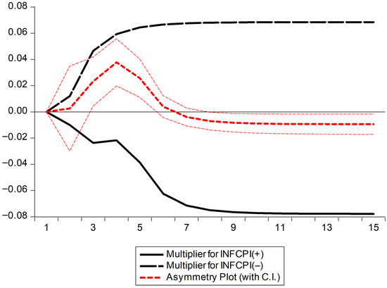
Figure 2. Dynamic Asymmetric Multiplier. Note: Figure 2 presents the asymmetrical plot for unit shocks in inflation.

Table 7. FNARDL Diagnostic Test Results.

Test	Null Hypothesis	Degrees of Freedom	Chi-SQ Test Statistic
Breusch–Godfrey	No serial correlation	2	4.5662 [0.1020]
Breusch–Pagan–Godfrey	No heteroscedasticity	11	3.2349 [0.9872]
Jarque–Bera	Residual normality	1	2.2591 [0.3232]
Ramsey RESET	Correct functional form	1	0.0417 [0.8393]

Note: p-value in [.].

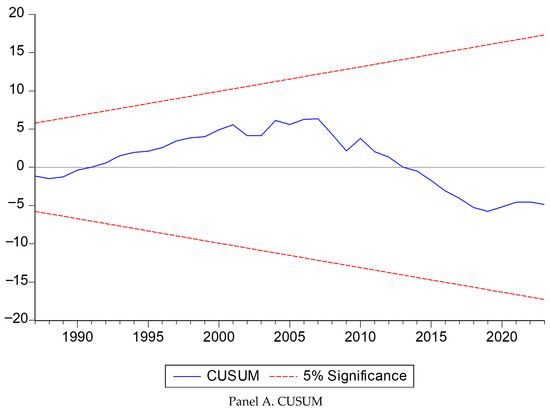
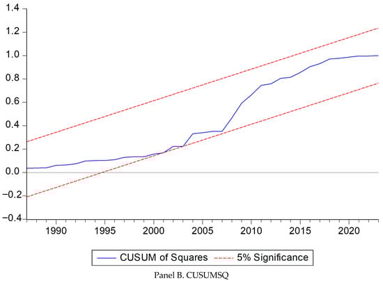
Figure 3. CUSUM and CUSUMSQ Stability Plots. Note: CUSUM and CUSUMSQ plots within 5 percent critical bounds indicate stable estimates.

4.4. Fourier TY Causality

We utilize a lag of 2 for the causality assessment, which is within the maximum lag of 4 for the ARDL analysis. The Fourier TY causality results indicate unidirectional causality from inflation to carbon emissions (Table 8). The causality outcome is supportive of our baseline results. The inverse roots of the characteristic polynomial fall within the unit circle, suggesting the test VAR is stable, and causality results are reliable (Figure 4).

Table 8. Fourier Causality Results—Significant Results Only.

Causal Direction	Chi-SQ Test Statistic	Degrees of Freedom	Prob.
${INF}_t^{+}\to \ln {CO}_{2,t}$	4.9545 C	2	0.0840
${INF}_t^{-}\to \ln {CO}_{2,t}$	9.2070 B	2	0.0100
${INF}_t^{-}\to {INF}_t^{+}$	11.1304 A	2	0.0038
${INF}_t^{+}\to {INF}_t^{-}$	35.1587 A	2	0.0000

Note: ^A, ^B, ^C—causality at 1, 5, and 10 percent.

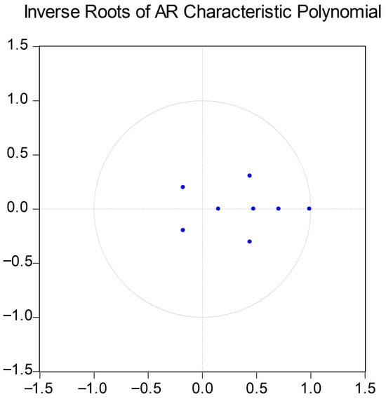
Figure 4. Inverse Roots Characteristic Polynomial Plots. Note: Inverse roots characteristic polynomial plots within unit circle indicate stable VAR.

4.5. Robustness Tests

We consider four sensitivity tests. First, we replace the CPI-based inflation rate with the GD deflator-based inflation rate. We note consistent results, with the identical pattern of asymmetric effects, after estimating with the NFARDL model. This suggests that the results are not driven by a particular measure of inflation (Table 9). This insight is crucial because although the CPI and GDP-deflator-based inflation rates generally mirror each other (Figure 5), the CPI focuses on consumer prices paid for a basket of goods, whereas the GDP deflator measures the average change in prices of all goods and services produced domestically. While the CPI is better used for tracking the cost of living, it remains widely used in studies on the effects of inflation (Grolleau & Weber, 2024). The GDP-deflator-based results satisfy the various diagnostic tests, are cointegrated at 1 percent, and generally produce stable results.

Table 9. Long-run and Short-run Results: GDP Deflator.

Variable	Coefficient	Std. Error	t-Statistic	Prob.
Panel A. Cointegrating Form
$\Delta {INF\text{\_}DEF}_t^{+}$	0.0080	0.0066	1.2202	0.2320
$\Delta {INF\text{\_}DEF}_{t-1}^{+}$	0.0018	0.0079	0.2265	0.8222
$\Delta {INF\text{\_}DEF}_{t-2}^{+}$	−0.0027	0.0074	−0.3852	0.7028
$\Delta {INF\text{\_}DEF}_{t-3}^{+}$	0.0108 C	0.0057	1.8823	0.0694
$\Delta {INF\text{\_}DEF}_t^{-}$	−0.0122 B	0.0054	−2.2613	0.0311
$\Delta {INF\text{\_}DEF}_{t-1}^{-}$	0.0012	0.0061	0.1961	0.8458
$\Delta {INF\text{\_}DEF}_{t-2}^{-}$	0.0057	0.0056	1.0252	0.3134
$\Delta {INF\text{\_}DEF}_{t-3}^{-}$	0.0074	0.0046	1.6088	0.1181
$\Delta {\ln Y}_t$	0.9004 A	0.2676	3.3642	0.0021
$\Delta {\ln Y}_{t-1}$	−0.3675	0.3823	−0.9613	0.3441
$\Delta {\ln Y}_{t-2}$	0.2358	0.4330	0.5446	0.5900
$\Delta {\ln Y}_{t-3}$	−0.1773	0.3295	−0.5380	0.5945
$\mathit{cos}\left(2\pi \rho t/T\right)$	−0.0592 A	0.0214	−2.7606	0.0097
$\mathit{sin}\left(2\pi \rho t/T\right)$	−0.0299	0.0245	−1.2206	0.2317
${ECT}_{t-1}$	−0.5764 A	0.1184	−4.8684	0.0000
Panel B. Long Run Coefficients
${INF\text{\_}DEF}_t^{+}$	−0.0428 B	0.0167	−2.5530	0.0160
${INF\text{\_}DEF}_t^{-}$	−0.0393 B	0.0146	−2.6843	0.0117
${\ln Y}_t$	1.6377 A	0.4042	4.0514	0.0003
$\mathit{cos}\left(2\pi \rho t/T\right)$	−0.1027 B	0.0387	−2.6525	0.0126
$\mathit{sin}\left(2\pi \rho t/T\right)$	−0.0519	0.0390	−1.3312	0.1931
Intercept	−14.3473 A	3.3612	−4.2684	0.0002

Note: ^A, ^B, ^C—significant at 1, 5, and 10 percent levels. Maximum lag length and optimum lag specification of the ARDL structure, and optimal rho value of 3.9 of the Fourier frequency is based on AIC.

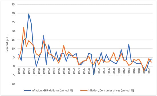
Figure 5. CPI and GDP-deflator-based Inflation Rates. Source: World Development Indicators, World Bank.

Second, we consider an alternative estimation methodology in the form of the dynamic least squares (DOLS) approach (Stock & Watson, 1993). The benefits of this approach are that it corrects for endogeneity in the cointegrating vector by including leads and lags of first differenced regressors (Masih & Masih, 1996). Moreover, by including leads and lags, DOLS mitigates the effect of serially correlated residuals (Masih & Masih, 1996). Unlike traditional least squares, DOLS provides unbiased and consistent estimates even in small samples (Masih & Masih, 1996). Additionally, its small sample properties make DOLS an attractive alternative to methods such as FMOLS, which rely on asymptotic properties (Phillips & Hansen, 1990). We note that the DOLS results and pattern of asymmetric effects are qualitatively identical to the Fourier-based NARDL model (Table 10).

Table 10. Long-run results: DOLS.

Variable	Coefficient	Std. Error	t-Statistic	Prob.
${INF}_t^{+}$	−0.0491 B	0.0197	−2.4866	0.0185
${INF}_t^{-}$	−0.0393 B	0.0146	−2.6474	0.0126
${\ln Y}_t$	1.5752 A	0.3466	4.5443	0.0001
$\mathit{cos}\left(2\pi \rho t/T\right)$	−0.0353	0.0325	−1.0864	0.3857
$\mathit{sin}\left(2\pi \rho t/T\right)$	−0.0759 B	0.0316	−2.4013	0.0225
Intercept	−13.7229 A	2.9683	−4.6232	0.0001

Note: ^A, ^B—significant at 1 and 5 percent levels. Model assumes a lead of 1, lag of 2, with Newey–West standard errors, pre-whitened with 1-lag with a Bartlett kernel. Optimal rho value of 3.9 based on AIC.

A further robustness test considered attempts to alleviate the issue of omitted variables. For instance, energy usage is likely to correlate with CO₂ emissions due to the use of fossil fuels. Moreover, inflation is likely to be impacted by monetary policy indicators because the overarching goal of monetary policy is price stability (Kumar et al., 2025)1. As a result, we include these additional control variables in our analysis. Table 11 indicates that these results, which include energy consumption and the lending interest rate, are consistent with our baseline results. We reiterate that our baseline results do not suffer from omitted variables based on the Ramsey RESET test (Table 7).

Table 11. FARDL omitted variables robustness test.

Variable	Coefficient	Std. Error	t-Statistic	Prob.
Panel A. Cointegrating Form
$\Delta {INF}_t^{+}$	−0.304489 A	0.005746	−52.987756	0.0000
$\Delta {INF}_{t-1}^{+}$	0.212586 A	0.003745	56.762470	0.0000
$\Delta {INF}_t^{-}$	−0.008976 B	0.003841	−2.336810	0.0361
$\Delta {INF}_{t-1}^{-}$	−0.017895 A	0.005671	−3.155326	0.0076
$\Delta {\ln Y}_t$	0.023889	0.161140	0.148251	0.8844
$\Delta {\ln Y}_{t-1}$	0.007615	0.136059	0.055971	0.9562
$\Delta {\ln ENG}_t$	0.002128	0.069047	0.030821	0.9759
$\Delta {\ln ENG}_{t-1}$	0.079812	0.046115	1.730696	0.1072
$∆{LIR}_t$	1.506349 A	0.012096	124.533778	0.0000
$\mathit{cos}\left(2\pi \rho t/T\right)$	1.048654 A	0.009787	107.150735	0.0000
$\mathit{sin}\left(2\pi \rho t/T\right)$	−1.404495 A	0.016600	−84.610440	0.0000
${ECT}_{t-1}$	−0.661406 A	0.178487	−3.705625	0.0026
Panel B. Long Run Coefficients
${INF}_t^{+}$	−0.157789 A	0.036839	−4.283245	0.0009
${INF}_t^{-}$	−0.046283 A	0.009435	−4.905274	0.0003
${\ln Y}_t$	−0.072306	0.186758	−0.387165	0.7049
${\ln ENG}_t$	−0.108379	0.218460	−0.496102	0.6281
${LIR}_t$	2.277497	0.623254	3.654203	0.0029
$\mathit{cos}\left(2\pi \rho t/T\right)$	1.585493	0.428377	3.701161	0.0027
$\mathit{sin}\left(2\pi \rho t/T\right)$	−2.123501	0.555997	−3.819264	0.0021
Intercept	−1.554962	4.688251	−0.331672	0.7454

Note: ^A, ^B—significant at 1, 5 percent levels. Maximum lag length and optimum lag specification of the ARDL structure, and optimal rho value of 3.9 of the Fourier frequency is based on AIC.

The final robustness checks further attempt to correct for endogeneity using the two-stage least squares approach. We use up to two lags of the continuous explanatory variables, excluding the trigonometric terms as instruments for the analysis. We note that the results are similarly signed and are quantitatively similar to our baseline estimates (Table 12). The Durbin–Hausman endogeneity test indicates that the regressors do not suffer from the endogeneity bias (p-value = 0.66, with a null hypothesis of exogeneity).

Table 12. Long-run results: 2SLS.

Variable	Coefficient	Std. Error	t-Statistic	Prob.
${INF}_t^{+}$	−0.008572 B	0.003594	−2.283624	0.0271
${INF}_t^{-}$	−0.008208 B	0.003582	−2.393007	0.0208
${\ln Y}_t$	1.333457 A	0.200139	6.662641	0.0000
$\mathit{cos}\left(2\pi \rho t/T\right)$	−0.033903 A	0.008355	−4.058033	0.0002
$\mathit{sin}\left(2\pi \rho t/T\right)$	−0.050316 A	0.016044	−3.136074	0.0030
Intercept	−11.78760 A	2.9683	−4.6232	0.0001
Regressor Endogeneity Test: Null: All continuous variables are exogenous. Test stat. = 1.5691, p-value = 0.6664

Note: ^A, ^B—significant at 1, 5 percent levels. Newey–West standard errors, pre-whitened with 1-lag with a Bartlett kernel. Optimal rho value of 3.9 adopted from baseline estimates.

4.6. Tests on Moderating Role of Financial Development: Hypothesis 2

To test hypothesis 2, we specify the following long-run model

$$\ln {CO}_{2,t}=\alpha +{\eta }^{+}{INF}_t^{+}+{\eta }^{-}{INF}_t^{-}+{\zeta }^{+}{INF}_t^{+}{FD}_t^{+}+{\zeta }^{-}{INF}_t^{-}{FD}_t^{-}+\beta {\ln Y}_t+u_t$$

(11)

where the marginal effect of positive/negative inflationary shocks on CO₂ emissions is:

$${\displaystyle \raisebox{1ex}{$\partial \ln {CO}_{2,t}$}\!\left/ \!\raisebox{-1ex}{$\partial {INF}_t^{+}$}\right.}={\eta }^{+}+{\zeta }^{+}{FD}_t^{+}$$

(12)

and

$${\displaystyle \raisebox{1ex}{$\partial \ln {CO}_{2,t}$}\!\left/ \!\raisebox{-1ex}{$\partial {INF}_t^{-}$}\right.}={\eta }^{-}+{\zeta }^{-}{FD}_t^{-}$$

(13)

where positive financial development shocks accentuate the effect of positive inflationary shocks on CO₂ emissions if ${\eta }^{+}$ and ${\zeta }^{+}$ have the same signs, and vice versa. The same logic applies to negative inflationary and financial development shocks. Note that Equation (12) also includes the standalone effect of the positive and negative shocks of financial development to correctly identify marginal effects2.

To maintain directional consistency between the independent variables and the moderator, we interact positive inflationary shocks with positive financial development shocks. Using total financial development would mix opposing effects from positive and negative shocks, creating an incongruence problem that could obscure the asymmetric moderation effect. We measure financial development using the natural logarithm of liquid liabilities. Gizaw et al. (2024) argue that financial sector size adequately measures financial development in developing countries, where capital markets are less developed, and banking sectors dominate financial intermediation. This characterization accurately describes countries such as Fiji.

4.6.1. Theoretical Rationale for Including Both Real GDP and Financial Development

In the ecological macroeconomics literature, real GDP per capita captures the scale effect—the proposition that larger economic output generates more emissions through increased production and consumption (Grossman & Krueger, 1995; Copeland & Taylor, 2004). Financial development, by contrast, captures the composition and technique effects—how the structure of the financial system influences credit constraints, investment behavior, and the adoption of cleaner technologies (Tamazian et al., 2009; Shahbaz et al., 2013).

Omitting either variable would conflate distinct theoretical mechanisms central to our analysis. If we excluded real GDP, any estimated moderating effect of financial development could simply reflect omitted income effects rather than the genuine financial sector influences on consumption smoothing and credit constraints that we theorize in Section 2. Specifically, our hand-to-mouth consumer framework (Rao, 2007; Nishkar Kumar et al., 2023) requires controlling for income to isolate the additional constraining effect of financial sector conditions on liquidity-constrained households.

Thus, while multicollinearity inflates standard errors—making hypothesis tests more conservative—the theoretical imperative to include both variables outweighs the efficiency loss. As Kennedy (2008, p. 193) notes, “multicollinearity is a data deficiency problem, not a statistical problem,” and the appropriate response is transparent acknowledgment rather than omission of theoretically justified variables.

We present the variance inflation factors (VIF) of the estimated FARDL model, including financial development. We note that the mean VIF of real GDP per capita is 3.09, which is less than the threshold of 5. We note that the mean VIF of the positive shocks of financial development is 3.48, and that of negative shocks is 10.64. The VIFs are presented in differences because ARDL models are estimated via unconstrained error correction models (Cho et al., 2023).

4.6.2. Moderation Results

The moderation results indicate that positive financial development shocks accentuate the negative effect of positive inflationary shocks on CO₂ emissions (Table 13). This suggests that high inflationary environments, coupled with financial sector development, more strongly reduce CO₂ emissions. Better-developed financial systems tighten credit conditions, raise borrowing costs, and reduce loan availability more effectively, which further constrains household and firm spending and investment. This may deepen the contraction in energy use and production, thereby strengthening the decline in CO₂ emissions when inflation rises.

Table 13. Variance Inflation Factors—Moderation Model.

Variable	VIF
$\Delta \ln {CO}_{2,t}$	6.3166
$\Delta \ln {CO}_{2,t-1}$	4.4996
$\Delta \ln {CO}_{2,t-2}$	3.1561
$\Delta {INF}_t^{+}$	5.8201
$\Delta {INF}_{t-1}^{+}$	4.1590
$\Delta {INF}_{t-2}^{+}$	4.2277
$\Delta {INF}_{t-3}^{+}$	8.6099
$\Delta {INF}_t^{-}$	7.3932
$\Delta {INF}_{t-1}^{-}$	10.9450
$\Delta {INF}_{t-2}^{-}$	14.0453
${\Delta \ln Y}_t$	2.5131
${\Delta \ln Y}_{t-1}$	2.6652
${\Delta \ln Y}_{t-2}$	4.1095
$\Delta {FD}_t^{+}$	4.7660
$\Delta {FD}_{t-1}^{+}$	3.1285
$\Delta {FD}_{t-2}^{+}$	2.5459
$\Delta {FD}_t^{-}$	18.1554
$\Delta {FD}_{t-1}^{-}$	3.1223
$\mathit{cos}\left(2\pi \rho t/T\right)$	3.9001
$\mathit{sin}\left(2\pi \rho t/T\right)$	7.2188

In contrast, negative financial development shocks weaken the negative association between negative inflationary shocks and CO₂ emissions. In other words, declines in inflation lead to a smaller increase in CO₂ emissions when financial development stalls. When financial development deteriorates, households and firms have less access to credit and fewer opportunities to borrow or leverage rising real incomes. As a result, even when inflation falls, liquidity constraints prevent a strong consumption and investment rebound, which dampens the increase in energy use and CO₂ emissions.

Nonetheless, the correlation matrix presented in Table 2 suggests a very high correlation between financial development and real GDP. Including these two variables in the same regression model could lead to inflated standard errors and destabilized coefficients. For this reason, we reassess whether financial development moderates the effect of inflation on CO₂ emissions after omitting the natural log of real GDP from the specification. We note that the pattern of asymmetric effects occurred for both tests (Table 14 and Table 15).

Table 14. FARDL Moderation Results: Standalone and Moderating Effects of Financial Development.

Variable	Coefficient	Std. Error	t-Statistic	Prob.
Panel A. Long Run
${INF}_t^{+}$	−0.092482 A	0.020118	−4.596965	0.0002
${INF}_t^{-}$	−0.103553 A	0.019022	−5.443786	0.0000
${\ln Y}_t$	0.159379	0.344474	0.462674	0.6486
${FD}_t^{+}$	−1.353546 A	0.405424	−3.338591	0.0033
${FD}_t^{-}$	1.728789	1.566237	1.103785	0.2828
${INF}_t^{+}\times {FD}_t^{+}$	−0.002131	0.005587	−0.381506	0.7069
${INF}_t^{-}\times {FD}_t^{-}$	0.085731 B	0.030566	2.804835	0.0109
$\mathit{cos}\left(2\pi \rho t/T\right)$	0.050434 B	0.023656	2.131955	0.0456
$\mathit{sin}\left(2\pi \rho t/T\right)$	−0.202660 A	0.030854	−6.568256	0.0000
Intercept	−0.330031	3.197564	−0.103213	0.9188
Panel B. Short Run
$\Delta \ln {CO}_{2,t}$	0.104363	0.132511	0.787579	0.4402
$\Delta \ln {CO}_{2,t-1}$	−0.200126 C	0.110456	−1.811823	0.0851
$\Delta \ln {CO}_{2,t-2}$	0.212586 B	0.092443	2.299645	0.0324
$\Delta {INF}_t^{+}$	−0.008976	0.010388	−0.864070	0.3978
$\Delta {INF}_{t-1}^{+}$	−0.017895 C	0.009965	−1.795784	0.0877
$\Delta {INF}_{t-2}^{+}$	−0.023889 B	0.010059	−2.374917	0.0277
$\Delta {INF}_{t-3}^{+}$	0.064098 A	0.009049	7.083487	0.0000
$\Delta {INF}_t^{-}$	−0.007615	0.011877	−0.641210	0.5287
$\Delta {INF}_{t-1}^{-}$	−0.006001	0.010022	−0.598847	0.5560
$\Delta {INF}_{t-2}^{-}$	0.079812 A	0.012651	6.308739	0.0000
${\Delta \ln Y}_t$	1.048654 A	0.207902	5.043985	0.0001
${\Delta \ln Y}_{t-1}$	−1.506349 A	0.286548	−5.256884	0.0000
${\Delta \ln Y}_{t-2}$	1.02846 A	0.291007	3.534139	0.0021
$\Delta {FD}_t^{+}$	−1.185458 A	0.307605	−3.853836	0.0010
$\Delta {FD}_{t-1}^{+}$	0.375747	0.275529	1.363731	0.1878
$\Delta {FD}_{t-2}^{+}$	0.404694 C	0.224666	1.801316	0.0868
$\Delta {FD}_t^{-}$	3.017752 B	1.149302	2.625727	0.0162
$\Delta {FD}_{t-1}^{-}$	2.537563 A	0.476619	5.324096	0.0000
$\Delta {INF}_t^{+}\times \Delta {FD}_t^{+}$	−0.001632	0.004176	−0.390799	0.7001
$\Delta {INF}_t^{-}\times \Delta {FD}_t^{-}$	0.065650 A	0.018213	3.604494	0.0018
$\mathit{cos}\left(2\pi \rho t/T\right)$	0.038621 C	0.020063	1.925004	0.0686
$\mathit{sin}\left(2\pi \rho t/T\right)$	−0.155191 A	0.027573	−5.628263	0.0000
${ECT}_{t-1}$	−0.765768 A	0.138880	−5.513904	0.0000

Note: ^A, ^B, ^C—significant at 1, 5, and 10 percent levels. Lag specification and optimal rho value adopted from baseline estimates.

Table 15. FARDL Moderation Results: Standalone and Moderating Effects of Financial Development excluding real GDP.

Variable	Coefficient	Std. Error	t-Statistic	Prob.
Panel A. Long run
${INF}_t^{+}$	−0.056341 A	0.019525	−2.885610	0.0091
${INF}_t^{-}$	−0.068587 A	0.012479	−5.496297	0.0000
${FD}_t^{+}$	−1.197943 A	0.365812	−3.274749	0.0038
${FD}_t^{-}$	1.016983	1.751663	0.580581	0.5680
${INF}_t^{+}\times {FD}_t^{+}$	−0.004716	0.006020	−0.783423	0.4426
${INF}_t^{-}\times {FD}_t^{-}$	0.083799 B	0.029523	2.838417	0.0102
$\mathit{cos}\left(2\pi \rho t/T\right)$	0.022330	0.024226	0.921732	0.3677
$\mathit{sin}\left(2\pi \rho t/T\right)$	−0.210105 A	0.026047	−8.066429	0.0000
Intercept	0.953822 A	0.230336	4.141012	0.0005
Panel B. Short run
$\Delta \ln {CO}_{2,t}$	0.243086	0.175691	1.383597	0.1817
$\Delta \ln {CO}_{2,t-1}$	−0.061918	0.141770	−0.436753	0.6670
$\Delta \ln {CO}_{2,t-2}$	0.277150 B	0.123001	2.253229	0.0356
$\Delta {INF}_t^{+}$	−0.012278	0.014587	−0.841723	0.4099
$\Delta {INF}_{t-1}^{+}$	−0.025706 B	0.011779	−2.182395	0.0412
$\Delta {INF}_{t-2}^{+}$	−0.004355	0.011915	−0.365528	0.7186
$\Delta {INF}_{t-3}^{+}$	0.044321 A	0.010406	4.259089	0.0004
$\Delta {INF}_t^{-}$	0.024978 C	0.012154	2.055076	0.0532
$\Delta {INF}_{t-1}^{-}$	0.023062 C	0.011333	2.034844	0.0553
$\Delta {INF}_{t-2}^{-}$	0.049364 A	0.012704	3.885777	0.0009
$\Delta {INF}_{t-3}^{-}$	0.011295	0.007295	1.548275	0.1372
$\Delta {FD}_t^{+}$	−1.220604 B	0.457925	−2.665511	0.0149
$\Delta {FD}_{t-1}^{+}$	−0.513196	0.360376	−1.424056	0.1698
$\Delta {FD}_{t-2}^{+}$	1.356975 A	0.349452	3.883151	0.0009
$\Delta {FD}_{t-3}^{+}$	−0.693600 B	0.286276	−2.422832	0.0250
$\Delta {FD}_t^{-}$	4.129463 A	1.151069	3.587502	0.0018
$\Delta {FD}_{t-1}^{-}$	2.532536 A	0.751950	3.367959	0.0031
$\Delta {FD}_{t-2}^{-}$	−1.842153 B	0.727279	−2.532938	0.0198
$\Delta {FD}_{t-3}^{-}$	1.976731 A	0.645807	3.060872	0.0062
$\Delta {INF}_t^{+}\times \Delta {FD}_t^{+}$	−0.004387	0.005058	−0.867494	0.3960
$\Delta {INF}_t^{-}\times \Delta {FD}_t^{-}$	0.077958 A	0.019079	4.086016	0.0006
$\mathit{cos}\left(2\pi \rho t/T\right)$	0.020773	0.024433	0.850200	0.4053
$\mathit{sin}\left(2\pi \rho t/T\right)$	−0.195461 A	0.040362	−4.842686	0.0001
${ECT}_{t-1}$	−0.930301 A	0.180774	−5.146223	0.0000

Note: ^A, ^B, ^C—significant at 1, 5, and 10 percent levels. Lag specification and optimal rho value adopted from baseline estimates.

5. Conclusions, Policy Implications, Limitations, and Further Research

This paper explores the asymmetric effect of inflation on CO₂ emissions using Fiji as a case study from 1970 to 2023. Notably, prior research does not explore this issue within the Fijian context. We base our study on a research hypothesis that explores the potential of asymmetric effects. Utilizing the Fourier Nonlinear Autoregressive Distributed Lag (FNARDL) model, we find that an increase in inflation reduces CO₂ emissions more strongly than a reduction in inflation raises CO₂ emissions. The results imply that rising inflation may tighten budget constraints of mostly hand-to-mouth consumers in Fiji (Rao, 2007), leading to a sharp decrease in consumption, hence reducing CO₂ emissions (Grolleau & Weber, 2024). This demand suppression mechanism is distinct from supply-oriented factors such as technological innovation and clean energy substitution. It offers evidence on the sustainability implications of inflation, providing monetary policymakers, whose primary goal is price stability, with knowledge of the potential ecological implications of their stabilization policy initiatives.

The findings point to a non-trivial policy trade-off between macroeconomic stabilization and environmental sustainability. While inflation can reduce CO₂ emissions by suppressing carbon-intensive economic activity, relying on inflation as an implicit environmental policy instrument is neither socially nor economically optimal (Grolleau & Weber, 2024). Persistently high inflation erodes real incomes, disproportionately affects low-income households, and undermines welfare by reducing purchasing power and living standards (Grolleau & Weber, 2024). Thus, inflation-driven emission reductions should be viewed as a by-product of economic conditions rather than a deliberate climate policy tool.

The moderating role of financial development further highlights the importance of financial sector strength and stability in achieving sustainability goals. Positive financial development shocks amplify the emission-reducing effects of inflation. Better-developed financial systems tighten credit conditions, thereby constraining household spending and investment, thereby strengthening the decline in CO₂ emissions when inflation rises. Declines in inflation lead to a smaller increase in CO₂ emissions when financial development slows down. When financial development weakens, households and firms have less access to credit and fewer opportunities to borrow or leverage rising real incomes. As a result, even when inflation falls, liquidity constraints prevent a strong consumption rebound, which weakly raises CO₂ emissions.

A limitation of our study is the presence of multicollinearity in the moderation analysis, as evidenced by the correlation matrix given in Table 2 and the VIF values given in Table 13. This multicollinearity arises from the strong conceptual and empirical correlation between financial development and income: a well-documented relationship in development economics (Levine, 2005). While multicollinearity does not bias coefficient estimates, it inflates standard errors, making statistical inference more conservative (Wooldridge, 2015).

Another potential limitation relates to omitted variables. We have attempted to mitigate the influence of omitted variables in our analysis by including energy consumption and the lending interest rate. While these return significant results, we note that our baseline conclusions do not change. We further note that the Ramsey RESET test indicates that our baseline model does not suffer from omitted variables. We further note that our Fourier-based nonlinear ARDL model is a specific type of ARDL model that incorporates nonlinearity and structural break analysis through the Fourier function. ARDL models may mitigate the endogeneity bias, provided the residuals are free from serial correlation (Cho et al., 2023). Nonetheless, structural endogeneity due to omitted variables could persist. Moreover, the causality analysis, while showing that the dataset exhibits unidirectional causality from inflation to CO₂ emissions, emissions could plausibly affect inflation through energy prices, production costs, and supply-side constraints. While ARDL models may mitigate endogeneity, we have attempted to mitigate the issue of omitted variables by considering additional control variables. We supplement our analysis using the two-stage least squares and dynamic least squares methods and note consistent results.

Based purely on the results, Fijian policymakers contemplating stabilization policy should recognize the ecological implications of inflation. A high inflationary environment suppresses demand, which reduces CO₂ emissions. This becomes more pronounced with high financial development, as with an inflationary environment, more developed financial markets can better restrict the availability of credit, which further constrains aggregate spending behavior. Monetary tightening, therefore, may help mitigate CO₂ emissions.

However, this demand suppression mechanism must not serve as a substitute for structural policies, e.g., the deployment of energy-efficient technologies, and other such decarbonization programs. Therefore, inflation should not be treated as an environmental policy tool. Future research could explore how inflation may contribute to such technological and structural policies on sustainability. What the current study does show is that stabilization policy, especially monetary policy, due to its focus on price stability, should recognize inflation’s carbon emission implications. Governments could consider energy relief packages to help ease cost-of-living burdens.

Future research could extend this analysis by examining alternative greenhouse gases such as methane (CH₄) and nitrous oxide (N₂O), which have higher global warming potential than CO₂, to better capture the environmental effects of inflation. Although this study provides a useful foundation for understanding the ecological implications of macroeconomic indicators in climate-vulnerable countries like Fiji, future work could use higher-frequency data to incorporate additional controls and improve robustness. Researchers might also explore this methodology in other small island developing states and developing economies to assess external validity and investigate country-specific structural factors and global external shocks. Panel data in nonlinear frameworks could further examine whether financial development moderates the inflation–emissions nexus while strengthening identification through improved instrumentation.

References

- Ahmad, W., Ullah, S., Ozturk, I., & Majeed, M. T. (2021). Does inflation instability affect environmental pollution? Fresh evidence from Asian economies. Energy & Environment, 32(7), 1275–1291. [Google Scholar] [CrossRef]
- Alper, A. E., Alper, F. O., Ozayturk, G., & Mike, F. (2023). Testing the long-run impact of economic growth, energy consumption, and globalization on ecological footprint: New evidence from Fourier bootstrap ARDL and Fourier bootstrap Toda–Yamamoto test results. Environmental Science and Pollution Research, 30(15), 42873–42888. [Google Scholar] [CrossRef] [PubMed]
- Athari, S. A., Addia, K., Kirikkaleli, D., Al Geitany, S. H., Al Fadhel, L., & Saliba, C. (2025). Do environmental taxes and green electricity matter for environmental quality? Fresh evidence in France based on Fourier methods. Energies, 18(19), 5046. [Google Scholar] [CrossRef]
- Bachmann, R., Berg, T. O., & Sims, E. R. (2015). Inflation expectations and readiness to spend: Cross-sectional evidence. American Economic Journal: Economic Policy, 7(1), 1–35. [Google Scholar] [CrossRef]
- Banerjee, P., Arčabić, V., & Lee, H. (2017). Fourier ADL cointegration test to approximate smooth breaks with new evidence from crude oil market. Economic Modelling, 67, 114–124. [Google Scholar] [CrossRef]
- Bauer, S. (2016). Does credit access affect household income homogeneously across different groups of credit recipients? Evidence from rural Vietnam. Journal of Rural Studies, 47, 186–203. [Google Scholar] [CrossRef]
- Briguglio, L. (1995). Small island developing states and their economic vulnerabilities. World Development, 23(9), 1615–1632. [Google Scholar] [CrossRef]
- Caggiano, E., & Maurici, F. (2026). Gone with the cycle: The asymmetric impact of business cycle on growth. The Journal of Economic Asymmetries, 33, e00447. [Google Scholar] [CrossRef]
- Campbell, J. Y., & Mankiw, N. G. (1989). Consumption, income, and interest rates: Reinterpreting the time series evidence. NBER Macroeconomics Annual, 4, 185–216. [Google Scholar] [CrossRef]
- Chanel, A. (2025). Can we tackle Fiji’s cost of living crisis? The Fiji Times. Available online: https://www.fijitimes.com.fj/opinion-can-we-tackle-fijis-cost-of-living-crisis/ (accessed on 5 January 2026).
- Cho, J. S., Greenwood-Nimmo, M., & Shin, Y. (2023). Recent developments of the autoregressive distributed lag modelling framework. Journal of Economic Surveys, 37(1), 7–32. [Google Scholar] [CrossRef]
- Copeland, B. R., & Taylor, M. S. (2004). Trade, growth, and the environment. Journal of Economic Literature, 42(1), 7–71. [Google Scholar] [CrossRef]
- Duca-Radu, I., Kenny, G., & Reuter, A. (2021). Inflation expectations, consumption and the lower bound: Micro evidence from a large multi-country survey. Journal of Monetary Economics, 118, 120–134. [Google Scholar] [CrossRef]
- Erosa, A., & Ventura, G. (2002). On inflation as a regressive consumption tax. Journal of Monetary Economics, 49(4), 761–795. [Google Scholar] [CrossRef]
- Fontana, G., & Sawyer, M. (2016). Towards post-Keynesian ecological macroeconomics. Ecological Economics, 121, 186–195. [Google Scholar] [CrossRef]
- Ghossoub, E. A., & Reed, R. R. (2017). Financial development, income inequality, and the redistributive effects of monetary policy. Journal of Development Economics, 126, 167–189. [Google Scholar] [CrossRef]
- Gizaw, T., Getachew, Z., & Mancha, M. (2024). Financial development and economic growth: Evidence from emerging African and Asian countries. Cogent Economics & Finance, 12(1), 2398213. [Google Scholar] [CrossRef]
- Grolleau, G., & Weber, C. (2024). The effect of inflation on CO2 emissions: An analysis over the period 1970–2020. Ecological Economics, 217, 108029. [Google Scholar] [CrossRef]
- Grossman, G. M., & Krueger, A. B. (1995). Economic growth and the environment. The Quarterly Journal of Economics, 110(2), 353–377. [Google Scholar] [CrossRef]
- Heer, B., & Süssmuth, B. (2009). The savings-inflation puzzle. Applied Economics Letters, 16(6), 615–617. [Google Scholar] [CrossRef]
- Jackson, T. (2009). Prosperity without growth: Economics for a finite planet. Routledge. [Google Scholar]
- Jappelli, T., & Pistaferri, L. (2010). The consumption response to income changes. Annual Review of Economics, 2(1), 479–506. [Google Scholar] [CrossRef]
- Kennedy, P. (2008). A guide to econometrics (6th ed.). Blackwell Publishing. [Google Scholar]
- Khan, M. (2019). Does macroeconomic instability cause environmental pollution? The case of Pakistan economy. Environmental Science and Pollution Research, 26(14), 14649–14659. [Google Scholar] [CrossRef]
- Kumar, N. N., Bibi, K., & Mohnot, R. (2025). From boom to bust: Unravelling the cyclical nature of Fiji’s money demand. Journal of Risk and Financial Management, 18(7), 381. [Google Scholar] [CrossRef]
- Kumar, N. N., Kumar, R. R., Patel, A., & Stauvermann, P. J. (2019). Exploring the effect of tourism and economic growth in Fiji: Accounting for capital, labor, and structural breaks. Tourism Analysis, 24(2), 115–130. [Google Scholar] [CrossRef]
- Levine, R. (2005). Finance and growth: Theory and evidence. In P. Aghion, & S. N. Durlauf (Eds.), Handbook of economic growth (Vol. 1, pp. 865–934). Elsevier. [Google Scholar] [CrossRef]
- Long, H., Prasad, B., Krishna, V., Tang, K., & Chang, C. P. (2024). Understanding the key determinants of Fiji’s renewable energy. Economic Analysis and Policy, 82, 1144–1157. [Google Scholar] [CrossRef]
- Masih, R., & Masih, A. M. (1996). Stock-Watson dynamic OLS (DOLS) and error-correction modelling approaches to estimating long-and short-run elasticities in a demand function: New evidence and methodological implications from an application to the demand for coal in mainland China. Energy Economics, 18(4), 315–334. [Google Scholar] [CrossRef]
- Musarat, M. A., Alaloul, W. S., Liew, M. S., Maqsoom, A., & Qureshi, A. H. (2021). The effect of inflation rate on CO2 emission: A framework for Malaysian construction industry. Sustainability, 13(3), 1562. [Google Scholar] [CrossRef]
- Narayan, P. K. (2005). The saving and investment nexus for China: Evidence from cointegration tests. Applied Economics, 37(17), 1979–1990. [Google Scholar] [CrossRef]
- Neftci, S. N. (1984). Are economic time series asymmetric over the business cycle? Journal of Political Economy, 92(2), 307–328. [Google Scholar] [CrossRef]
- Nishkar Kumar, N., Patel, A., Shalendra Prasad, N., & Nandani, S. (2023). Loss aversion or hand-to-mouth behaviour in private consumption models. New Zealand Economic Papers, 57(3), 247–259. [Google Scholar] [CrossRef]
- Pesaran, M. H., Shin, Y., & Smith, R. J. (2001). Bounds testing approaches to the analysis of level relationships. Journal of Applied Econometrics, 16(3), 289–326. [Google Scholar] [CrossRef]
- Phillips, P. C. B., & Hansen, B. E. (1990). Statistical inference in instrumental variables regression with I(1) processes. The Review of Economic Studies, 57(1), 99–125. [Google Scholar] [CrossRef]
- Rao, B. B. (2007). Estimating short and long-run relationships: A guide for the applied economist. Applied Economics, 39(13), 1613–1625. [Google Scholar] [CrossRef]
- Read, R. (2004). The implications of increasing globalization and regionalism for the economic growth of small island states. World Development, 32(2), 365–378. [Google Scholar] [CrossRef]
- Rezai, A., & Stagl, S. (2016). Ecological macroeconomics: Introduction and review. Ecological Economics, 121, 181–185. [Google Scholar] [CrossRef]
- Setyadharma, A., Oktavilia, S., Wahyuningrum, I. F. S., Nikensari, S. I., & Saputra, A. M. (2021). Does inflation reduce air pollution? Evidence from Indonesia. E3S Web of Conferences, 317, 01068. [Google Scholar] [CrossRef]
- Shahbaz, M., Tiwari, A. K., & Nasir, M. (2013). The effects of financial development, economic growth, coal consumption and trade openness on CO2 emissions in South Africa. Energy Policy, 61, 1452–1459. [Google Scholar] [CrossRef]
- Shin, Y., Yu, B., & Greenwood-Nimmo, M. (2014). Modelling asymmetric cointegration and dynamic multipliers in a nonlinear ARDL framework. In Festschrift in honor of Peter Schmidt: Econometric methods and applications (pp. 281–314). Springer New York. [Google Scholar] [CrossRef]
- Shpak, N., Ohinok, S., Kulyniak, I., Sroka, W., Fedun, Y., Ginevičius, R., & Cygler, J. (2022). CO2 emissions and macroeconomic indicators: Analysis of the most polluted regions in the world. Energies, 15(8), 2928. [Google Scholar] [CrossRef]
- Sisodia, G. S., Sah, H. K., Kratou, H., Mohnot, R., Ibanez, A., & Gupta, B. (2023). The long-run effect of carbon emission and economic growth in European countries: A computational analysis through vector error correction model. International Journal of Energy Economics and Policy, 13(3), 271–278. [Google Scholar] [CrossRef]
- Stock, J. H., & Watson, M. W. (1993). A simple estimator of cointegrating vectors in higher order integrated systems. Econometrica, 61(4), 783–820. [Google Scholar] [CrossRef]
- Tamazian, A., Chousa, J. P., & Vadlamannati, K. C. (2009). Does higher economic and financial development lead to environmental degradation? Energy Policy, 37(1), 246–253. [Google Scholar] [CrossRef]
- Toda, H. Y., & Yamamoto, T. (1995). Statistical inference in vector autoregressions with possibly integrated processes. Journal of Econometrics, 66(1–2), 225–250. [Google Scholar] [CrossRef]
- Ullah, S., Apergis, N., Usman, A., & Chishti, M. Z. (2020). Asymmetric effects of inflation instability and GDP growth volatility on environmental quality in Pakistan. Environmental Science and Pollution Research, 27(25), 31892–31904. [Google Scholar] [CrossRef] [PubMed]
- Victor, P. A. (2008). Managing without growth: Slower by design, not disaster. Edward Elgar Publishing. [Google Scholar] [CrossRef]
- Wang, Y., & Chen, Y. (2025). Digital financial inclusion and rural household debt risks. International Journal of Finance & Economics. Available online: https://onlinelibrary.wiley.com/doi/abs/10.1002/ijfe.70028 (accessed on 5 January 2026).
- Wooldridge, J. M. (2015). Introductory econometrics: A modern approach. Nelson Education. [Google Scholar]
Disclaimer/Publisher’s Note: The statements, opinions and data contained in all publications are solely those of the individual author(s) and contributor(s) and not of MDPI and/or the editor(s). MDPI and/or the editor(s) disclaim responsibility for any injury to people or property resulting from any ideas, methods, instructions or products referred to in the content. |
© 2026 by the authors. Licensee MDPI, Basel, Switzerland. This article is an open access article distributed under the terms and conditions of the Creative Commons Attribution (CC BY) license.