When Tracking Error Misleads: Risk Exposure Differences Between ETFs and Their Indices

Abstract

We investigate the underlying risk exposures of ETFs compared with their indices using a Principal Component Analysis approach. Then, we test whether ETFs’ tracking errors can capture the risk exposure difference between ETFs and their underlying benchmarks. We document a significant positive relation between tracking error and differences in risk exposure between ETFs and their corresponding indices. Even modest increases in tracking error are associated with economically meaningful divergences in risk exposure between an ETF and its benchmark. These findings suggest that comparisons of tracking error across index ETFs when making investment decisions may be misleading for investors seeking benchmark-consistent risk exposure.

1. Introduction

Recent years have witnessed a significant expansion of the creation and trading of Exchange-Traded Funds (ETFs). Introduced in the early 1990s, today ETFs provide a diversified investment vehicle for individuals or entities regarding types of assets or geographical focus. By the end of 2024, total net assets in index ETFs amounted to USD 8.1 trillion, representing 23.9% of overall fund market net assets, compared with 8% at the end of 20081. Index ETFs represent a form of passive investment, where managers seek to track rather than outperform a benchmark, contrasting with active management strategies that aim to generate excess returns or alpha (Lettau & Madhavan, 2018). Passive investment strategies rest on the principle of market efficiency, which suggests that investors are unlikely to consistently outperform the market over the long term. Consequently, the primary objective is to replicate overall market performance (Fraś & Rogowski, 2016). The ETFs’ growth comes at the expense of traditional active mutual funds (Stambaugh, 2014). This expansion has encouraged fund managers to develop ETFs with diverse investment objectives and tracking methodologies, resulting in an extensive array of options for investors.

Index ETFs aim to replicate the performance of a specific index or benchmark, offering investors high liquidity, low transaction costs, and a transparent means to achieve broad market exposure. Therefore, the extent to which each ETF replicates its underlying index represents a performance evaluation criterion for investors (Yadav & Pope, 1994; Chu, 2011). The industry standard for measuring this tracking performance is tracking error (hereafter TE), which measures the consistency with which a fund follows its benchmark (Hougan, 2015). Frino and Gallagher (2001), among others, argue that TE is equal to the volatility or standard deviation of the difference between a portfolio’s return and its benchmark index’s return, and is thus a measure of the relative risk of the fund. However, the measurement of TE, in isolation, provides limited interpretive value. The TE only measures the volatility and does not express whether the return differential is positive or negative. Investors tend to compare a particular TE to another one. The lower the tracking error, the more consistently the fund’s return volatility matches that of the benchmark over time. Also, as a rule of thumb, a TE that is closer to zero is better than one that is farther away from zero. Mathematically and empirically, this can be shown with ease. However, we question how close to zero a TE must be to be considered close, and how far from zero is deemed too far. The TE can partially explain the performance of ETFs, as it is unavoidable and necessary (Dorocáková, 2017). We understand that not all index ETFs perfectly replicate their benchmarks because some indices are more difficult to track accurately. Replicating a benchmark involves costs, and in certain situations, legal and regulatory restrictions may prevent an ETF from fully replicating its index (Madhavan, 2016). Additionally, the expense ratio and transaction costs are significant factors that impact TE (Frino & Gallagher, 2001; Saunders, 2018). These drawbacks of TE, among others, motivate this study.

We relate two independent strands of literature to propose a novel approach for assessing ETFs’ performance: fund performance evaluation and factor models. In standard asset pricing frameworks, expected returns are determined by exposure to systematic risk factors; otherwise, rational investors would hold only riskless assets (Ang, 2014). Under the CAPM, the asset’s covariance with the market portfolio drives expected returns, while subsequent work extends this insight to multiple common risk factors (Chen et al., 1986; Fama & French, 2015, among others). In the context of delegated portfolio management, Carhart (1997) shows that fund performance reflects exposure to these common factors as well as implementation costs such as expenses and transaction costs. Applied to index-tracking ETFs, this framework implies that funds that replicate their benchmarks less efficiently should exhibit systematic deviations in risk exposure and, consequently, different risk premia than those that closely track their indices. Kim et al. (2023) document that ETFs with different replication strategies have systematically different tracking errors. Accordingly, we hypothesize that ETFs with low tracking error should display factor exposures similar to those of their underlying indices, whereas higher tracking error may reflect meaningful divergence in underlying risk.

This raises two key considerations for investors: how to compare TEs across ETFs, and what threshold of TE deviation should reasonably be regarded as excessive. We primarily aim to investigate the underlying risk exposures of ETFs compared with their indices. Then, we further investigate whether TEs can capture this risk exposure difference. Finally, we highlight the implications of TE variability for ETFs’ returns relative to their benchmarks.

We employ two samples, daily and weekly, of US equity ETFs. Both samples span the time period from January 2013 to December 2018. We begin by finding the TEs for each ETF. The tracking errors tend to be low overall, with means of around 0.0332 annualized (daily sample) and 0.0224 annualized (weekly sample). Then, we run a Principal Component Analysis (PCA) test based on index variations for each year to assess ETFs’ and indices’ risk exposure to variations in index returns. We relate the risk exposure of each ETF to that of its underlying index by computing the R² difference. The R² difference represents the risk exposure difference between each ETF and its index. We find that a high percentage of variations in ETFs and indices can indeed be explained cross-sectionally by the systemic risk of indices at each particular year. Then, we sort the ETFs in each year according to their TEs, reporting the absolute R² differences. We show that, for both samples, ETFs with the highest TEs exhibit greater variations (gaps) in the differences R² values. The pattern persists through each year of our analysis. Thus, we establish that, not surprisingly, a high TE results in a greater difference in risk exposure between ETFs and their respective indices. Importantly, it is surprising how the TEs’ comparability led to a substantial increase in risk exposure differences. In our weekly sample, we find that ETFs in the highest quartile (fourth) of the yearly mean TE exhibits higher R² differences (21.517–66.416%) than ETFs in the median (third) quartile of the yearly TE (0.314–0.943%). The same pattern is apparent in our daily sample as well. Our results suggest that ETFs with a slightly higher TE have a wider risk exposure difference relative to their benchmarks. Therefore, we argue that comparing TEs across ETFs and assessing the differences between them could lead to higher risk exposure than one would expect by simply measuring the differences in TEs for different ETFs.

To further investigate the relationship between the TEs and risk differences, we repeat our analysis of the TE and R² differences and record monthly variables. Then, we analyze the TEs as the dependent variable, regressed on the absolute R² difference and control variables. We document a statistically significant relationship between the TE and the absolute R² differences at the 1% level. These results support the premise that even slight variations in TEs can significantly impact the risk exposure of ETFs. Therefore, assessing ETF risk by comparing TE differences across ETFs is not as accurate as one would assume. This suggests that investors should exercise caution when comparing TEs across ETFs to make informed investment decisions.

The contributions of this paper are twofold. First, it advances the general literature on index fund performance evaluation, with a particular focus on ETFs. We extend the existing literature on the determinants of TE and focus on measuring TE in a way that reflects investors’ real risk exposure rather than mechanical index deviations. Second, this paper enriches the well-established literature on factor models by enhancing the understanding of their application in evaluating ETF risk and performance, challenging the conventional assumption that a lower tracking error implies a closer alignment with the benchmark in both return and risk.

The remainder of this paper is organized as follows: Section 2 provides an overview of related studies. Section 3 describes the sample and presents the TEs. In Section 4, we investigate the relationship between TEs and ETFs’ risk exposure in depth. Section 5 presents the conclusion.

2. Related Literature Review and Hypothesis Development

Exchange-Traded Funds (ETFs) and index mutual funds share many similarities, as both are designed to replicate the performance of a chosen index and may experience some degree of tracking error relative to their underlying benchmarks. In both cases, investors bear operating expenses that slightly reduce returns (Poterba & Shoven, 2002). However, important structural differences exist between the two vehicles. Unlike index mutual funds, ETFs are traded on exchanges throughout the day, allowing investors to buy, sell, purchase on margin, or sell short. Because ETF trading occurs through brokerage firms, investors may also incur commission fees. Mutual fund transactions, by contrast, are executed only at the end of the trading day at net asset value. Investors in index mutual funds often face higher costs, including management fees, transaction charges, and tax-related expenses (Kostovetsky, 2003). These distinctions suggest that the relative attractiveness of ETFs and index funds depends largely on investor preferences, cost sensitivity, and tax brackets. From a performance perspective, both vehicles are passive investment strategies and therefore limit risk exposure to the index being tracked. Investors in such funds generally expect minimal tracking error. While index investing is the most common form of passive investing, ETFs typically offer lower expense ratios than index mutual funds, and both are substantially less costly than actively managed mutual funds. Given these features, our analysis focuses specifically on the tracking error of ETFs.

2.1. Measurements of the Tracking Error

Roll (1992) provides the foundational economic interpretation of tracking error by showing that, once a benchmark is fixed, portfolio choice is naturally expressed regarding benchmark-relative expected returns and variance, with tracking error serving as the relevant measure of risk. In this setting, positive tracking error is optimal only if it is intentionally assumed in exchange for higher expected benchmark-relative performance. Although this framework was developed in the context of active portfolio management, it offers a point of reference for evaluating passive investment vehicles such as ETFs, which are not intended to generate alpha.

Empirically, there are several popular methods to calculate the tracking error. The ones proposed by Grinold and Kahn (1999); Frino and Gallagher (2001); Aber et al. (2009); Cremers and Petajisto (2009); and Madhavan (2016) are, to our knowledge, the most common. Each of these methods produces a static value representing the TE for a specific period. Importantly, the interpretation of a TE value as a measure of risk does not have a meaning by itself and must be compared with another ETF’s TE. Madhavan (2016) states that the tracking error does not indicate how closely the longer-term performance of the ETF has matched its underlying index. Additionally, he notes that the standard calculation of the tracking error overlooks substantial contributions to ETF performance, such as income from securities lending. Shin and Soydemir (2010) find that tracking errors are persistent and statistically different from zero. They find that ETFs underperform their benchmark indices on a risk-adjusted basis, which is consistent with the presence of tracking errors, and that the change in the exchange rate is a contributor to tracking error. Bae and Kim (2020) find that liquidity affects how closely ETFs track their benchmark indices and that illiquid ETFs tend to have larger tracking errors, greater volatility, and different return patterns compared with more liquid ETFs. Therefore, tracking error, when measured as the standard deviation of the return difference between the ETF returns and the index returns, reflects liquidity risk and arbitrage frictions, not active portfolio choice. Recent studies find that the design and structural features of ETFs affect the tracking error (Kim et al., 2023; Tzioumis & Barbopoulos, 2025).

The above studies suggest that how tracking error is measured is critical. A mismeasured tracking error may understate or mischaracterize the benchmark-relative risk that investors actually bear. Therefore, our study focuses on measuring tracking error in a way that reflects investors’ real risk exposure rather than mechanical index deviations.

2.2. Risk Factor Analysis

Investors in risky assets earn premiums as compensation for potential losses during adverse times, as they are exposed to the underlying risk factors of these assets. The first theory in asset pricing is the Capital Asset Pricing Model (CAPM), formulated in the 1960s by Treynor (1961), Sharpe (1964), Lintner (1965), and Mossin (1966), which predicts that assets that crash with the market are risky, and therefore, they must pay high premiums. Otherwise, rational investors will invest in riskless assets (Ang, 2014). Under the CAPM, only one factor drives expected returns: the asset’s covariance with the market portfolio. Carhart (1997) argues that mutual fund performance is explained by common factors in stock returns, expense ratios, and transaction costs. In this sense, ETFs that mimic a specific index less efficiently should have higher risk premiums than those that closely track the index. Linking this idea to ETFs’ tracking errors, we expect to find ETFs with very low TEs to be exposed to risk factors similar to those the underlying index is exposed to. Assets’ cross-sectional returns are generally considered a bundle of risk factors (Chen et al., 1986; Fama & French, 2015). Therefore, we adopt this approach to evaluate the underlying risk of ETFs relative to their index returns. Kozak et al. (2018) use the standard PCA to investigate the interpretation of risk factors. Specifically, they question whether risk factors are rational or behavioral factors and whether they can be distinguished. Their empirical work shows an important conclusion. They find evidence that cross-sectional variations in expected returns can be explained by a low-dimensional factor analysis (very few factors). They argue that due to the commonality of asset returns and the absence of near-arbitrage opportunities, there is no clear distinction between factors based on risk exposure and behavior-based factors. They conclude that the threshold for identifying behavioral factors is too high (they must be orthogonal to common factors) because risk and behavioral factors are most likely to be highly correlated. Therefore, in this study, we argue that risk factors extracted from index returns should not only explain the ETF’s underlying risk but also provide a sufficient representation of the ETF’s investment risk relative to the universe of indices. We extract the underlying risk factors from index returns, compare the risk exposure of ETFs and their corresponding indices, and relate the underlying risk differences to the TEs.

Empirical evidence shows that ETFs that diverge more from their benchmarks regarding liquidity and underlying risk exposures exhibit higher TEs (e.g., Bae & Kim, 2020), which is consistent with the idea that larger differences in risk exposure should be reflected in greater TE. This raises a central question: does comparing TEs across ETFs provide an accurate assessment of an ETF’s risk exposure relative to its benchmark? In particular, can small differences in TE mask economically meaningful differences in exposure to underlying risk factors?

We hypothesize that even modest increases in TE can expose investors to risk factors beyond those present in the benchmark. This distinction is economically important because it could heavily impact investors’ ability to achieve their investment goals.

3. The Samples and Tracking Errors

3.1. Data

We obtained ETF and index data from the Eikon database (DataStream). For this study, we chose ETFs that are exposed only to US markets, as the underlying risk factors tend to be more homogeneous than in a sample that includes ETFs from international markets. This increases the explanatory power of risk factors. Furthermore, for the same reason, we focused the analysis on equity ETFs. However, the study could also be applicable to non-US ETFs and all types of indexed funds. We then chose ETFs that satisfy the following criteria:

• Indexed ETFs, where the main objective of their fund managers is to mimic a particular index;
• Non-leveraged ETFs that mimic the underlying indices one-to-one, as leveraged ETFs aim to multiply or invert the performance of the underlying index.

The sample includes all ETFs that satisfy the criteria, and their financial data are available on DataStream. The benchmarks from Datastream were matched with the prospectuses of each ETF. The final sample includes 259 ETFs that mimic 239 indices. The data span the time period from the beginning of 2013 until the end of 2018.

The choice of 2013 as the starting point for the sample was motivated by the availability of data and the fact that approximately 23% of the ETFs that meet the criteria are listed after 2013. We use daily and weekly samples. Daily data tend to be noisy (as we observe in the analysis in the coming sections). However, the choice of weekly data limits the noise. The sample includes ETFs from 11 different industries based on the Eikon database classification.

Table 1 reports the sample distribution by industry, with about one-third of ETFs concentrated in the financial sector. However, we do not expect this concentration to introduce significant bias, as our analysis includes both ETFs and their underlying indices, ensuring that the risk factors account for both. Additionally, the primary goal of indexed ETFs is to mimic their benchmark indices.

Table 1. Sample distribution by industry.

Industries	Number of ETFs
Financials	84
Technology	52
Non-Classified Equity *	34
Cyclical Consumer Goods and Services	19
Industrial	17
Energy	15
Healthcare	15
Basic Materials	9
Non-Cyclical Consumer Goods and Services	7
Utilities	6
Telecommunication Services	1
Total	259

* Equity-based ETFs that tend to cover broader industries. This table shows the sample distribution of ETFs over the period from 2013 to 2018, classified by industry. We obtained the ETF data from the Thomson Reuters Eikon database (Datastream).

3.2. Tracking Errors and the Underlying Risk Factors

3.2.1. Tracking Error

As noted, passive managers aim to replicate an index. Therefore, if an ETF is managed “perfectly,” its return, on average, equals the dollar return of the index. Passive managers have no incentive to take additional risks to outperform the index. Therefore, large deviations of ETF returns from the index do not serve the best interests of investors.

If an ETF perfectly mirrors its underlying index, the TE should be zero. Among the methods previously discussed for calculating TE, we chose to follow the methodology of Cremers and Petajisto (2009) because it is rigorous and tends to produce more conservative results. We adapted Cremers and Petajisto’s (2009) methodology to calculate the TEs using time series regressions. We regress the return of each ETF on the return of its benchmark in each time period, and then we determine the value of the TE by calculating the standard deviation of the error term, as follows:

$${\mathrm{R}}_{{\mathrm{E}\mathrm{T}\mathrm{F}}_{\mathrm{i},\mathrm{t}}}={\mathsf{\alpha }}_{\mathrm{E}\mathrm{T}\mathrm{F}}+{\mathsf{\beta }}_{\mathrm{E}\mathrm{T}\mathrm{F}}{\mathrm{R}}_{{\mathrm{I}\mathrm{n}\mathrm{d}\mathrm{e}\mathrm{x}}_{\mathrm{i},\mathrm{t}}}+{\mathsf{\epsilon }}_{\mathrm{E}\mathrm{T}{\mathrm{F}}_{\mathrm{i},\mathrm{t}}}$$

(1)

$$\mathrm{T}\mathrm{r}\mathrm{a}\mathrm{c}\mathrm{k}\mathrm{i}\mathrm{n}\mathrm{g} \mathrm{E}\mathrm{r}\mathrm{r}\mathrm{o}\mathrm{r}\left(\mathrm{T}\mathrm{E}\right)=\mathrm{S}\mathrm{t}.\mathrm{D}\mathrm{e}\mathrm{v}\left[{\mathsf{\epsilon }}_{\mathrm{E}\mathrm{T}{\mathrm{F}}_{\mathrm{i},\mathrm{t}}}\right]$$

(2)

where ${\mathrm{R}}_{{\mathrm{E}\mathrm{T}\mathrm{F}}_{\mathrm{i},\mathrm{t}}}$ is ETF (i) return at time (t), and ${\mathrm{R}}_{{\mathrm{I}\mathrm{n}\mathrm{d}\mathrm{e}\mathrm{x}}_{\mathrm{i},\mathrm{t}}}$ is index (i) return at time (t). The tracking error is the standard deviation of the error term in Equation (1). The ETF and index returns are calculated as the natural log of the first difference at each point in time.

$${\mathrm{R}}_{{\mathrm{E}\mathrm{T}\mathrm{F}}_{\mathrm{i},\mathrm{t}}}=\ln \left({\mathrm{E}\mathrm{T}\mathrm{F}}_{\mathrm{i},\mathrm{t}}\right)-\ln \left({\mathrm{E}\mathrm{T}\mathrm{F}}_{\mathrm{i},\mathrm{t}-1}\right)$$

(3)

$${\mathrm{R}}_{{\mathrm{I}\mathrm{n}\mathrm{d}\mathrm{e}\mathrm{x}}_{\mathrm{i},\mathrm{t}}}=\ln \left({\mathrm{I}\mathrm{n}\mathrm{d}\mathrm{e}\mathrm{x}}_{\mathrm{i},\mathrm{t}}\right)-\ln \left({\mathrm{I}\mathrm{n}\mathrm{d}\mathrm{e}\mathrm{x}}_{\mathrm{i},\mathrm{t}-1}\right)$$

(4)

Table 2 reports the sample size and description of the daily and weekly samples. We report the averages of all ETFs and indices that have the maximum number of observations in each particular year.

Table 2. Returns.

Panel (A): Daily Sample
	ETFs Daily Returns						Indices Daily Returns
Year	ETFs	Mean	Median	St.Dev	Min	Max	Ind.	Mean	Median	St.Dev	Min	Max
2013	182	0.311	0.307	0.146	−0.596	0.884	164	0.301	0.305	0.138	−0.597	0.851
2014	194	0.093	0.100	0.150	−0.278	0.455	176	0.112	0.115	0.144	−0.202	0.414
2015	203	−0.034	−0.021	0.179	−0.439	0.208	185	−0.028	−0.018	0.180	−0.399	0.216
2016	219	0.130	0.128	0.179	−0.356	0.893	199	0.153	0.142	0.180	−0.351	0.957
2017	237	0.153	0.154	0.111	−0.204	0.568	217	0.175	0.181	0.109	−0.210	0.578
2018	249	−0.097	−0.098	0.183	−0.421	0.146	229	−0.095	−0.088	0.189	−0.902	0.134
Panel (B): Weekly Sample
	ETFs Weekly Returns						Indices Weekly Returns
Year	ETFs	Mean	Median	St.Dev	Min	Max	Ind.	Mean	Median	St.Dev	Min	Max
2013	182	0.329	0.323	0.145	−0.617	0.911	164	0.332	0.328	0.134	−0.618	0.897
2014	194	0.107	0.117	0.149	−0.284	0.445	176	0.120	0.123	0.143	−0.268	0.480
2015	203	−0.040	−0.029	0.156	−0.439	0.195	185	−0.017	−0.013	0.156	−0.395	0.254
2016	219	0.141	0.138	0.191	−0.368	0.968	199	0.159	0.153	0.192	−0.361	0.905
2017	237	0.158	0.162	0.110	−0.213	0.581	217	0.166	0.167	0.107	−0.223	0.593
2018	249	−0.112	−0.114	0.193	−0.436	0.121	229	−0.099	−0.100	0.193	−0.420	0.133

Returns and standard deviations are annualized. ETFs/Ind refers to the number of ETFs/indices in the year. This table shows the sample size and description of the daily and weekly samples. The statistics reported are averages of all ETFs and indices that have the maximum number of observations (daily or weekly) in a particular year.

Panel (A) of Table 2 presents a description of the daily sample for ETFs and indices. We required the ETFs and indices to have the same number of observations in each year to ensure that all ETFs were exposed to the same variations in indices. The daily mean returns of ETFs and indices tend to be similar each year and have the same sign. Importantly, indices tend to have higher average returns relative to ETFs, which is expected since ETFs have higher return distortion and standard deviations, and they act as lag indicators rather than leading ones. The average annualized returns of all ETFs ranged from −0.097 in 2018 to 0.311 in 2013. The average annualized returns on all indices ranged from −0.095 in 2018 to 0.301 in 2013.

Panel (B) of Table 2 presents a description of the weekly sample for ETFs and indices. The weekly sample shows similar patterns to the daily returns. However, the weekly returns generally exhibit lower volatility than the daily returns, as reflected in their average annualized standard deviation. This reduction largely reflects the higher noise inherent in the daily returns.

Figure 1 illustrates the average daily returns (upper graph) and the weekly returns (lower graph) per year. It shows how closely ETF returns track their indices on average per year, confirming that our samples did not include non-index ETFs and that the matching between ETFs and benchmarks is fairly accurate.

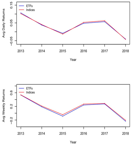
Figure 1. Average Returns. These graphs show the daily (top) and weekly (bottom) average returns of ETFs and indices of our sample per year.

Then, we computed the TEs from Equation (2). Table 3 reports the summary statistics for the annualized tracking errors for both samples. Panel (A) of Table 3 presents the summary statistics for the ETF daily tracking errors. The average annualized tracking error for the daily sample is 0.0332, which ranged from 0.0276 in 2017 to 0.0372 in 2013. Panel (B) presents the summary statistics for the weekly sample. As noted for the returns, the standard deviations of the tracking errors were higher for the daily sample than for the weekly sample. For the weekly sample, the average annualized tracking error is 0.0224, which ranged from 0.0197 in 2017 to 0.0263 in 2013.

Table 3. Tracking errors.

Panel (A): Daily Sample
Year	ETFs	Tracking Errors
		Mean	Median	St.Dev	Min	Max
2013	182	0.0372	0.0169	0.1310	0.0082	1.7593
2014	194	0.0315	0.0163	0.1133	0.0071	1.5697
2015	203	0.0323	0.0184	0.0514	0.0062	0.6072
2016	219	0.0353	0.0168	0.0495	0.0065	0.4108
2017	237	0.0276	0.0146	0.0346	0.0056	0.2392
2018	249	0.0360	0.0162	0.0437	0.0065	0.3097
Overall	1284	0.0332	0.0165	0.0761	0.0056	1.7593
Panel (B): Weekly Sample
Year	ETFs	Tracking Errors
		Mean	Median	St.Dev	Min	Max
2013	182	0.0263	0.0122	0.1443	0.0051	1.9550
2014	194	0.0199	0.0093	0.1105	0.0021	1.5446
2015	203	0.0207	0.0118	0.0456	0.0029	0.6188
2016	219	0.0239	0.0122	0.0401	0.0032	0.3966
2017	237	0.0197	0.0105	0.0292	0.0028	0.2324
2018	249	0.0241	0.0119	0.0346	0.0027	0.2460
Overall	1284	0.0224	0.0113	0.0760	0.0021	1.9550

The tracking errors are annualized. This table reports the yearly summary statistics of ETF TEs. We followed the method of Cremers and Petajisto (2009) to calculate the TEs. The TEs are derived from Equations (1) and (2).

3.2.2. Principal Component Analysis (PCA)

After computing the TEs in the previous section, we aim to determine whether TEs could accurately capture the risk exposure of ETFs relative to their benchmarks. Crucially, we want to test how consistent TE changes are at different levels of ETF risk exposure. We use Principal Component Analysis (PCA) to extract the underlying risk premiums. PCA is the most widely used method for dimensionality reduction (Pukthuanthong et al., 2018; Kozak et al., 2018; Lee et al., 2014). In this study, we extract the underlying risk factors from the indices (benchmarks) and then use risk premiums from the returns on these indices as explanatory variables for ETFs and index returns. We use the R² from these regressions as indicators of the degree of risk exposure for ETFs and their indices over a period of one year.

The cross-sectional risk factor methodology is applied in five steps:

• For each year, we select the indices with the maximum number of observations. Then, we form a matrix of index returns, R_t, with dimensions R_t = [n × #Ind], where n is the number of observations and Ind is the number of indices for that year.
• We extract the first 10 PCAs from the matrix of index returns and store them in a matrix V_t with dimensions V_t = [#Ind × #Components].
• We multiply the matrix of index returns, R_t, by the PCA components matrix, V_t, to obtain the risk factor loadings matrix RL_t = [R × V].
• We regress each ETF and index return on the 10 factors from RL_t, as follows:

  $${\mathrm{R}}_{{\mathrm{E}\mathrm{T}\mathrm{F}}_{\mathrm{i},\mathrm{t}}}=\mathsf{\alpha }+{\mathsf{\beta }}_1\mathrm{P}\mathrm{C}{\mathrm{A}}_1+{\mathsf{\beta }}_2\mathrm{P}\mathrm{C}{\mathrm{A}}_2+{\dots +\mathsf{\beta }}_{10}\mathrm{P}\mathrm{C}{\mathrm{A}}_{10}+{\mathsf{\epsilon }}_{\mathrm{E}\mathrm{T}{\mathrm{F}}_{\mathrm{i},\mathrm{t}}}$$

  (5)

  $${\mathrm{R}}_{{\mathrm{I}\mathrm{n}\mathrm{d}\mathrm{e}\mathrm{x}}_{\mathrm{i},\mathrm{t}}}=\mathsf{\alpha }+{\mathsf{\beta }}_1\mathrm{P}\mathrm{C}{\mathrm{A}}_1+{\mathsf{\beta }}_2\mathrm{P}\mathrm{C}{\mathrm{A}}_2+{\dots +\mathsf{\beta }}_{10}\mathrm{P}\mathrm{C}{\mathrm{A}}_{10}+{\mathsf{\epsilon }}_{\mathrm{I}\mathrm{n}\mathrm{d}\mathrm{e}{\mathrm{x}}_{\mathrm{i},\mathrm{t}}}$$

  (6)
• We record the R² from each regression for each ETF and index each year.

The R² represents how much of the ETF/index return variations are explained by the variation in the overall index returns. In other words, it represents the underlying risk exposure of ETFs and indices based on the systemic variations in index returns. We apply this methodology to both samples (daily and weekly). We report the summary statistics from the risk analysis in Table 4.

Table 4. Summary statistics of R².

Panel (A): Daily Sample
	R2s for ETFs					R2s for Indices
Year	Mean	Median	St.Dev	Min	Max	Mean	Median	St.Dev	Min	Max
2013	89.083	92.753	12.198	3.610	98.860	93.152	96.008	8.265	41.149	99.844
2014	89.624	93.877	13.135	4.130	99.321	92.873	96.312	10.101	18.307	99.851
2015	90.091	94.679	14.589	7.179	99.382	93.802	97.008	9.087	32.091	99.887
2016	88.173	94.845	18.174	3.055	99.269	93.478	96.635	7.939	52.826	99.855
2017	80.954	89.281	21.974	2.718	98.989	88.313	92.466	12.836	16.989	99.626
2018	85.409	93.941	21.032	4.897	99.495	92.494	96.376	10.946	19.994	99.819
Panel (B): Weekly Sample
	R2s for ETFs					R2s for Indices
Year	Mean	Median	St.Dev	Min	Max	Mean	Median	St.Dev	Min	Max
2013	93.984	96.241	8.459	16.437	99.553	95.419	96.955	5.277	59.948	99.943
2014	94.335	97.261	9.405	22.670	99.794	95.099	96.988	7.149	34.498	99.938
2015	92.872	96.107	10.263	16.067	99.273	94.732	96.987	6.985	54.171	99.897
2016	93.455	97.014	11.012	22.726	99.541	95.891	97.875	5.044	67.315	99.860
2017	87.858	93.278	15.336	13.133	99.153	91.369	94.779	10.137	27.042	99.838
2018	92.527	97.082	12.653	28.117	99.818	95.554	97.889	6.450	40.535	99.921

R²s in % format. The R²s for ETFs are the average R²s of all ETFs in each year. The R²s were derived from cross-sectional regression using Equations (5) and (6).

Table 4 presents the average R²s for the ETFs and indices derived from Equations (5) and (6). Panel (A) reports the results for the daily sample, and Panel (B) reports the results for the weekly sample. For the daily sample, the average R² for ETFs ranges from 80.954% in 2017 to 90.091% in 2015. For the indices, it ranges from 88.313% in 2017 to 93.802% in 2015. For the weekly sample, the average R² for ETFs ranges from 87.858% in 2017 to 94.335% in 2014; for the indices, it ranges from 91.369% in 2017 to 95.891% in 2016.

Table 4 shows that the daily R²s for the ETFs and indices tend to be noisier than the weekly data. Additionally, it demonstrates that a significant portion of variations in ETFs and indices can be explained cross-sectionally by the systemic risk of indices in each particular year. Table 4 indicates that the 10 PCA risk loadings explain the variation in ETFs and index returns very well (with medians around 97%). Therefore, substantial variations in both samples are explained by the systemic variations in indices within a particular year. We believe that the choice of 10 PCA factors is sufficient based on the findings in Table 4. It is important to mention that our focus is on the difference between each ETFs’ R² and the R² of its underlying index. However, since we obtained high R² values, we have a lower chance of other possible explanatory risk factors.

4. Tracking Errors and ETFs Risk Exposure

In this section, we investigate whether tracking errors can capture the risk exposure difference between ETFs and their underlying indices. For each year, we calculated the R² differences as follows:

$${\mathrm{R}}_{{\mathrm{D}\mathrm{i}\mathrm{f}\mathrm{f}\mathrm{e}\mathrm{r}\mathrm{e}\mathrm{n}\mathrm{c}\mathrm{e}}_{\mathrm{i},\mathrm{t}}}^2={\mathrm{R}}_{{\mathrm{E}\mathrm{T}\mathrm{F}}_{\mathrm{i},\mathrm{t}}}^2-{\mathrm{R}}_{{\mathrm{I}\mathrm{n}\mathrm{d}\mathrm{e}\mathrm{x}}_{\mathrm{i},\mathrm{t}}}^2$$

(7)

$${\mathrm{A}\mathrm{b}\mathrm{s}\mathrm{R}}_{{\mathrm{D}\mathrm{i}\mathrm{f}\mathrm{f}\mathrm{e}\mathrm{r}\mathrm{e}\mathrm{n}\mathrm{c}\mathrm{e}}_{\mathrm{i},\mathrm{t}}}^2={|\mathrm{R}}_{{\mathrm{E}\mathrm{T}\mathrm{F}}_{\mathrm{i},\mathrm{t}}}^2-{\mathrm{R}}_{{\mathrm{I}\mathrm{n}\mathrm{d}\mathrm{e}\mathrm{x}}_{\mathrm{i},\mathrm{t}}}^2|$$

(8)

where ${\mathrm{R}}_{{\mathrm{E}\mathrm{T}\mathrm{F}}_{\mathrm{i},\mathrm{t}}}^2$ is the R² from Equation (5) for ETF (i) in year (t), and ${\mathrm{R}}_{{\mathrm{I}\mathrm{n}\mathrm{d}\mathrm{e}\mathrm{x}}_{\mathrm{i},\mathrm{t}}}^2$ is the R² from Equation (6) for index (i) in year (t). Therefore, the ${\mathrm{R}}_{{\mathrm{D}\mathrm{i}\mathrm{f}\mathrm{f}\mathrm{e}\mathrm{r}\mathrm{e}\mathrm{n}\mathrm{c}\mathrm{e}}_{\mathrm{i},\mathrm{t}}}^2$ shows the R² difference between an ETF and its underlying index. A difference in R² of zero indicates that the ETF and its underlying index are exposed to the same risk factors. As the R² difference increases, it implies greater divergence in risk exposures between the ETF and its benchmark index. In our analysis, we examine both the directional difference (Equation (7)) and the absolute difference (Equation (8)). We focus on examining whether ETFs bear risks differently than the indices they mimic. Section 3 presents the results of the PCA and ETF tracking errors. For each year, we sort the ETFs based on the magnitude of their TEs, and we report the difference and absolute difference in R²s, as calculated using Equations (7) and (8), respectively. The following graphs show the relationship between risk exposure and TEs.

Figure 2, Figure 3, Figure 4, Figure 5, Figure 6 and Figure 7 present two graphs each. The x-axes of all graphs represent the ETFs for the year, sorted by the highest TE (from left to right). Each point on the x-axis represents a particular ETF from the sample. The y-axis on the bottom graph represents the ETF’s mean tracking error for each year. The y-axis on the top graph represents the absolute R² difference for each ETF from Equation (8). All the figures reported are based on the weekly sample to minimize noise from the daily sample.

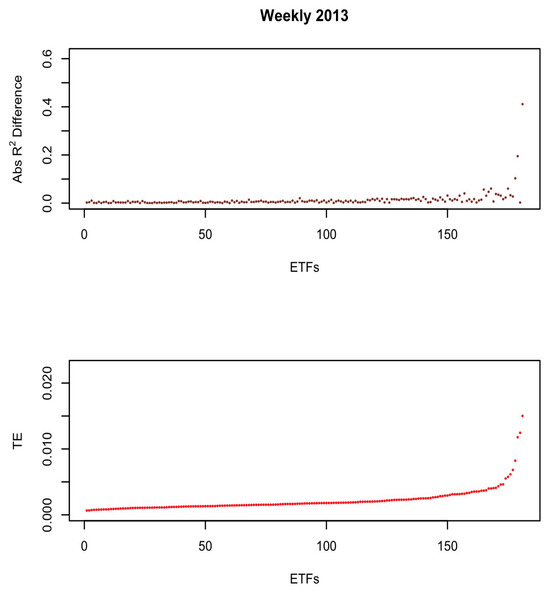
Figure 2. Weekly sample 2013.

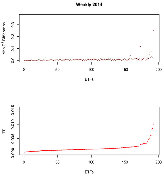
Figure 3. Weekly sample 2014.

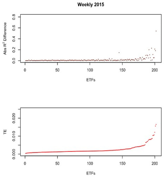
Figure 4. Weekly sample 2015.

Figure 5. Weekly sample 2016.

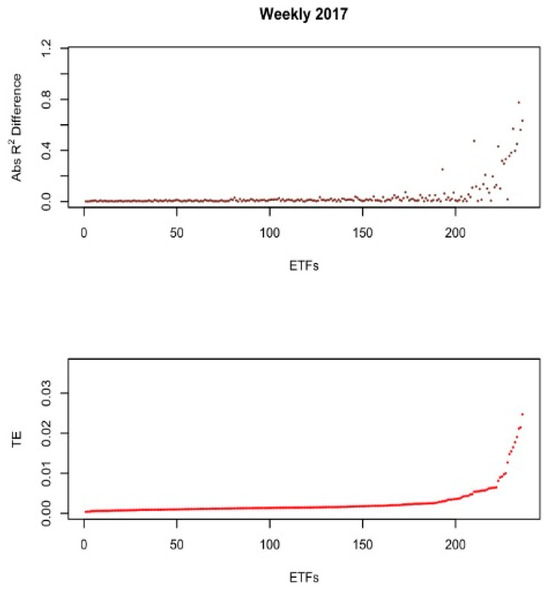
Figure 6. Weekly sample 2017.

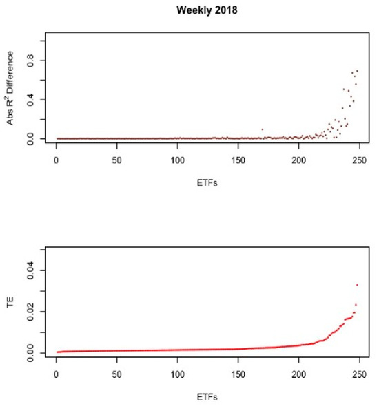
Figure 7. Weekly sample 2018.

Figure 2 shows the relationship between risk exposure and TE for the weekly sample in 2013. It shows that ETFs with the highest tracking errors experience higher variations (gaps) in absolute R² differences. Hence, there are different risk exposures between ETFs and their benchmarks. Importantly, even ETFs with similar TEs can be exposed to different risk levels. These variations are apparent in all years.

Figure 5 shows that some ETFs experience similar risk exposure despite having different levels of TEs. In contrast, Figure 6 shows the absolute R² differences are widely scattered among ETFs with the highest TEs.

These patterns raise questions about how TEs respond to changes in the risk exposure of an ETF and its benchmark, which could be misleading when comparing TEs across ETFs.

To illustrate the variability in risk exposure of ETFs relative to their benchmarks, Table 5 reports the results of Equations (7) and (8) for the daily and weekly samples. For the weekly sample, we find that the AbsR² difference, on average, ranges from 0.820% in 2014 to 3.687% in 2017, indicating higher variations from one year to the next.

Table 5. R² and absolute R² differences.

Panel (A): Daily Sample
	R2 Differences					Absolute R2 Differences
Year	Mean	Median	St.Dev	Min	Max	Mean	Median	St.Dev	Min	Max
2013	−3.995	−1.589	6.582	−51.763	3.781	4.099	1.687	6.517	0.053	51.763
2014	−3.231	−1.166	6.872	−53.585	10.092	3.408	1.248	6.786	0.090	53.585
2015	−3.633	−1.010	9.626	−80.365	6.910	3.807	1.079	9.558	0.003	80.365
2016	−4.955	−0.955	15.010	−86.884	23.143	5.445	1.022	14.838	0.018	86.884
2017	−6.973	−1.885	16.375	−89.288	36.001	7.337	1.923	16.215	0.053	89.288
2018	−6.169	−0.808	16.687	−90.131	57.699	6.771	0.856	16.452	0.007	90.131
Panel (B): Weekly Sample
	R2 Differences					Absolute R2 Differences
Year	Mean	Median	St.Dev	Min	Max	Mean	Median	St.Dev	Min	Max
2013	−1.254	−0.596	3.545	−41.121	1.599	1.351	0.621	3.509	0.008	41.121
2014	−0.732	−0.348	2.166	−24.897	2.064	0.820	0.374	2.134	0.004	24.897
2015	−1.760	−0.601	5.113	−54.230	3.911	1.977	0.673	5.032	0.011	54.230
2016	−2.024	−0.535	7.482	−57.915	9.346	2.236	0.642	7.421	0.002	57.915
2017	−3.126	−0.853	9.424	−56.899	43.110	3.687	0.933	9.218	0.006	56.899
2018	−2.240	−0.222	7.875	−55.810	20.468	2.488	0.291	7.799	0.000	55.810

R²s and Abs R²s differences in % format. This table presents the summary statistics for the R² and absolute R² differences for the daily and weekly samples. The R² differences were calculated using Equation (7), and the absolute R² differences were calculated using Equation (8). The results represent the yearly averages from the weekly and daily samples.

To determine a possible range for the Abs R² difference, we ran 10,000 bootstrap simulations of Equations (5) and (6) for each ETF and index. Then, we calculated the Abs R² differences using Equations (7) and (8). Figure 8 presents the results.

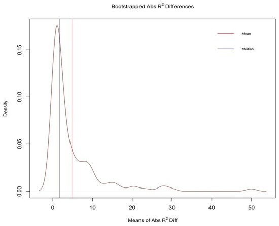
Figure 8. Bootstrapped absolute R² differences.

From the simulations, we find that the absolute R² differences have a mean of 4.808%, a median of 1.702%, and a standard deviation of 7.254. In Section 4.2, we test the impact of changes in absolute R² differences on ETFs’ returns relative to their indices. To further investigate the relationship between R² differences and the level of TE, we rank the TEs each year and report the third and fourth quartiles of TEs and absolute R²s each year. We report the results in Table 6.

Table 6. R² and absolute R² differences by quartiles.

Panel (A): Daily Sample
Year	Quartile	Tracking Errors *	Mean of Absolute R2 Difference
2013	75% to 99% 50% to 75%	0.1744 0.0138	46.732% 3.334%
2014	75% to 99% 50% to 75%	0.1503 0.0100	50.527% 1.792%
2015	75% to 99% 50% to 75%	0.1458 0.0132	56.345% 1.426%
2016	75% to 99% 50% to 75%	0.1726 0.0153	84.233% 1.561%
2017	75% to 99% 50% to 75%	0.1314 0.0100	83.431% 2.727%
2018	75% to 99% 50% to 75%	0.1483 0.0242	86.367% 2.881%
Panel (B): Weekly Sample
Year	Quartile	Tracking Errors *	Mean of Absolute R2 Difference
2013	75% to 99% 50% to 75%	0.0909 0.0049	39.732% 0.768%
2014	75% to 99% 50% to 75%	0.0611 0.0036	24.207% 0.314%
2015	75% to 99% 50% to 75%	0.0934 0.0071	21.517% 0.689%
2016	75% to 99% 50% to 75%	0.1417 0.0083	56.588% 0.677%
2017	75% to 99% 50% to 75%	0.1376 0.0067	61.464% 0.943%
2018	75% to 99% 50% to 75%	0.1462 0.0099	66.416% 0.678%

* Annualized tracking errors.

Panel (A) of Table 6 shows that in 2013, the TE value in the third quartile is 0.0138, while it is 0.1744 in the fourth, representing an increase of 1164%. Meanwhile, the absolute R² increases by about 1302%. In the other years of the sample, the differences between the third and fourth quartiles of TEs and absolute R²s are even greater. For the weekly sample, on average, TEs increases from the third to the fourth quartile by about 1584%, while the absolute R²s increases by about 6680% per year. This indicates that wide risk exposure can occur even for more minor increases in TEs. Therefore, it is fair to argue that TEs may not capture the difference in risk exposure between ETFs and their underlying indices in a consistent and linear manner. This raises the question of whether the difference in absolute R² between an ETF and its benchmark is economically significant. We address this issue in Section 4.2.

4.1. Tracking Errors and the Risk Differences

To further investigate the relationship between TEs and differences in underlying risk factors, we collect ETFs that had complete daily observations from the beginning of 2011 to the end of 2018. We extend our sample to improve the statistical power of the analysis and ensure more reliable estimates. Then, we calculate the monthly TEs for each ETF from Equation (2).

Additionally, we perform PCA for each month and record the absolute R² difference from Equation (8) for each ETF. Following the methods of Madhavan (2016) and Chiu et al. (2012), we also include control variables that affect ETF TEs. The control variables are Premiums, Turnover, Spread, the daily returns on the S&P500 (SPXRet), and VIX. These variables are defined in Appendix A. We use three models derived from the following equation:

$${\mathrm{T}\mathrm{E}}_{\mathrm{i},\mathrm{t}}={\mathsf{\alpha }+{\mathsf{\beta }}_1\mathrm{A}\mathrm{b}\mathrm{s}\mathrm{R}}_{\mathrm{i},\mathrm{t}}^2+{\mathsf{\beta }}_2\mathrm{P}\mathrm{r}\mathrm{e}\mathrm{m}\mathrm{i}\mathrm{u}\mathrm{m}{\mathrm{s}}_{\mathrm{i},\mathrm{t}}+{\mathsf{\beta }}_3{\mathrm{T}\mathrm{u}\mathrm{r}\mathrm{n}\mathrm{o}\mathrm{v}\mathrm{e}\mathrm{r}}_{\mathrm{i},\mathrm{t}}+{\mathsf{\beta }}_4{\mathrm{S}\mathrm{p}\mathrm{r}\mathrm{e}\mathrm{a}\mathrm{d}}_{\mathrm{i},\mathrm{t}}+{\mathsf{\beta }}_5\mathrm{S}\mathrm{P}\mathrm{X}\mathrm{R}\mathrm{e}{\mathrm{t}}_{\mathrm{t}}+{\mathsf{\beta }}_6\mathrm{V}\mathrm{I}{\mathrm{X}}_{\mathrm{t}}+{\mathsf{\epsilon }}_{\mathrm{i},\mathrm{t}}$$

(9)

Table 7 shows a significant and positive relation between TEs and the absolute R² difference in the basic form of Equation (9). Specifically, the TE changes by about 0.01793 for every 0.01 increase in the absolute R² difference. The absolute R² coefficient remains significant and positive when we add the control variables (Model 2) and when we add a monthly dummy variable (Model 3). The relationship is highly significant at 1% in the three models. The absolute R² differences’ coefficients ranges from 0.01353 to 0.01793. This finding is in line with the results presented in Figure 2, Figure 3, Figure 4, Figure 5, Figure 6 and Figure 7: for smaller increases in TE, the risk exposure differs significantly. Additionally, this finding suggests that one should exercise caution when comparing TEs across ETFs to make investment decisions. Consistent with the literature, ETF premiums, turnover, SPX returns, and VIX have a significant impact on TEs. The number of observations is different between Model 1 and Models 2 and 3 due to missing data for the Premiums variable. Model 1 results are robust even when using the same sample as for Models 2 and 3.

Table 7. Panel regression.

	Model 1	Model 2	Model 3
	TE	TE	TE
Abs R2Diff	0.01793 *** (47.88)	0.01371 *** (35.71)	0.01353 *** (35.11)
Premiums		0.00040 *** (3.99)	0.00042 *** (4.18)
Turnover		0.00237 *** (4.09)	0.00239 *** (4.13)
Spread		5.31 × 10−8 (0.17)	−2.56 × 10−9 (−0.01)
SPX Ret		0.00155 ** (3.02)	0.00156 ** (3.04)
VIX		0.00005 *** (11.59)	0.00005 *** (11.93)
Month FE			0.00002 *** (4.63)
Constant	0.00119 *** (72.51)	0.00024 *** (3.64)	0.00011 (1.59)
Obs.	12,000	7594	7594
R2	0.1618	0.1623	0.1647
ETFs	125	125	125

This table reports the results for the three models derived from Equation (9). T-statistics in parentheses. * p < 0.05, ** p < 0.01, *** p < 0.001.

4.2. Economic Significance

A pertinent question at this point is: what is the economic impact of changes in the R² differences between ETFs and their underlying indices? We address this question in Table 8.

Table 8. Economic significance.

Year	Average Changes in Return Difference
2012	−0.0513% **
2013	0.0085%
2014	−0.0742% *
2015	0.0035%
2016	0.0597%
2017	−0.0139% *
2018	0.0034%
2012–2018	−0.0166% **

This table reports the economic impact of changes in the AbsR² difference (Equation (8)) on the average absolute monthly return difference between ETFs and their indices. * p < 0.1; ** p < 0.05; *** p < 0.01.

Table 8 presents the absolute return difference (average per month) between ETFs and their indices when the absolute R² difference (as defined in Equation (8)) changes by 100 basis points. Over the period from 2012 to 2018, we find that a 100-basis-point change in absolute R² difference impacts the return difference by approximately 0.0166% per month on average. Therefore, given the monthly returns (Table 2), we argue that the change in absolute R² is not only impactful regarding risk but also regarding returns.

Our study offers insights into the importance of recognizing the real risk exposure that investors face when they hold an index ETF, which is hard to judge based on the TE alone. Minor changes in the levels of TE can expose investors to risk factors that exceed the exposure of the benchmarks. This differentiation is important for investors, as their investment goals could be heavily compromised.

5. Conclusions

As passive investing continues to expand, ETFs now account for a substantial share of managed assets, and TE is considered a central metric used by investors, regulators, and asset managers to assess fund tracking quality. Our results suggest that reliance on TE alone may be problematic. If the TE does not accurately reflect differences in underlying risk exposure, this may heavily impact investors’ ability to achieve their investment goals.

Motivated by this concern, we examine the usefulness of TE as a measure of risk when making investment decisions. We use the standard PCA approach to assess the underlying risk factors of ETFs and their benchmarks. This framework allows us to evaluate ETF risk exposure directly, rather than inferring it from TE. We find that cross-sectional variation in ETF returns is largely explained by systematic variation in index risk factors. Importantly, even modest differences in TE are associated with economically meaningful divergences in underlying risk exposure relative to the benchmark. These findings imply that comparing TEs across index ETFs may be misleading for investors seeking benchmark-consistent risk exposure. Rather than reflecting a deliberate risk–return tradeoff, TE in ETFs can mask substantial differences in factor exposure, potentially exposing investors to risks for which they are not adequately compensated. Our results have implications for both academic research and practice. For investors, they highlight the limitations of tracking error as a standalone performance metric. For regulators and market participants, they underscore the importance of transparency regarding index replication and underlying risk exposure. Future research could extend our analysis to non-U.S. markets, alternative asset classes, or different ETF replication strategies to further assess the generalizability of these findings.

References

- Aber, J. W., Li, D., & Can, L. (2009). Price volatility and tracking ability of ETFs. Journal of Asset Management, 10, 210–221. [Google Scholar] [CrossRef]
- Ang, A. (2014). Asset management: A systematic approach to factor investing. Oxford University Press. [Google Scholar]
- Bae, K., & Kim, D. (2020). Liquidity risk and exchange-traded fund returns, variances, and tracking errors. Journal of Financial Economics, 138(1), 222–253. [Google Scholar] [CrossRef]
- Carhart, M. M. (1997). On persistence in mutual fund performance. The Journal of Finance, 52, 57–82. [Google Scholar] [CrossRef]
- Chen, N.-F., Roll, R., & Ross, S. A. (1986). Economic forces and the stock market. Journal of Business, 59, 383–403. [Google Scholar] [CrossRef]
- Chiu, J., Chung, H., Ho, K. Y., & Wang, G. H. (2012). Funding liquidity and equity liquidity in the subprime crisis period: Evidence from the ETF market. Journal of Banking & Finance, 36(9), 2660–2671. [Google Scholar] [CrossRef]
- Chu, P. K. K. (2011). Study on the tracking errors and their determinants: Evidence from Hong Kong exchange traded funds. Applied Financial Economics, 21(5), 309–315. [Google Scholar] [CrossRef]
- Cremers, K. M., & Petajisto, A. (2009). How active is your fund manager? A new measure that predicts performance. The Review of Financial Studies, 22, 3329–3365. [Google Scholar] [CrossRef]
- Dorocáková, M. (2017). Comparison of ETF’s performance related to the tracking error. Journal of International Studies, 10(4), 154–165. [Google Scholar] [CrossRef]
- Fama, E. F., & French, K. R. (2015). Incremental variables and the investment opportunity set. Journal of Financial Economics, 117, 470–488. [Google Scholar] [CrossRef]
- Fraś, A., & Rogowski, W. (2016). The attractiveness of passive forms of investment in Poland. Journal of Management and Financial Sciences, 9(25), 43–60. [Google Scholar]
- Frino, A., & Gallagher, D. R. (2001). Tracking S&P 500 index funds. The Journal of Portfolio Management, 28, 44–55. [Google Scholar] [CrossRef]
- Grinold, R., & Kahn, R. (1999). Active portfolio management: A quantitative approach for providing superior returns and controlling risk. McGraw-Hill Professional. [Google Scholar]
- Hougan, M. (2015). Tracking difference, the perfect ETF metric. ETF.com. Available online: https://www.etf.com/sections/blog/tracking-difference-perfect-etf-metric?nopaging=1 (accessed on 23 August 2025).
- Kim, J., Cho, H., & Seok, S. (2023). Liquidity risk, return performance, and tracking error: Synthetic vs. physical ETFs. Journal of International Financial Markets, Institutions and Money, 89, 101885. [Google Scholar] [CrossRef]
- Kostovetsky, L. (2003). Index mutual funds and exchange-traded funds. The Journal of Portfolio Management, 29, 80–92. [Google Scholar] [CrossRef]
- Kozak, S., Nagel, S., & Santosh, S. (2018). Interpreting factor models. The Journal of Finance, 73, 1183–1223. [Google Scholar] [CrossRef]
- Lee, H. C., Tseng, Y. C., & Yang, C. J. (2014). Commonality in liquidity, liquidity distribution, and financial crisis: Evidence from country ETFs. Pacific-Basin Finance Journal, 29, 35–58. [Google Scholar] [CrossRef]
- Lettau, M., & Madhavan, A. (2018). Exchange-traded funds 101 for economists. Journal of Economic Perspectives, 32(1), 135–154. [Google Scholar] [CrossRef]
- Lintner, J. (1965). The valuation of risk assets and the selection of risky investments in stock portfolios and capital budgets. The Review of Economics and Statistics, 47, 13–37. [Google Scholar] [CrossRef]
- Madhavan, A. N. (2016). Exchange-traded funds and the new dynamics of investing. Oxford University Press. [Google Scholar]
- Mossin, J. (1966). Wages, profits, and the dynamics of growth. The Quarterly Journal of Economics, 80, 376–399. [Google Scholar] [CrossRef]
- Poterba, J. M., & Shoven, J. B. (2002). Exchange-traded funds: A new investment option for taxable investors. American Economic Review, 92, 422–427. [Google Scholar] [CrossRef]
- Pukthuanthong, K., Roll, R., & Subrahmanyam, A. (2018). A protocol for factor identification. The Review of Financial Studies, 32, 1573–1607. [Google Scholar] [CrossRef]
- Roll, R. (1992). Industrial structure and the comparative behavior of international stock market indices. The Journal of Finance, 47(1), 3–41. [Google Scholar] [CrossRef]
- Saunders, K. T. (2018). Analysis of international ETF tracking error in country-specific funds. Atlantic Economic Journal, 46(2), 151–160. [Google Scholar] [CrossRef]
- Sharpe, W. F. (1964). Capital asset prices: A theory of market equilibrium under conditions of risk. The Journal of Finance, 19, 425–442. [Google Scholar] [PubMed]
- Shin, S., & Soydemir, G. (2010). Exchange-traded funds, persistence in tracking errors and information dissemination. Journal of Multinational Financial Management, 20(4–5), 214–234. [Google Scholar] [CrossRef]
- Stambaugh, R. F. (2014). Investment noise and trends. The Journal of Finance, 69(4), 1415–1453. [Google Scholar] [CrossRef]
- Treynor, J. L. (1961). Market value, time, and risk (Working paper). Available online: https://papers.ssrn.com/sol3/papers.cfm?abstract_id=2600356 (accessed on 18 January 2026).
- Tzioumis, K., & Barbopoulos, L. G. (2025). Betas distribution and ETF tracking error. SSRN Electronic Journal. [Google Scholar] [CrossRef]
- Yadav, P. K., & Pope, P. F. (1994). Stock index futures mispricing: Profit opportunities or risk premia? Journal of Banking & Finance, 18(5), 921–953. [Google Scholar] [CrossRef]
Disclaimer/Publisher’s Note: The statements, opinions and data contained in all publications are solely those of the individual author(s) and contributor(s) and not of MDPI and/or the editor(s). MDPI and/or the editor(s) disclaim responsibility for any injury to people or property resulting from any ideas, methods, instructions or products referred to in the content. |
© 2026 by the authors. Licensee MDPI, Basel, Switzerland. This article is an open access article distributed under the terms and conditions of the Creative Commons Attribution (CC BY) license.