Performance and Risk Analytics of Asian Exchange-Traded Funds

Abstract

Exchange-traded funds (ETFs) provide low-cost, liquid access to broad equity and fixed-income exposures, including rapidly growing Asian and Asia-focused markets. Yet the academic evidence on Asian ETF portfolio construction remains fragmented, often limited to narrow country samples and centered on mean–variance trade-offs and standard performance statistics, with comparatively less emphasis on downside tail risk and on implementable long-only versus long–short designs under leverage constraints. This study examines the performance and risk characteristics of 29 Asian and Asia-focused ETFs over 2014–2025 and evaluates whether optimization using variance-based and tail-sensitive risk measures improves portfolio outcomes relative to a simple, implementable benchmark. We construct Markowitz mean–variance and conditional value-at-risk (CVaR) efficient frontiers and implement six optimized portfolios at the 95% and 99% tail levels under long-only and long–short configurations with leverage up to 30%. Performance is evaluated relative to an equally weighted Asian ETF benchmark using the Sharpe ratio and tail-sensitive measures, including the Rachev ratio and the stable tail adjusted return (STARR), complemented by fat-tail diagnostics based on the Hill tail-index estimator. The empirical results show that optimization improves efficiency relative to equal weighting in risk-adjusted terms and that moderate leverage can increase returns but typically amplifies volatility, dispersion, and drawdowns. Taken together, the evidence indicates that risk-measure choice materially affects portfolio composition and realized outcomes, with tail-based optimization generally producing more robust allocations than mean–variance approaches when downside risk is a primary concern.

1. Introduction

Exchange-traded funds (ETFs) are open-end index funds that provide daily transparency of their holdings and trade on exchanges like stocks, offering investors intraday liquidity and real-time pricing. The first ETF was launched in 1990 on the Toronto Stock Exchange to track the TSE-35 index, and early research focused on their structure, tax efficiency, and trading properties (Mittal & Richu, 2017). Over the past quarter century, ETFs have emerged as a highly popular passive investment vehicle due to increasing demand for passive strategies, low transaction costs, and high liquidity, which distinguish them from traditional index funds (Liebi, 2020). By 2016, ETFs accounted for over 10% of U.S. market capitalization and more than 30% of overall trading volume (Ben-David et al., 2016). Structurally, ETFs are pooled investment vehicles that combine features of mutual funds and individual securities: they typically track an index, sector, theme, or rules-based strategy, are traded intraday on exchanges at market prices, and use a creation and redemption mechanism with authorized participants to keep prices close to net asset value. The ETF universe now includes broad market and regional funds, single-country funds, sector and industry funds, factor and smart beta products, commodity and currency ETFs, and fixed-income ETFs, with further variation in replication methods (physical versus synthetic, full versus sampling) and liquidity provision.

Research on ETFs in different markets consistently highlights several key benefits for investors. ETFs typically offer low management fees relative to actively managed funds, a high degree of transparency regarding their underlying holdings, and convenient, low-cost diversification across countries, sectors, and asset classes (Joshi & Dash, 2024). Because a single ETF can provide exposure to a broad index, sector, or region, investors can achieve diversified portfolios without the need to trade a large number of individual securities. ETFs also facilitate access to markets that might otherwise be difficult or expensive to enter directly, such as emerging or frontier markets, and they are widely used by both retail and institutional investors for strategic asset allocation, tactical tilts, hedging, and liquidity management. From a portfolio construction perspective, these characteristics make ETFs attractive building blocks for implementing both traditional passive strategies and more sophisticated rule-based allocation schemes.

At the same time, the literature documents a number of risks associated with ETF investing. Tracking error and deviations between market prices and net asset value can arise from imperfect index replication, transaction costs, and market frictions, particularly in less liquid underlying markets (Bahadar et al., 2020; Petajisto, 2017; Zawadzki, 2020). International and emerging-market ETFs may be exposed to additional sources of risk related to currency movements, capital controls, and limited depth in local markets, which can increase volatility and reduce the effectiveness of arbitrage (Cheng et al., 2008; Hilliard & Le, 2022; Jares & Lavin, 2004). Empirical studies also show that ETF trading can affect price dynamics in the underlying securities, potentially amplifying volatility, contributing to co-movement, and increasing tail dependence and contagion during periods of market stress (Ning et al., 2024). While ETFs are often perceived as low-cost, passive instruments, evidence suggests that they do not always outperform the market once costs, liquidity, and structural frictions are taken into account (Blitz & Vidojevic, 2021). These findings underscore that, although ETFs offer important advantages, their use in portfolio construction requires careful attention to tracking behavior, liquidity conditions, and extreme downside risk.

Since their inception, ETFs have attracted substantial academic attention, resulting in a growing body of literature examining their performance, market dynamics, and international expansion. Research has investigated ETFs in diverse regions, including Japan (Rompotis, 2024a), India (Malhotra & Sinha, 2023), China (Ning et al., 2024; Wu et al., 2021), Russia (Tarassov, 2016), and the Asia–Pacific region more broadly (Marszk et al., 2019; Rompotis, 2024b), highlighting differences in market development, trading efficiency, and risk characteristics. Studies have documented that ETFs in emerging markets often exhibit higher trading costs, lower liquidity, and limited arbitrage efficiency compared to their developed-market counterparts (Cheng et al., 2008; Hilliard & Le, 2022; Jares & Lavin, 2004). Recent work on Pakistan-exposed ETFs further underscores the relevance of frontier markets, revealing that careful risk assessment and portfolio optimization are critical for capturing growth opportunities while managing exposure (Jaffri et al., 2025). Beyond geography, research has examined ETFs across asset classes. Commodity-focused ETFs, and gold ETFs in particular, have been analyzed as liquid, accessible instruments for diversification and risk management, with studies examining their safe-haven properties during periods of market stress and their impact on prices and market stability (Wang et al., 2010; Yeniley, 2025). Systematic reviews show that ETF research has expanded to cover volatility, liquidity, risk–return trade-offs, and emerging themes such as ESG and AI-driven strategies (Joshi & Dash, 2024), demonstrating that ETFs’ global reach and cross-asset presence create both opportunities and challenges for investors.

Despite this growing body of work, several important gaps remain in the literature on Asian and Asia-focused ETFs. First, most existing studies examine a small subset of country-specific funds or focus on single-market case studies, which limits our understanding of how different types of Asian and Asia-focused ETFs—such as broad regional funds, country funds, dividend-oriented and small-cap emerging-market ETFs, sector- and industry-focused funds, and fixed-income ETFs—jointly contribute to regional diversification and risk management. Second, prior research on Asian ETFs typically emphasizes mean–variance trade-offs or basic performance statistics, while paying comparatively less attention to downside risk, tail dependence, and the behavior of ETF portfolios under extreme market conditions. Third, there is limited evidence on how long-only versus long–short strategies, and different levels of leverage, affect the risk–return efficiency and tail risk of Asian ETF portfolios over realistic investment horizons. As a result, investors and researchers lack a unified, empirically grounded framework for comparing risk-adjusted performance, tail-risk exposure, and robustness across a broad cross-section of Asian and Asia-focused ETFs, even though portfolio optimization and risk control are central themes in the ETF literature (Vu & Tskhoidze, 2021; Young & Chuahay, 2019).

To address these gaps, the present study focuses on Asian and Asia-focused ETFs and aims to extend existing research through a comprehensive analysis of 29 ETFs across the region. The dataset includes broad regional and country-specific equity funds, dividend-oriented and small-cap emerging-market ETFs, sector- and industry-focused ETFs, and an emerging-market high-yield bond ETF, allowing us to study both emerging and more developed Asian exposures within a single framework. The risk–return structure is evaluated using Markowitz’s mean–variance framework (Markowitz, 1952), which identifies portfolios that maximize expected return for a given level of variance-based risk, alongside conditional value at risk (CVaR), which captures potential extreme losses. We construct six optimized portfolios—a minimum-variance portfolio, a tangent portfolio, and four CVaR-based portfolios at the 95% and 99% levels—under both long-only and long–short configurations with leverage up to 30%. Portfolio performance is evaluated relative to an equally weighted Asian ETF benchmark using the Sharpe, Rachev, and stable tail adjusted return (STARR) ratios, and we complement these results with fat-tail and tail-index diagnostics.

The main aim of the study is to assess how optimization based on variance and tail-sensitive risk measures changes the risk–return and extreme-loss profiles of Asian ETF portfolios relative to a naive equally weighted allocation. More specifically, we address three research questions: (i) How heterogeneous is tail behavior across different types of Asian and Asia-focused ETFs, and what are the implications for portfolio construction and diversification? (ii) How do Markowitz- and CVaR-based optimized portfolios of Asian and Asia-focused ETFs perform relative to an equally weighted benchmark in terms of risk-adjusted returns? (iii) How do long-only and long–short strategies, at different leverage levels, alter the risk–return trade-off and tail-risk exposure of Asian ETF portfolios? The analysis is guided by modern portfolio theory and empirical evidence on heavy-tailed return distributions.

Our analysis employs time-series price data, efficient frontier estimation, and fat-tail risk assessment to provide a comprehensive view of the opportunities and challenges associated with Asian and Asia-focused ETFs. In doing so, the study extends earlier research on Asian ETF portfolio optimization (Young & Chuahay, 2019) by incorporating a broader ETF universe, multiple risk measures, and explicit leverage and tail-risk considerations. The findings offer both methodological insights for portfolio optimization with heavy-tailed assets and practical guidance for investors seeking robust and well-diversified exposure to Asian and emerging markets.

The remainder of the paper is organized as follows. Section 2.1 describes the Bloomberg dataset, the construction of the equally weighted benchmark portfolio, and the rolling-window design used for out-of-sample evaluation. Section 2.3 presents the tail-risk diagnostics based on the Hill tail-index estimator, which motivates the use of tail-sensitive risk measures in this ETF universe. Section 2.4 develops the portfolio construction framework, including the Markowitz mean-variance and CVaR optimization problems and the long-only versus long–short leverage specifications. Section 2.5 defines the risk-adjusted performance measures used in the empirical evaluation, including the Sharpe, Rachev, and STARR ratios. Section 3 reports the first set of empirical results by documenting benchmark behavior and tail-risk heterogeneity across the ETF universe, including cumulative performance evidence and Hill tail-index comparisons for the EQW portfolio, individual ETFs, and the DJIA reference series. Section 4.1 reports the efficient frontier evidence and Section 4.2 evaluates cumulative wealth paths under long-only and long–short implementations, followed by the ratio-based results in Section 4.3. Section 5 discusses economic interpretation and practical implications, and Section 6 concludes.

2. Materials and Methods

2.1. Data Description

The dataset for this study was obtained from Bloomberg Professional Services and covers the period from 10 December 2014 to 30 January 2025. A total of 29 exchange-traded funds (ETFs) were selected to provide broad coverage of Asian and Asia-focused markets, with the inclusion of a small number of broad emerging-market funds to enable comparison with the wider emerging-market universe. Many of the economies represented in this sample, such as China, India, South Korea, Taiwan, Malaysia, Thailand, Indonesia, the Philippines, and Vietnam, are classified as emerging markets by MSCI and FTSE. Consequently, the ETFs in our dataset capture both Asian regional exposures and emerging-market characteristics, reflecting Asia’s dual role as one of the largest and fastest-growing components of global emerging-market indices.

The sample incorporates a diverse mix of broad regional ETFs, country-specific ETFs, sector-focused ETFs, dividend-oriented funds, small-cap emerging-market ETFs, and a high-yield emerging-market bond ETF. This composition ensures that the dataset reflects both the structural growth opportunities within Asia and the diversification benefits that arise from cross-country and cross-sector allocation. Table A1 in Appendix A presents the complete list of ETFs included in the analysis, along with their Bloomberg tickers, full fund names, and investment focus.

In addition to the ETF universe, we include the Dow Jones Industrial Average (DJIA) as a reference developed-market index representing U.S. large-cap equities. The 3-month and 1-year U.S. Treasury yields, obtained from Bloomberg, are employed as proxies for the risk-free rate over the same period. Historical optimization is performed using a rolling window of approximately four trading years (4 × 252 trading days), which balances the need for sufficient data to estimate return and risk parameters with the desire to keep the estimation window responsive to changing market conditions.

2.2. Benchmark Construction

For benchmarking purposes, we construct an equally weighted portfolio (EQW) of the 29 ETFs. The EQW assumes a 100-dollar long-only investment in each ETF as of 10 December 2014 and is rebalanced daily to maintain equal weights across all funds. By definition (Markowitz, 1952; Sharpe et al., 1999), an EQW is a simple, non-optimized allocation that invests the same proportion of capital in each asset, providing a neutral, diversified baseline against which we can evaluate the gains from optimization.

2.3. Tail-Risk Diagnostics Methodology

Because our analysis places particular emphasis on downside and extreme risk, it is important to first understand the tail properties of the return distributions for the EQW and the 29 individual Asian and Asia-focused ETFs. Tail behavior determines the frequency and severity of extreme returns and therefore has direct implications for risk management, the choice of performance measures, and the suitability of variance-based versus tail-based optimization criteria. We also include the DJIA as a reference developed-market index representing a mature, highly liquid U.S. large-cap market. Comparing the tail behavior of the Asian ETF portfolios to the DJIA serves two purposes: it provides a familiar benchmark for gauging the magnitude of tail risk in economic terms, and it allows us to assess whether reallocating from a standard U.S. equity exposure to Asian and Asia-focused ETFs entails materially heavier tail risk. This is directly related to our first research question, which concerns how heterogeneous tail behavior is across different types of Asian and Asia-focused ETFs and what this implies for portfolio construction and diversification.

Hill Estimator for Tail Index Measurement

To assess tail heaviness, we use the classical Hill estimator (B. M. Hill, 1975), a widely used nonparametric method for estimating the tail index of heavy-tailed distributions. Suppose we have a sample of independent and identically distributed random variables whose distribution satisfies

$$P(X>x)=x^{-\alpha }L\left(x\right),\mathrm{for}x\ge 0,$$

where $L\left(x\right)$ is a slowly varying function and $\alpha >0$ is the tail index, which measures how heavy the tail is. A smaller value of $\alpha$ indicates heavier tails and a higher likelihood of extreme outcomes.

The Hill estimator is commonly expressed as

$${\widehat{\alpha }}^{-1}={\displaystyle \frac{1}{k}}\sum _{i=1}^{k}ln\left({\displaystyle \frac{X_{\left(i\right)}}{X_{(k+1)}}}\right),$$

where $X_{\left(1\right)}\ge X_{\left(2\right)}\ge \dots \ge X_{(k+1)}$ are the largest order statistics of the sample. In simple terms, the Hill estimator measures the average spacing between the largest observations relative to a threshold, providing a quantitative measure of how slowly the tail of the distribution decays. The smaller the estimated $\alpha$, the heavier the tail of the return distribution, meaning that extreme losses or gains occur more frequently.

Over time, several studies have refined and extended Hill’s methodology to address its limitations and enhance robustness in financial applications. For example, Wagner and Marsh (2000) proposed adaptive estimators to handle dependence structures such as ARCH-type processes, while Brilhante et al. (2013) developed a generalized version to correct bias and incorporate higher-order moments. Similarly, Aban and Meerschaert (2001) introduced a shifted version of the estimator to achieve scale and shift invariance, and J. B. Hill (2010) examined its asymptotic properties under dependence and heterogeneity in financial time series. The Hill estimator remains widely used because of its flexibility and diagnostic usefulness in empirical finance. Drees et al. (2000) provided guidance on constructing Hill plots to visualize tail index estimates, while Davletov (2022) demonstrated its practical application in analyzing the heavy-tailed behavior of equity returns, highlighting structural breaks during periods of financial distress such as the 2008 Global Financial Crisis.

2.4. Portfolio Construction Framework

Portfolio optimization is a fundamental tool in investment management, aiming to construct portfolios that balance risk and return while accommodating investor preferences, constraints, and uncertainties. The concept was first formalized by (Markowitz, 1952) through the mean–variance framework, which seeks to maximize expected returns for a given level of risk, where risk is quantified by the portfolio’s return variance. Over time, research has significantly evolved beyond the original mean variance formulation. Salo et al. (2024) provide a comprehensive historical overview of portfolio optimization, highlighting the development of integrated frameworks that address decision makers’ preferences and multiple objectives across planning horizons. Building on this, Liu et al. (2023) introduce dynamic risk preference models and optimization under uncertain environments, applying average value at risk (VaR) frameworks with genetic algorithms to enhance wealth creation and efficiency. Furthermore, comparative analyses such as Sen and Dasgupta (2023) demonstrate that different optimization approaches, ranging from traditional mean variance portfolios to machine learning based designs, yield varying performance outcomes depending on market conditions. Complementing these insights, Ou (2023) emphasize the continued relevance of modern portfolio theory (MPT) in understanding how regulatory, industry specific, and client driven constraints shape portfolio performance.

In Lindquist et al. (2021), both historical and dynamic optimization frameworks are discussed. Historical optimization estimates expected returns and risks using past data, assuming that market relationships remain stable within each estimation window. A rolling-window approach is typically used, providing simplicity and interpretability but limited responsiveness to sudden market shifts or crises. Dynamic optimization, on the other hand, models time-varying behavior in returns and volatility using methods such as ARMA–GARCH processes, fat-tailed (e.g., Student’s t) distributions, and copula-based dependence structures. This approach better captures evolving correlations and tail risks, producing more adaptive portfolios at the cost of higher model complexity and computational demand.

In this paper, we adopt the historical optimization approach. Using daily ETF return data from 2014 to 2025, we use a rolling window where each window spans approximately four years. The optimizer estimates expected returns and covariances for assets within each window and generates portfolio weights for the next trading day. This recursive process produces a continuous series of optimized portfolio weights and returns, reflecting how the strategy would have performed under real historical conditions.

2.4.1. Markowitz Mean–Variance Optimization

Formally, the Markowitz mean–variance optimization problem can be expressed as minimizing portfolio variance subject to a desired expected return and full investment constraint. Let r denote the vector of expected returns, $\Sigma$ the covariance matrix of asset returns, and w the portfolio weights. The optimization problem is given by:

$$\begin{array}{cc}\hfill \underset{w}{min}& w^{\top }\Sigma w\hfill \\ \hfill \mathrm{subject}\mathrm{to}& r^{\top }w={\overline{r}}_p,\hfill \\ & e_n^{\top }w=1,\hfill \end{array}$$

where ${\overline{r}}_p$ is the target portfolio return and $e_n$ is an n-dimensional vector of ones. This problem is solved using the standard Lagrange multiplier method, which introduces auxiliary variables q and ${\theta }_0$ corresponding to the constraints $r^{\top }w={\overline{r}}_p$ and $e_n^{\top }w=1$. The Lagrangian form of the optimization problem is written as:

$$\underset{w,q,{\theta }_0}{min}L(w,q,{\theta }_0)=\underset{w,q,{\theta }_0}{min}\left({\displaystyle \frac{1}{2}}{w}^{\top }\Sigma w+q({\overline{r}}_p-r^{\top }w)+{\theta }_0(1-e_n^{\top }w)\right).$$

Minimizing this Lagrangian with respect to w yields the first-order conditions that define the optimal portfolio weights. The analytical solution can be expressed as:

$$w^{*}={\overline{r}}_p{w}_1+w_2,$$

where

$$w_1={\displaystyle \frac{1}{\Delta }}\left(B{\Sigma }^{-1}r-C{\Sigma }^{-1}{e}_n\right),w_2={\displaystyle \frac{1}{\Delta }}\left(A{\Sigma }^{-1}{e}_n-C{\Sigma }^{-1}r\right).$$

and the scalar constants are defined as

$$A=r^{\top }{\Sigma }^{-1}r,B=e_n^{\top }{\Sigma }^{-1}{e}_n,C=r^{\top }{\Sigma }^{-1}{e}_n,\Delta =AB-C^2.$$

The efficient frontier is then obtained by plotting the portfolio’s standard deviation

$${\sigma }_p=\sqrt{w^{*\top }\Sigma w^{*}}$$

against its expected return ${\overline{r}}_p$, illustrating the trade-off between risk and return. This formulation provides the basis for constructing both the minimum-variance and tangent portfolios in subsequent analyses.

2.4.2. CVaR Optimization

Building on the classical mean–variance framework, we next extend the analysis by incorporating downside tail risk through the CVaR measure, following the approach of Rockafellar and Uryasev (2000) and Krokhmal et al. (2002). While the Markowitz model captures overall variance as a measure of risk, it assumes return distributions are symmetric. In contrast, CVaR focuses specifically on the tail of the loss distribution, measuring the expected loss beyond a specified quantile of returns. This makes it a more suitable framework for managing extreme downside risk, particularly in volatile or asymmetric markets.

Formally, the CVaR optimization problem seeks the portfolio weights w that minimize the expected loss in the worst $\alpha$ proportion of outcomes:

$$\underset{w}{min}{\mathrm{CVaR}}_{\alpha }\left(w\right)\mathrm{subject}\mathrm{to}{r}^{\top }w={\overline{r}}_p,e_n^{\top }w=1.$$

Here, $\alpha$ represents the tail probability (commonly 0.05 or 0.01), corresponding to 95% or 99% confidence levels. The CVaR can be expressed as

$${\mathrm{CVaR}}_{\alpha }\left(w\right)={\mathrm{VaR}}_{\alpha }\left(w\right)+{\displaystyle \frac{1}{\alpha }}\mathbb{E}\left[{(-f(w,r)-{\mathrm{VaR}}_{\alpha }\left(w\right))}^{+}\right],$$

where ${\left(x\right)}^{+}=max(0,x)$ ensures that only returns exceeding the Value-at-Risk threshold contribute to the tail risk. This formulation transforms the problem into a convex optimization, allowing the CVaR frontier to be derived efficiently through linear programming techniques. Compared to the mean–variance frontier, the CVaR frontier explicitly accounts for asymmetry in return distributions and highlights the trade-off between expected return and potential extreme losses, offering a more realistic view of risk exposure under market stress.

2.4.3. Long-Only and Long–Short Strategy Specifications

In this study, we evaluate optimized portfolios under both long-only and long–short investment strategies. The long-only approach restricts all asset weights to non-negative values, representing portfolios that invest exclusively in long positions. In contrast, long–short strategies allow both long and short exposures, enabling investors to profit from assets expected to appreciate while shorting those expected to decline. This flexibility can enhance return potential for a given level of volatility but introduces additional risks, such as margin requirements and potential losses from adverse price movements.

Following the framework of Lindquist et al. (2021), we implement long–short models with leverage levels of 10%, 20%, and 30%, reflecting varying degrees of short position exposure. The Jacobs et al. (1999) model extends the classical mean–variance optimization by allowing the long and short positions to be optimized simultaneously. In their formulation, asset weights are constrained within a range that permits shorting up to a specified proportion of the total portfolio value while maintaining overall balance in the portfolio. The approach assumes daily re-balancing and disregards transaction, margin, or borrowing costs.

Lo and Patel (2008) propose an alternative long–short framework inspired by the 130/30 concept, in which 30% of the capital is obtained through short selling and the proceeds are used to take 130% long positions. Their model includes explicit leverage constraints to control both the extent of short selling and the overall exposure of the portfolio. This approach provides a more structured implementation of leverage while preserving the diversification and efficiency benefits of mean–variance optimization.

The performance of each portfolio is evaluated from December 2018 through January 2025, assuming a USD 100 investment on 11 December 2018. The analysis considers six optimized portfolios: MVP, TVP, M95, T95, M99, and T99, representing both mean–variance and CVaR-based optimization frameworks across different confidence levels. The EQW portfolio serves as a benchmark for comparison.

2.5. Performance Measures

Performance evaluation provides insight into how efficiently a portfolio balances risk and return. While cumulative growth offers an overview of performance, risk-adjusted measures allow for a more robust comparison across portfolios with different risk exposures. In this study we use three complementary ratios, namely the Sharpe ratio, the STARR, and the Rachev ratio, to capture different aspects of portfolio efficiency and tail risk sensitivity. Together, these measures provide a framework for assessing portfolio robustness under both normal and extreme market conditions (Choi et al., 2015; da Fonseca, 2020; Gatfaoui, 2009; Goetzmann et al., 2002; Lo, 2002; Smetters & Zhang, 2013; Steiner, 2011; Zhang, 2025).

2.5.1. Sharpe Ratio

The Sharpe ratio (Sharpe et al., 1999) measures the excess return earned per unit of total risk and is one of the most widely used performance measures in finance. It provides a straightforward way to evaluate the trade-off between risk and return.

There have been several studies on the Sharpe ratio. Lo (2002) highlights that Sharpe ratios can be overstated due to serial correlation and time aggregation effects, meaning that monthly Sharpe ratios cannot simply be annualized by multiplying by $\sqrt{12}$. Goetzmann et al. (2002) demonstrate that Sharpe ratios can be manipulated through option-like payoffs, raising caution when comparing managers who employ derivatives. Gatfaoui (2009) introduces a filtering method to extract “fundamental” Sharpe ratios that are robust to skewness and kurtosis biases, reflecting purer performance indicators. Formally, the Sharpe ratio is defined as

$$SR\left(T\right)={\displaystyle \frac{\mathbb{E}[r_p\left(t\right)-r_f\left(t\right)]}{\sqrt{\mathrm{VAR}[r_p\left(t\right)-r_f\left(t\right)]}}}.$$

(1)

A higher Sharpe ratio indicates greater excess return per unit of volatility. A negative Sharpe ratio occurs when the expected excess return $\mathbb{E}(r_p-r_f)$ is negative, meaning the portfolio under-performs the risk-free rate on average. Because the Sharpe ratio relies on volatility as the risk measure and implicitly favors approximately normal returns, it may not fully capture performance under extreme market conditions.

2.5.2. Rachev Ratio

The Rachev ratio (Rachev et al., 2008) compares average gains in large positive market swings to average losses in large negative swings, making it particularly useful for understanding portfolio behavior under extreme market conditions. It focuses on the asymmetry between the tails of the return distribution rather than overall volatility.

Biglova et al. (2004) introduced this ratio to emphasize the balance between expected tail gains and expected tail losses, and subsequent studies have applied it to stress testing and portfolio construction frameworks. da Fonseca (2020) also includes the Rachev ratio among key performance measures when evaluating international portfolios, finding that it captures reward–risk efficiency better during periods of market stress. The Rachev ratio is defined as

$$R{R}_{\alpha ,\beta }\left(T\right)={\displaystyle \frac{{\mathrm{CVaR}}_{\beta }(r_f\left(t\right)-r_p\left(t\right))}{{\mathrm{CVaR}}_{\alpha }(r_p\left(t\right)-r_f\left(t\right))}},$$

(2)

and is evaluated here at the 95% and 99% confidence levels. Lower values indicate that, in the tails, extreme gains tend to dominate extreme losses.

2.5.3. STARR Ratio

The STARR builds on the Rachev and Sharpe ratios by focusing on reward per unit of expected tail loss. By replacing volatility with CVaR in its denominator, it captures downside sensitivity more effectively and offers a conservative measure of performance (Rachev et al., 2008).

Rachev et al. (2007) introduced the STARR ratio, and subsequent studies have shown that incorporating CVaR can enhance the robustness of portfolio optimization under turbulent market conditions (Sehgal & Mehra, 2021; Zhang, 2025). The STARR ratio is defined as

$$STARR\left(T\right)={\displaystyle \frac{\mathbb{E}[r_p\left(t\right)-r_f\left(t\right)]}{{\mathrm{CVaR}}_{\alpha }[r_p\left(t\right)-r_f\left(t\right)]}},$$

(3)

so that higher values indicate greater excess return per unit of tail loss.

3. Empirical Results I: Data Characteristics and Tail-Risk Diagnostics

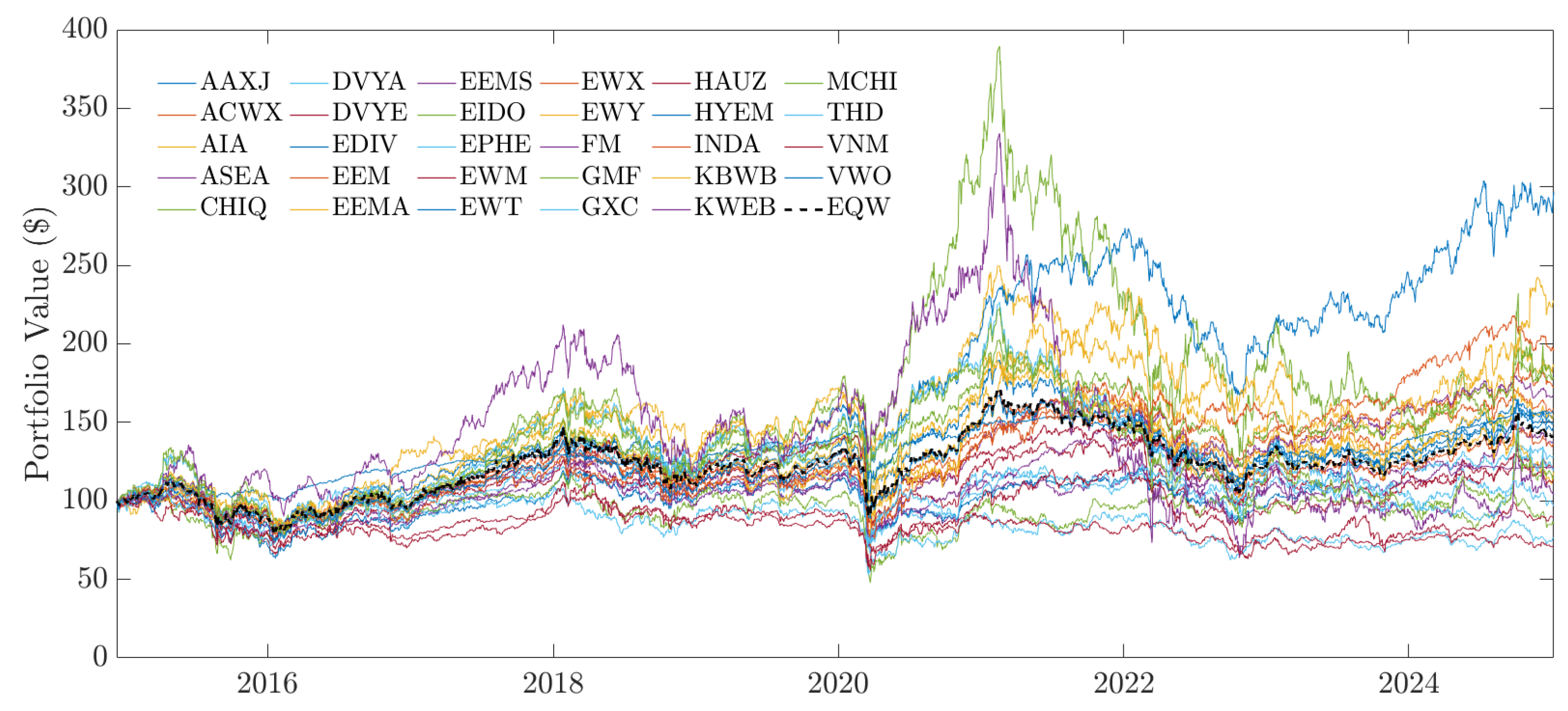
This section reports the empirical evidence that motivates tail-sensitive portfolio construction in this ETF universe. We first describe the benchmark behavior and then summarize the tail-risk diagnostics for the EQW portfolio and individual ETFs, using the Hill estimator methodology outlined in Section 2.3. As shown in Figure 1, the EQW portfolio exhibits greater stability than most individual ETFs in the sample.

Figure 1. Cumulative prices for individual Asian-traded ETFs and EQW, assuming a USD 100 investment on 10 December 2014.

Some country-specific funds such as EWT (Taiwan) and INDA (India) outperform the EQW over the long run, others, including VNM (Vietnam) and HYEM (emerging-markets high-yield bonds), lag behind. The COVID-19 market crash of early 2020 generated a sharp drawdown across all ETFs, but both the EQW and most constituents subsequently recovered, underscoring the resilience of diversified exposure to Asian and emerging markets.

3.1. Benchmark Behavior and Cumulative Performance

This empirical behavior is consistent with prior studies on equal weighting. Jaffri et al. (2025) show that equal weighting enhances diversification and resilience in emerging market-focused ETF portfolios. Malladi and Fabozzi (2017) provide long-term evidence that equally weighted strategies can outperform value-weighted strategies, largely due to systematic re-balancing effects, while Taljaard and Maré (2021) highlight that equal weighting may under-perform in the short run when market concentration rises but tends to remain competitive over longer horizons. Taken together, these findings support our use of the EQW portfolio as the central benchmark: its simplicity, empirical robustness, and consistent performance advantages make it a suitable standard for evaluating the effectiveness of optimized portfolios.

3.2. Empirical Tail Behavior of Asian ETFs, EQW, and DJIA

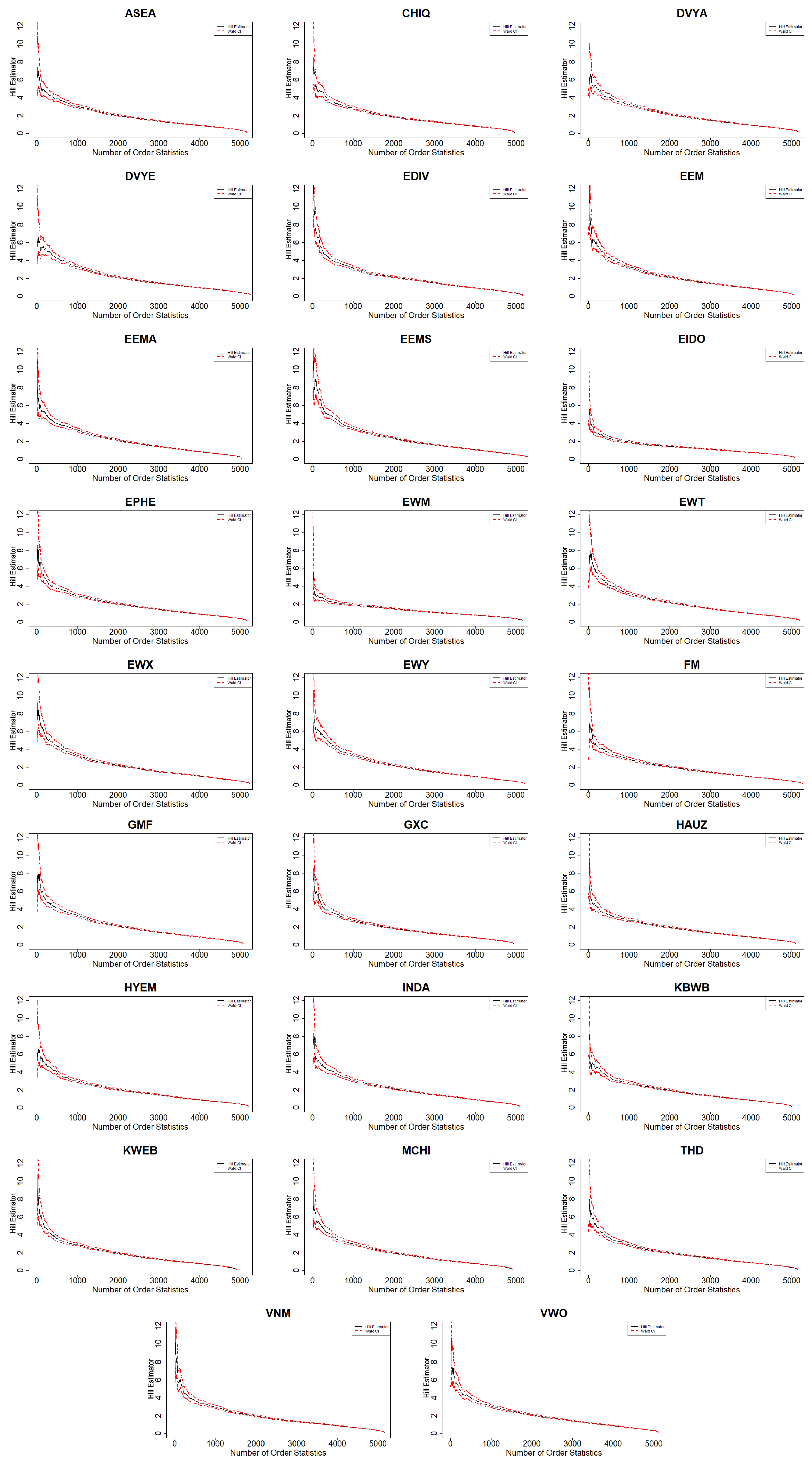
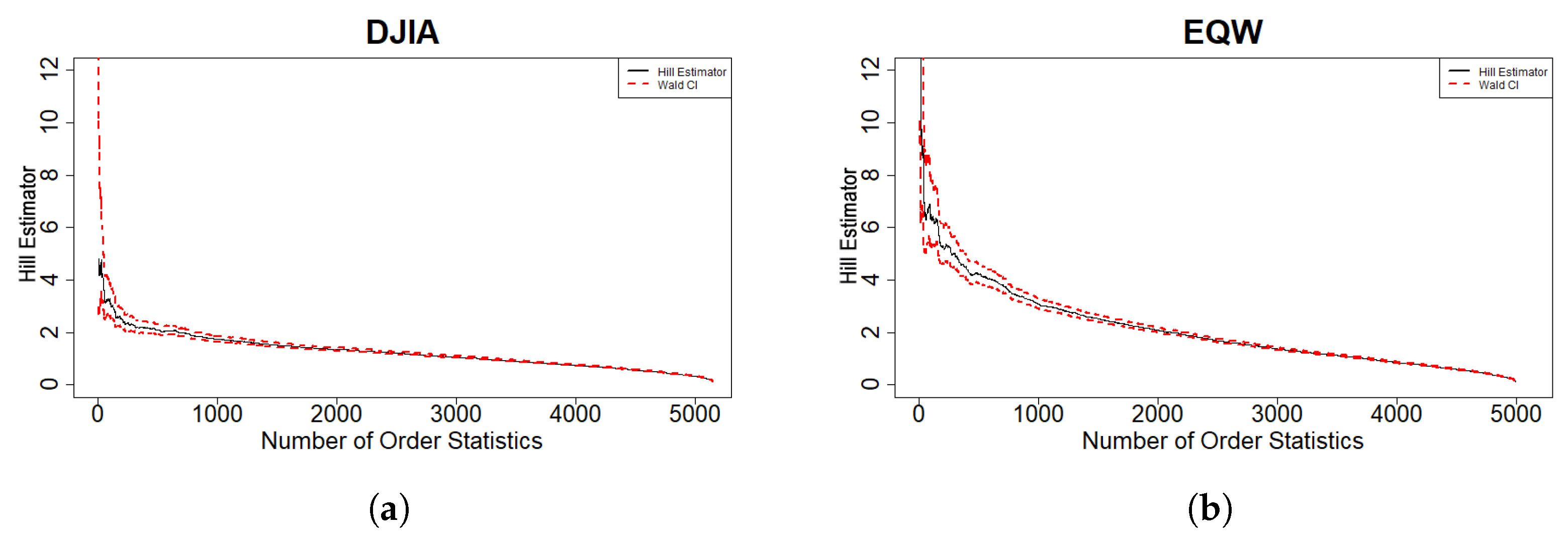
For each return series in our study, we compute the Hill estimator over an increasing number of upper order statistics and plot the resulting Hill curve together with Wald confidence intervals. The initial part of each curve typically shows substantial fluctuation because it is based on only a few extreme observations; as more order statistics are included, the curve tends to stabilize, indicating the range in which the tail index is reasonably estimated. Appendix B reports Hill plots for all 29 ETFs, while Figure 2 compares the DJIA and the EQW portfolio.

Figure 2. DJIA and EQW estimated tail index, along with the Wald confidence interval (CI). (a) DJIA. (b) EQW.

Visual inspection of the DJIA and EQW plots shows that both series exhibit heavy but finite tails, but the nature of that tail risk differs. The Hill curve for the DJIA stabilizes around a higher value of the tail index, suggesting that extreme events decay more rapidly and the likelihood of very large losses is relatively low. In contrast, the EQW portfolio, constructed by allocating equal weights to all 29 Asian and Asia-focused ETFs in our sample, settles at a lower tail-index level and displays wider confidence bands. This indicates that the EQW is more prone to extreme returns and carries greater tail risk than the reference U.S. large-cap index, consistent with the higher volatility and lower liquidity typically associated with emerging and regionally concentrated exposures.

Across the individual ETFs, the Hill curves share a broadly similar shape, but their stabilized levels differ, revealing nontrivial heterogeneity in tail behavior across funds. ETFs with more concentrated, small-cap, or high-yield exposures tend to display somewhat heavier tails, while larger, more diversified regional funds exhibit relatively thinner tails. These differences suggest that extreme risk within the Asian ETF universe is not uniform but depends on the underlying market segment and investment focus.

Taken together, the Hill diagnostics indicate that an equal-weighted allocation to the 29 Asian and Asia-focused ETFs in our sample exhibits heavier tails than the DJIA, and that tail behavior varies meaningfully across ETF types. This motivates the use of tail-sensitive risk measures, such as CVaR and tail-based performance ratios (Rachev and STARR), as complements to mean–variance analysis in the subsequent portfolio optimization and performance evaluation.

4. Empirical Results II: Optimization and Performance Outcomes

This section presents the optimization outcomes and performance evidence generated by the empirical design described in Section 2.4, using the evaluation metrics defined in Section 2.5. For clarity, we report the results in three steps: (i) efficient frontier evidence, (ii) cumulative wealth paths under long-only and long–short implementations, and (iii) risk-adjusted ratio evidence.

We analyze both the Markowitz mean–variance and CVaR optimization frameworks. The CVaR problems are solved at the 95% and 99% confidence levels to examine how increasing tail-risk sensitivity affects portfolio composition and realized performance. We consider six optimized portfolios: the minimum-variance portfolio (MVP) and tangent portfolio (TVP) from the Markowitz frontier, and the minimum-CVaR and tangent-CVaR portfolios at the 95% and 99% levels (M95, T95, M99, and T99). Portfolio performance is assessed relative to the equally weighted benchmark (EQW) under both long-only constraints and long–short strategies with bounded leverage, following Lindquist et al. (2021).

4.1. Markowitz and CVaR Efficient Frontier Results

Figure 3 shows the Markowitz efficient frontiers constructed using the one-year and the three-month Treasury yield as the risk-free rate. Each plot illustrates the trade-off between risk, measured by the standard deviation of portfolio log returns, and expected return, represented by the mean of portfolio log returns. The blue curve traces the efficient frontier, while the red dashed line represents the capital market line that is tangent to the frontier at the optimal, or tangent portfolio. Both graphs exhibit the typical upward-sloping convex shape, indicating that higher returns are associated with higher levels of portfolio risk. The similarity between the two frontiers suggests that the choice between the one-year and three-month Treasury yields has minimal effect on the resulting efficient frontier or the tangent portfolio position.

Figure 3. The Markowitz efficient frontiers using (a) 1-year and (b) 3-month U.S. Treasury yields.

The EQW portfolio lies below the efficient frontier, exhibiting a modestly negative mean return that underscores the efficiency gains from optimization relative to a simple equal-weight allocation. The tangent portfolio, positioned near the upper-left edge of the ETF cluster, sits very close to EDIV, suggesting that this dividend-focused fund performs similarly to the optimal risk-adjusted portfolio. In practical terms, an investor holding EDIV would experience a performance profile that closely mirrors the tangent portfolio, indicating its strong standalone efficiency. Most ETFs cluster tightly around the efficient frontier, showing generally well-balanced risk–return profiles. However, funds such as KWEB deliver higher mean returns at the cost of greater volatility, while CHIQ and MCHI sit below the frontier, reflecting weaker risk-adjusted performance. Overall, the results suggest that diversified and income-oriented exposures dominate the tangent portfolio, reinforcing the advantage of combining stability and moderate growth within the Markowitz framework.

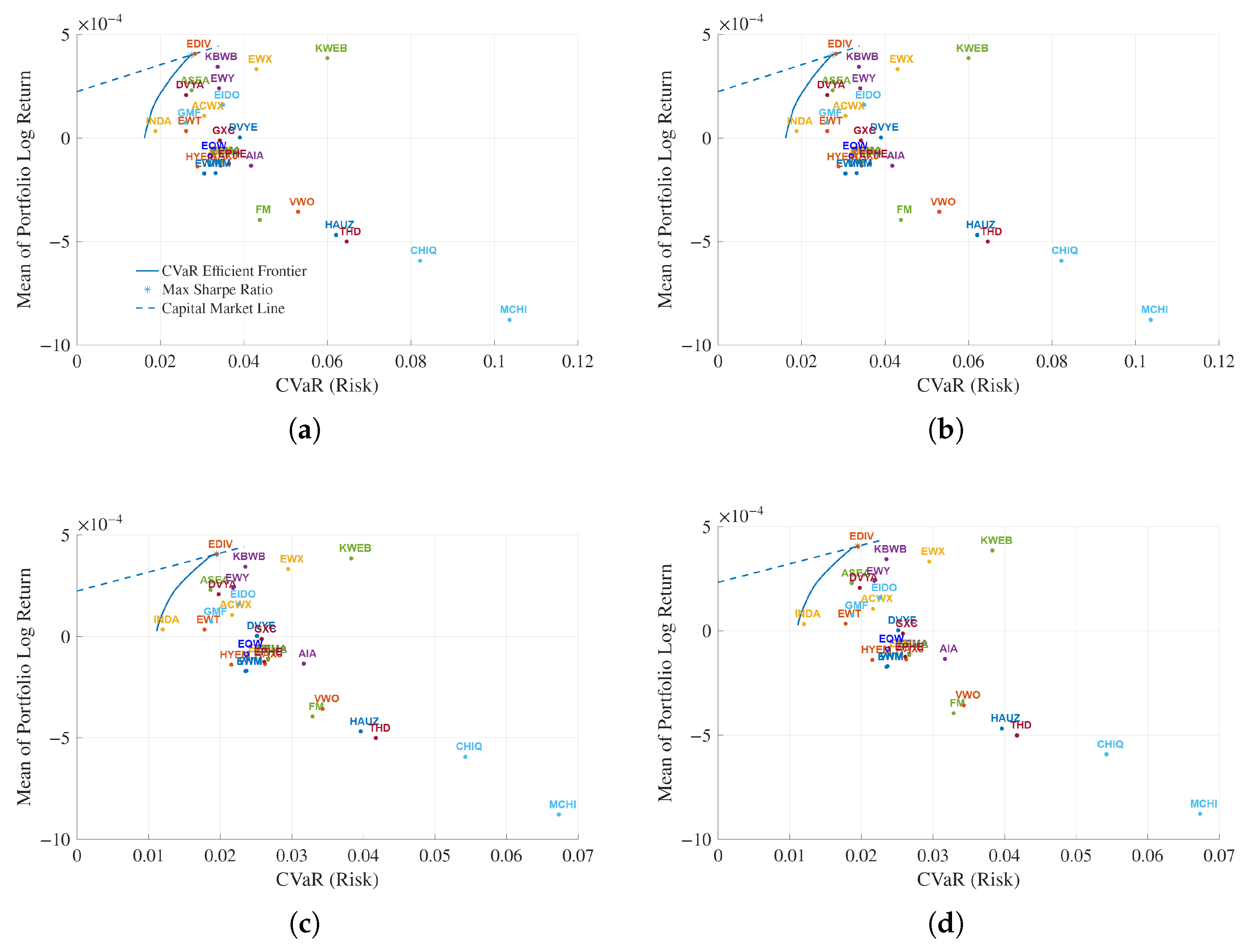
Figure 4 presents the CVaR efficient frontiers at the 99% and 95% confidence levels using both the 1-year and 3-month U.S. Treasury yields as the risk-free rate. Each curve shows the trade-off between expected return and tail-risk exposure, measured by CVaR. As expected, the 99% frontiers exhibit slightly higher CVaR values than the 95%, reflecting the stricter loss quantile that captures rarer and more extreme downside events. This shift confirms that portfolios optimized under higher confidence levels face greater tail-risk for a given expected return, consistent with theory.

Figure 4. CVaR efficient frontiers at the 99% and 95% confidence levels using 1-year and 3-month U.S. Treasury yields as the risk-free rate. The top panels correspond to the 99% level with the 1-year (left) and 3-month (right) yields, while the bottom panels show the 95% level for the same yield horizons. (a) 99% CL, 1-Year. (b) 99% CL, 3-Months. (c) 95% CL, 1-Year. (d) 95% CL, 3-Months.

The maximum Sharpe ratio portfolios, which represent the best trade-off between expected return and tail-risk, remain relatively stable across yield horizons but differ slightly across confidence levels. At the 99% level, the maximum Sharpe ratio portfolio lies close to EDIV, while at the 95% level it aligns almost exactly with EDIV, suggesting that EDIV performs efficiently as a standalone ETF under both risk perspectives. The higher CVaR values observed at the 99% level confirm that portfolios become more sensitive to extreme losses as the confidence threshold tightens. Overall, these results show that CVaR-based optimization preserves the general shape of the Markowitz frontier while emphasizing downside protection and resilience under severe market conditions.

When comparing the individual ETFs to the optimized frontiers, it is clear that most single funds lie below both the Markowitz and CVaR efficient frontiers, indicating lower risk–return efficiency. This suggests that while some ETFs perform reasonably well on their own, diversification across multiple ETFs produces portfolios that achieve higher returns for comparable or lower levels of risk. Lindquist et al. (2021) noted that log returns can generally replace discrete returns in portfolio optimization when daily returns remain small. However, when daily returns become large, typically greater than about 1%, the approximation can introduce significant errors. To confirm that this assumption held for our dataset, we compared the efficient frontiers computed using both log and arithmetic returns. The resulting frontiers were the same, indicating that our data were well within the range where the log-return approximation is valid. Accordingly, the analysis presented here uses log returns throughout.

From an applied perspective, our results suggest that CVaR based optimization is particularly relevant for Asian and Asia-focused ETFs. The Hill tail index diagnostics in Section 3.2 show that the equally weighted Asian ETF portfolio has heavier tails than the DJIA, so extreme losses play a more prominent role in this sample than in a standard U.S. large cap index. In this setting, variance alone may understate downside risk, whereas CVaR directly targets the worst 5% or 1% of outcomes. Within the CVaR framework, the minimum CVaR portfolios (M95 and M99) are designed to reduce exposure to large losses in the tail and therefore represent more conservative, tail-protective allocations, while the CVaR tangent portfolios (T95 and T99) target higher expected returns and accept higher tail risk in exchange for improved risk–return efficiency. For risk-averse investors, or for institutions with explicit drawdown or solvency constraints, the CVaR frontier and the minimum CVaR portfolios provide a more suitable tool for portfolio construction than mean–variance alone. More risk-tolerant investors can use the CVaR tangent portfolios to pursue higher returns while still controlling extreme downside risk more explicitly than in a purely variance-based framework.

Taken together, the Markowitz and CVaR efficient frontiers show that the optimized portfolios dominate the equally weighted benchmark in both the risk–return and return–CVaR spaces. The EQW portfolio lies below the frontiers, while the minimum variance, tangent, and CVaR-based portfolios achieve higher expected returns for comparable or lower levels of volatility and tail risk. Within our sample of Asian and Asia-focused ETFs, this indicates that moving from a naive equal weight allocation to model based optimization yields clear efficiency gains and that incorporating CVaR alongside variance is especially important once heavy tails and extreme losses are taken into account. These findings directly address our second research question on how Markowitz- and CVaR-optimized portfolios perform relative to an equally weighted benchmark in terms of risk-adjusted outcomes.

4.2. Portfolio Performance Under Long-Only and Long–Short Strategies

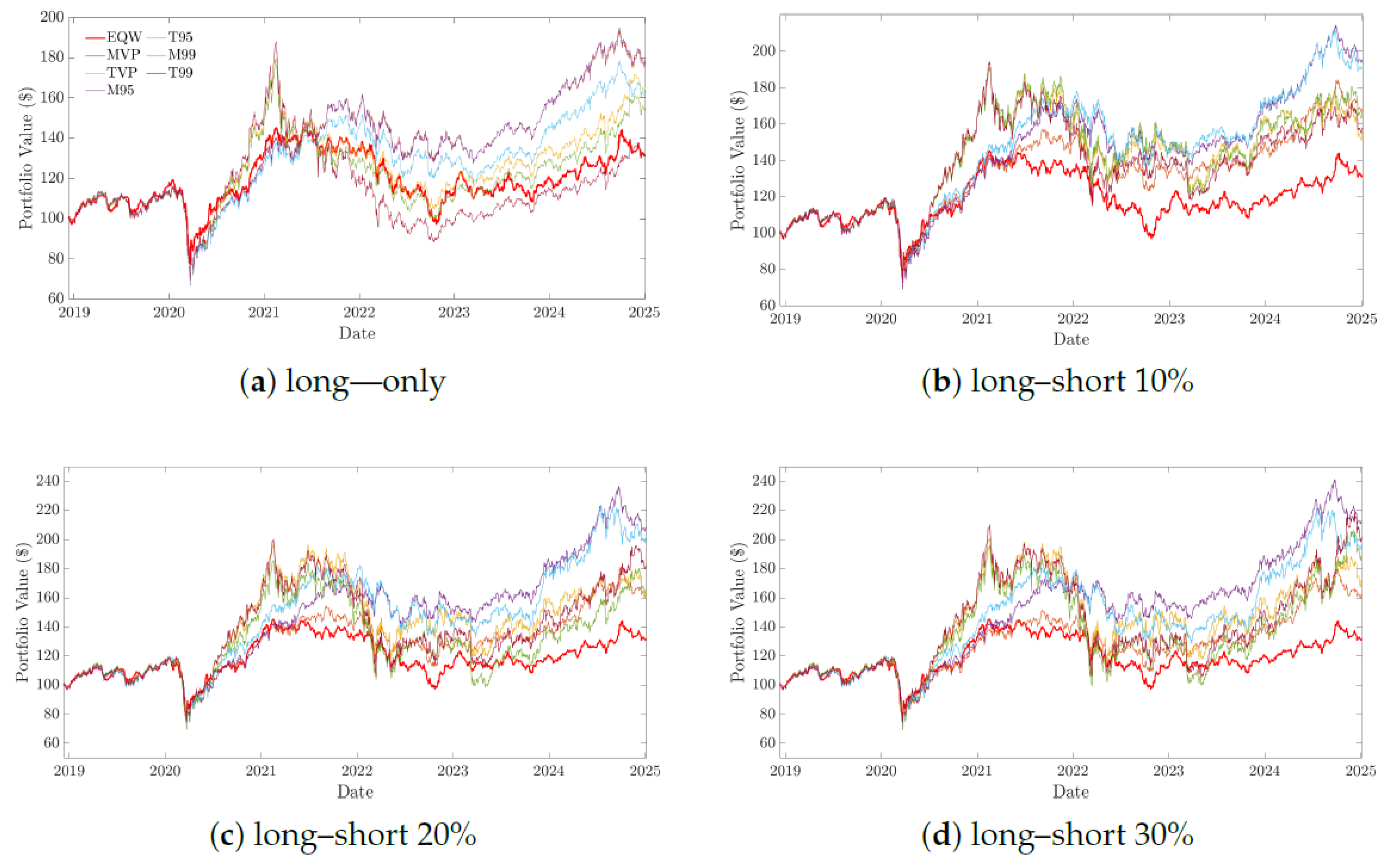
Across all strategies, the optimized portfolios consistently outperform the EQW benchmark over the full sample period, underscoring the value of systematic optimization in enhancing portfolio efficiency. This performance advantage is visible under both the long-only and long–short strategies, with the former delivering steadier, more risk controlled growth and the latter achieving higher cumulative returns by exploiting short positions. Although the EQW portfolio provides a simple, fully diversified allocation that does not rely on parameter estimates, the optimized portfolios systematically deliver higher terminal wealth and improved risk–return profiles, as illustrated in Figure 5. This supports the view that, for Asian and Asia-focused ETFs, moving from naive equal weighting to model based portfolio construction can generate economically meaningful gains.

Figure 5. Cumulative price performance of the optimized portfolios under long-only and long–short strategies from December 2018 to January 2025. The top panels display (a) the long-only strategy and (b) the long–short strategy with 10% leverage. The bottom panels correspond to long–short strategies with leverage levels of (c) 20% and (d) 30%. Each plot shows the growth of an initial USD 100 investment on 11 December 2018 over the analysis period.

Lindquist et al. (2021) note that the EQW portfolio is inherently long-only and is typically excluded from long–short analyses, but it is retained here as a consistent benchmark to illustrate relative performance across all strategies. The long-only strategy exhibits smoother trajectories with moderate gains, whereas the introduction of leverage in the long–short setting amplifies both returns and volatility. As leverage increases from 10% to 30%, portfolios experience progressively greater dispersion, demonstrating that while moderate leverage (10–20%) enhances performance without destabilizing the portfolio, higher leverage (30%) introduces pronounced fluctuations and sharper drawdowns during adverse market conditions. In the long-only strategy, M95 achieves the strongest terminal value, with T95, T99, TVP, and M99 clustered closely behind. Introducing short exposure and moderate leverage (10–20%) lifts the performance of the more return seeking portfolios (T95, T99, TVP), though at the cost of greater volatility. At higher leverage (30%), dispersion widens further as risk focused portfolios (M95, M99) maintain smoother growth and better downside resilience. Overall, leverage amplifies both returns and risks, with moderate levels improving performance efficiency and excessive leverage magnifying fluctuations and drawdowns.

From a practical perspective, these results have direct implications for different types of investors. Risk-averse investors, or those with binding regulatory or mandate constraints, are likely to prefer the minimum variance and minimum CVaR portfolios (MVP, M95, M99), which offer smoother growth and better protection against large losses, especially when leverage is low. In contrast, investors with higher risk tolerance may find the tangent and CVaR tangent portfolios (TVP, T95, T99) more attractive, since these portfolios target higher expected returns and stronger risk-adjusted performance, accepting greater interim volatility in exchange for improved long run outcomes. The long–short configurations with moderate leverage provide an additional tool for return enhancement, but our results indicate that the trade off becomes increasingly unfavorable at higher leverage levels, where tail risk and drawdowns rise sharply.

For global investors who currently hold primarily U.S. large cap or global market cap weighted benchmarks, our evidence suggests that optimized Asian ETF portfolios can improve performance relative to a naive equal weight allocation within Asia. However, we do not attempt a full allocation comparison across regions, and we only use the DJIA as a single developed market reference for tail behavior. A more complete assessment of whether Asian ETF portfolios are more or less attractive than U.S. or other regional ETF universes would require extending the analysis to include comparable multi region ETF datasets and joint optimization across continents, which is beyond the scope of this paper.

These findings directly address our third research question on the role of long-only versus long–short strategies and leverage in Asian ETF portfolios. The results show that long-only configurations provide smoother return paths and lower tail risk, while long–short strategies with moderate leverage (10–20%) improve performance on a risk-adjusted basis at the cost of higher volatility and more pronounced tail exposure. At higher leverage levels (30%), the deterioration in drawdowns and extreme losses dominates the incremental gains in average returns. This pattern implies that, for the Asian and Asia-focused ETF universe studied here, long–short strategies are most attractive when leverage is kept moderate, whereas highly leveraged positions are unlikely to be suitable for risk-averse investors or for portfolios with strict downside risk constraints.

4.3. Risk–Return Performance Evaluation

We evaluate the performance of the optimized portfolios (MVP, TVP, M95, T95, M99, and T99) under both the long-only and long–short strategies with leverage levels of 10%, 20%, and 30%. The EQW portfolio is included as a benchmark to assess the relative improvement achieved through optimization.

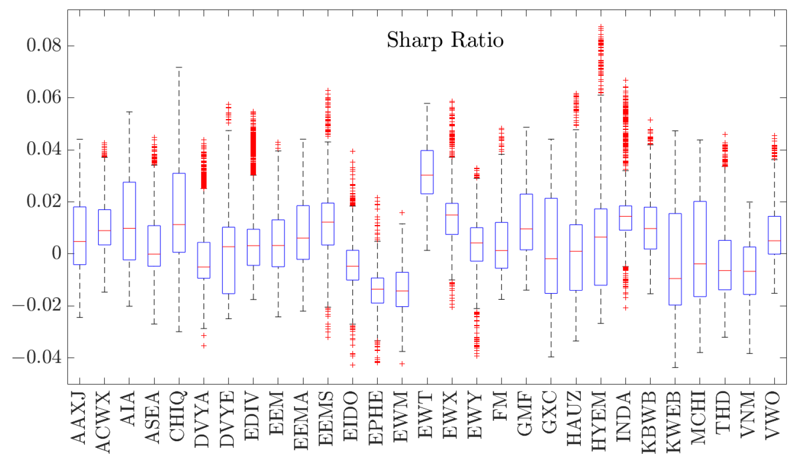
For a broader perspective, Appendix C presents boxplots of the Sharpe, STARR, and Rachev ratios for the 29 individual Asian ETFs. This highlights how each ETF performs on a risk-adjusted basis and complements the portfolio-level results reported here.

4.3.1. Sharpe Ratio Evidence (Volatility-Based Efficiency)

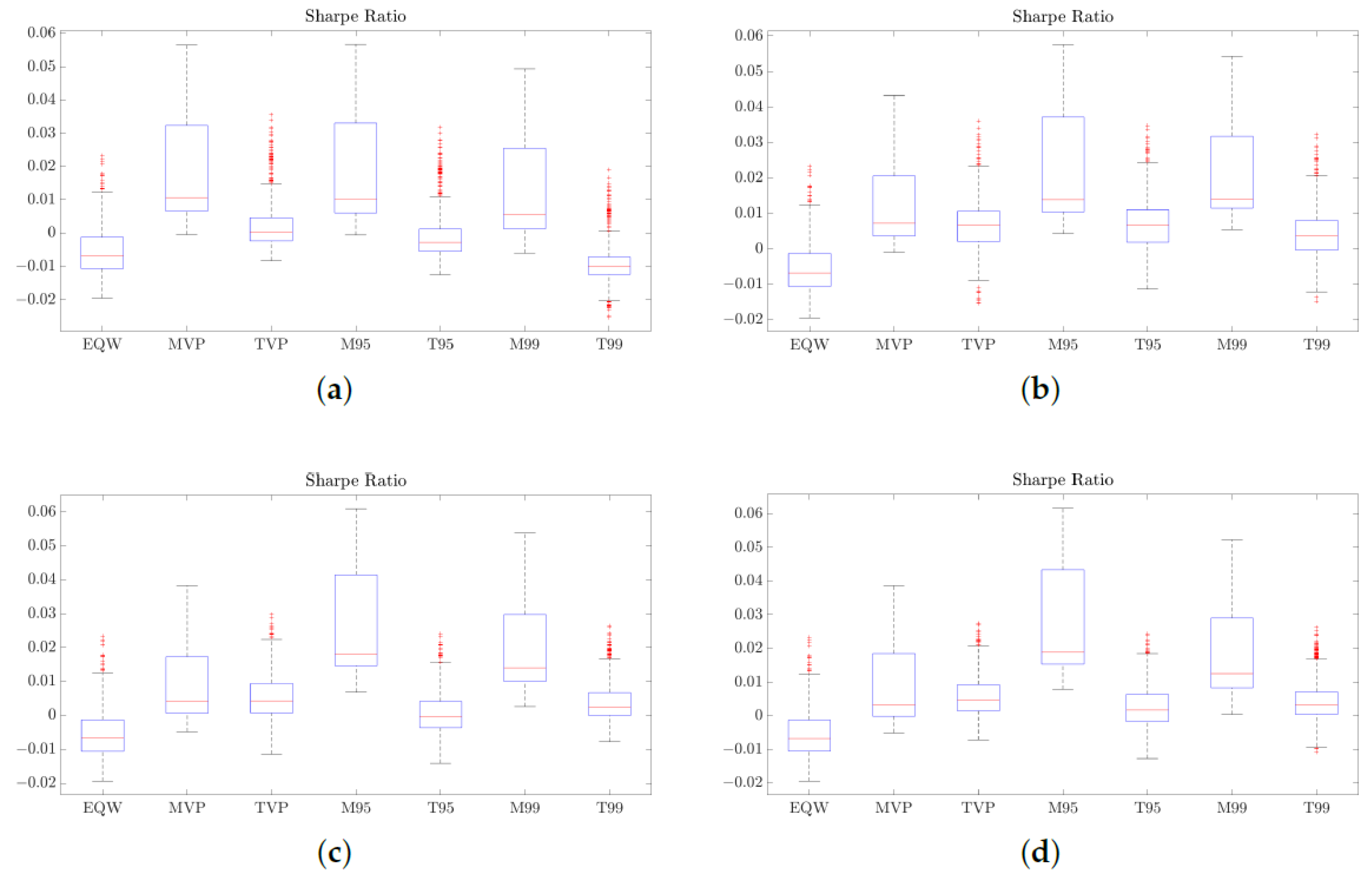
Figure 6 reports the Sharpe ratios of the optimized portfolios under the long-only and long–short specifications. In all configurations, the optimized portfolios tend to achieve higher Sharpe ratios than the EQW portfolio, confirming that systematic optimization improves the average reward per unit of total risk. Among the optimized strategies, the minimum-variance and minimum-CVaR portfolios (MVP, M95, M99) typically show the highest median Sharpe ratios. This is consistent with their construction: by explicitly minimizing variance or tail risk, these portfolios tilt towards the more stable ETFs in the universe and avoid the weakest performers, so that volatility in the denominator of the Sharpe ratio is reduced without sacrificing all of the available return premia.

Figure 6. Sharpe ratios of the optimized portfolios and EQW under long-only and long–short strategies. (a) Long-only. (b) Long–short 10%. (c) Long–short 20%. (d) Long–short 30%.

The tangent portfolios (TVP, T95, T99), which are designed to target higher expected returns, generally show Sharpe-ratio medians that are similar to or slightly below those of the minimum-variance and minimum-CVaR portfolios. These portfolios deliberately take on more exposure to volatile, return-seeking ETFs; when realized returns do not fully compensate for the additional risk, the Sharpe ratio is lower. Comparing the long-only panel with the long–short panels shows that allowing moderate leverage mainly increases the dispersion of Sharpe ratios rather than shifting the medians dramatically. Across portfolios, the median Sharpe ratios change only modestly when leverage is introduced, suggesting that leverage primarily magnifies outcome variability rather than systematically improving volatility-adjusted performance.

4.3.2. Rachev Ratio Evidence (Tail Asymmetry)

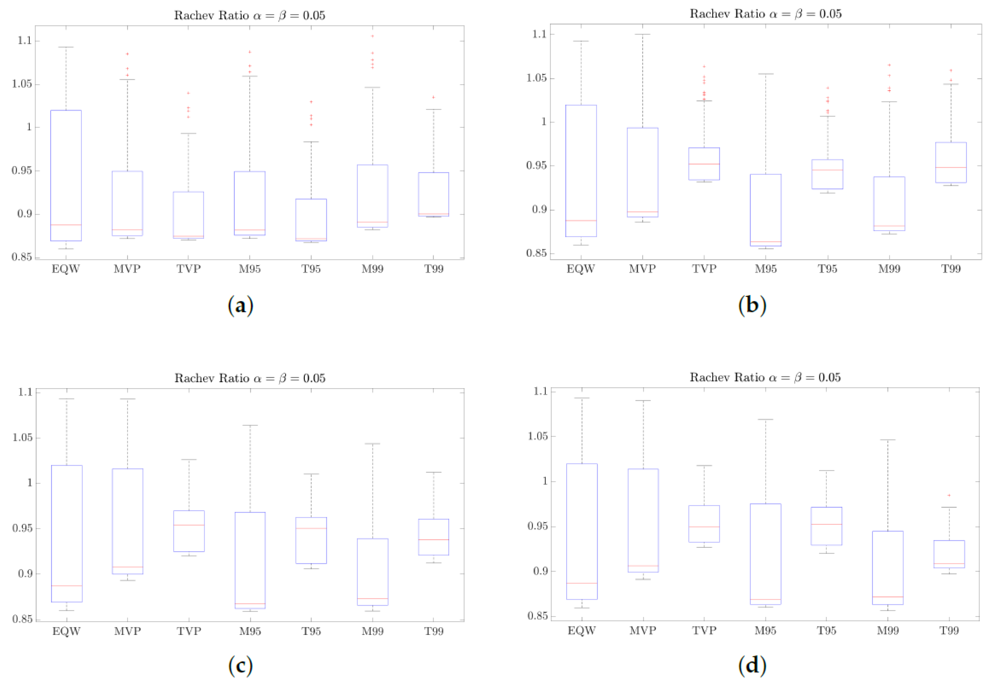
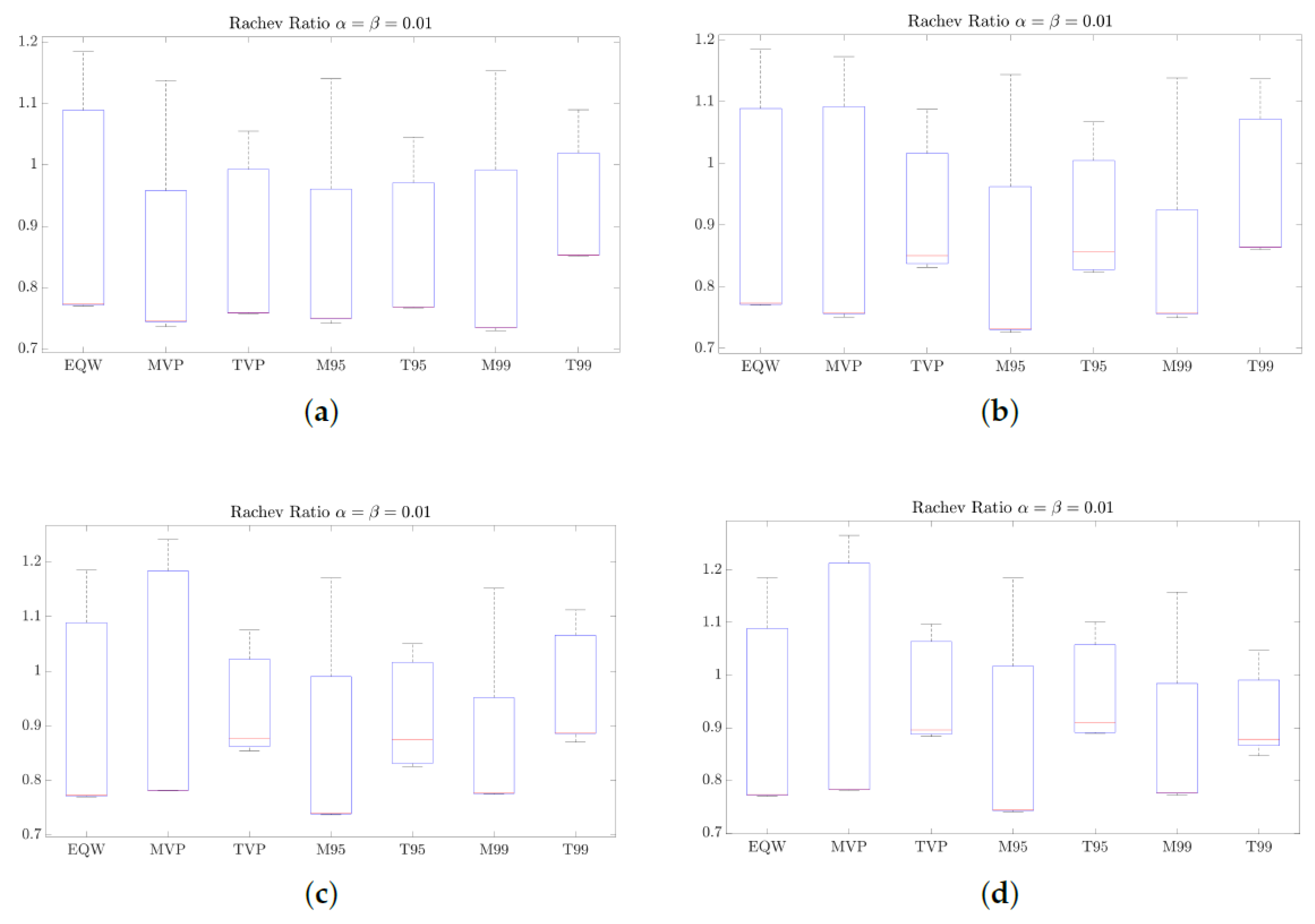
Figure 7 and Figure 8 show that Rachev ratio values for all portfolios remain within a relatively narrow band around unity. This suggests that none of the portfolios exhibits a persistent extreme imbalance between upside and downside tail outcomes. Comparing long-only and long–short configurations, the overall pattern of Rachev ratios is broadly similar across leverage levels. In several cases, particularly for EQW and the more return-oriented portfolios, the long–short variants display wider interquartile ranges, consistent with leverage amplifying both favorable and unfavorable tail realizations. Taken together, the Rachev results suggest that portfolios differ primarily in the dispersion of tail outcomes rather than in a systematic shift toward more favorable tail asymmetry.

Figure 7. Rachev ratio at the 95% confidence level for the optimized portfolios and EQW under long-only and long–short strategies. (a) Long-only. (b) Long–short 10%. (c) Long–short 20%. (d) Long–short 30%.

Figure 8. Rachev ratio at the 99% confidence level for the optimized portfolios and EQW under long-only and long–short strategies. (a) Long-only. (b) Long–short 10%. (c) Long–short 20%. (d) Long–short 30%.

4.3.3. STARR Ratio Evidence (Tail-Loss-Adjusted Efficiency)

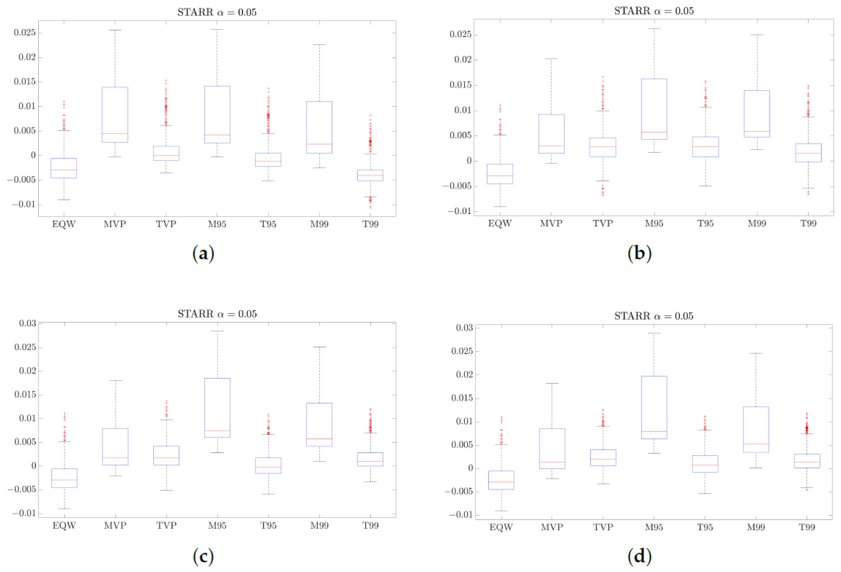
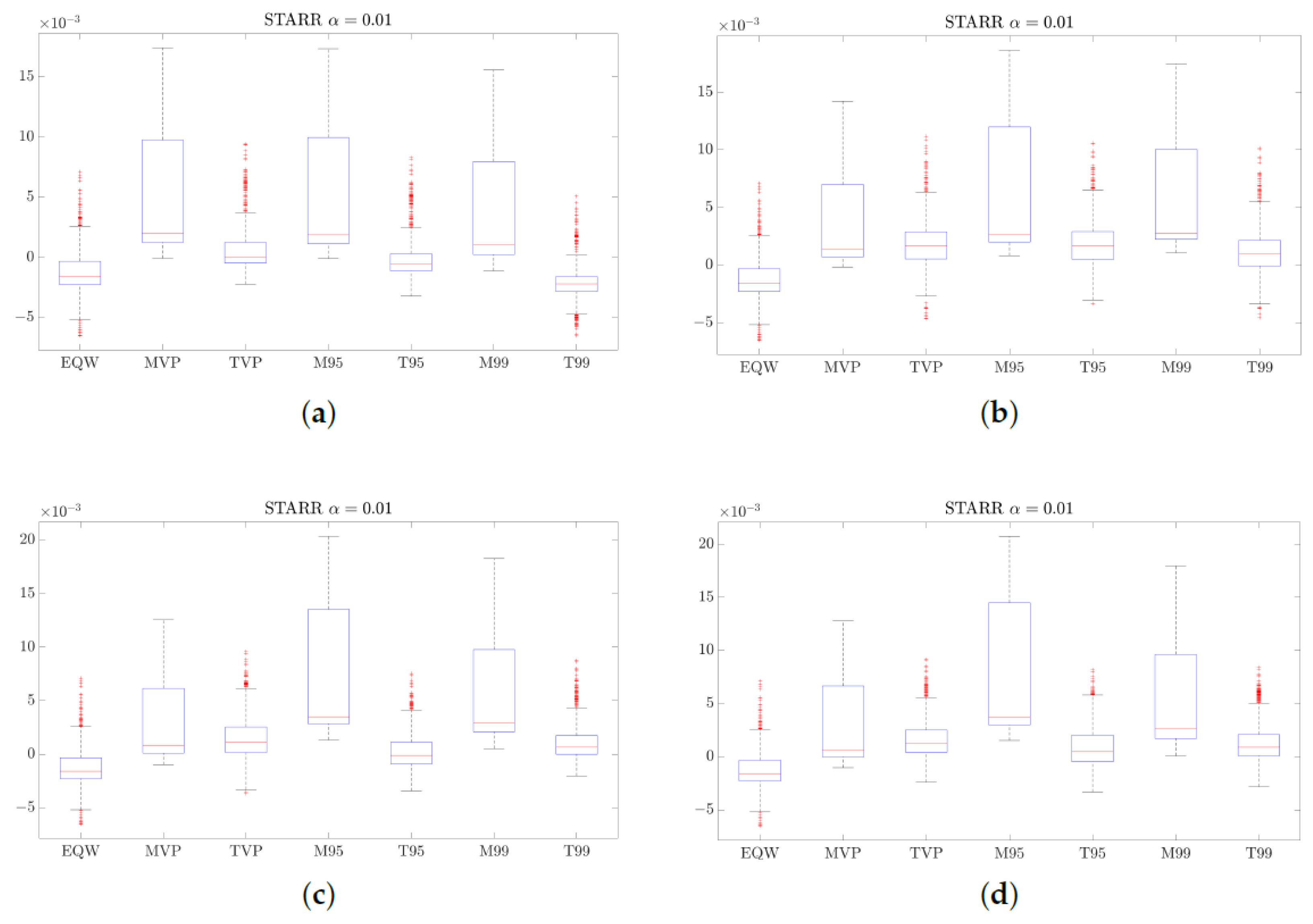
The STARR results in Figure 9 and Figure 10 broadly mirror the Sharpe patterns but place greater weight on downside tail risk. Across confidence levels and strategies, the optimized portfolios generally have higher median STARR values than EQW. The main exception is T99, whose median in the long-only case is close to that of EQW. This is consistent with the idea that, at such an extreme tail level, diversified long-only portfolios are all exposed to the same few market-wide crash days, so the optimizer has limited scope to distinguish T99 from the naive benchmark. Moving from the 95% to the 99% confidence level lowers median STARR values and increases dispersion across all strategies, reflecting the stronger influence of rare but severe losses on the denominator of the ratio.

Figure 9. STARR at the 95% confidence level for the optimized portfolios and EQW under long-only and long–short strategies. (a) Long-only. (b) Long–short 10%. (c) Long–short 20%. (d) Long–short 30%.

Figure 10. STARR at the 99% confidence level for the optimized portfolios and EQW under long-only and long–short strategies. (a) Long-only. (b) Long–short 10%. (c) Long–short 20%. (d) Long–short 30%.

4.3.4. Practical Interpretation

Portfolios that explicitly minimize variance or CVaR (MVP, M95, M99) tend to deliver higher and more stable risk-adjusted performance because their construction limits exposure to the most volatile and heavy-tailed ETFs, making large drawdowns less frequent and less severe. Tangent portfolios (TVP, T95, T99) intentionally tilt toward higher expected return segments, which can be advantageous in favorable markets but leads to more volatile ratios and greater sensitivity to extreme losses. Long–short strategies with moderate leverage can improve performance for several optimized portfolios, whereas higher leverage primarily magnifies tail dispersion and drawdown exposure without clear improvements in central risk-adjusted measures.

From a practical perspective, these patterns suggest that risk-averse investors, or those facing explicit drawdown or solvency constraints, may prefer the minimum-variance and minimum-CVaR portfolios, particularly in a long-only or low-leverage setting. Investors with higher risk tolerance may find the tangent portfolios more attractive, especially when combined with modest leverage, as they offer higher average returns at the cost of greater variability in both ordinary and tail outcomes.

5. Discussion

This paper provides an empirically grounded portfolio design and risk management analysis for Asian and Asia-focused ETFs. The objective is practical: to document tail-risk heterogeneity in a broad ETF universe, to show how variance-based and tail-sensitive optimization translate into implementable allocations, and to evaluate how long-only versus long–short constructions behave under bounded leverage. This positioning is consistent with a large empirical finance literature documenting that (i) ETF exposures can transmit liquidity shocks and affect the volatility and co-movement of underlying markets, and (ii) asset returns—especially in emerging-market and regionally concentrated settings—often exhibit non-normality and heavy tails, making downside-sensitive risk measurement economically relevant (Ben-David et al., 2018; Cont, 2001). Interpreted as a portfolio choice problem, our results connect data diagnostics, frontier estimation, and out-of-sample performance into a coherent economic narrative: the chosen risk measure materially changes portfolio composition and realized outcomes, and this sensitivity matters most when extreme downside events carry meaningful wealth and constraint costs.

A core contribution of the study is to clarify what efficiency means economically for investors rather than only mathematically. Efficient frontiers are not only feasibility boundaries; they represent menu-like choices among portfolio styles that map to real constraints and preferences. The minimum-variance portfolio corresponds to a volatility-control allocation suitable for mandates evaluated on stability, volatility targets, or tracking-error-type objectives. The CVaR-minimizing portfolios correspond to downside-protection allocations for settings in which losses in adverse states are binding (e.g., drawdown limits, risk-capital budgets, or margin-sensitive programs), consistent with the broader shift in risk management toward tail-aware criteria such as CVaR or expected shortfall (Acerbi & Tasche, 2002; Rockafellar & Uryasev, 2000). The tangent portfolios correspond to return-seeking allocations that maximize risk-adjusted performance under the chosen risk measure and risk-free proxy, and therefore align with investors willing to tolerate interim volatility and drawdowns in exchange for higher long-run efficiency. These interpretations are reflected in the cumulative wealth paths and the distribution of risk-adjusted ratios. In addition, our use of an equally weighted benchmark follows the empirical portfolio literature that treats simple $1/N$ allocations as an implementable baseline against which the incremental value of optimization must be evaluated out-of-sample (DeMiguel et al., 2009).

The emphasis on tail-sensitive methods is motivated by the descriptive tail diagnostics and by established evidence that financial returns can exhibit heavy tails and stress dependence, which make purely variance-based risk summaries incomplete in economically relevant states (Cont, 2001; Embrechts et al., 1997). The Hill tail-index comparison suggests that, over the region where the Hill curves stabilize, the equally weighted Asian ETF portfolio is associated with heavier tail behavior than the DJIA reference series in our sample. This result is used as a reference point rather than a definitive cross-market ranking because tail-index estimates can be sensitive to threshold choice, sampling variation, and dependence. The practical implication is therefore deliberately modest and implementable: extreme outcomes appear to play a more influential role in this Asian and Asia-focused ETF universe during the sample period, strengthening the case for complementing variance-based analysis with explicit tail-risk measures in portfolio construction and monitoring.

The comparison with the equal-weighted benchmark clarifies why optimization generates improvements in this dataset. The outperformance of optimized portfolios does not reflect a rejection of diversification; it reflects that equal weighting is not neutral with respect to tail risk when the asset universe contains meaningful heterogeneity in tail behavior and stress co-movement. Equal weighting mechanically assigns substantial weight to all segments, including those that contribute disproportionately to extreme losses. Optimization improves outcomes by reallocating away from persistently weak risk-adjusted contributors, exploiting diversification across heterogeneous exposures when dependence is imperfect, and reducing exposure to segments that amplify left-tail losses. Economically, this matters because the costs of tail events are not symmetric. Large drawdowns can trigger investor redemptions, margin calls, risk-limit breaches, and pro-cyclical de-risking, all of which can convert statistical tail risk into realized wealth losses and implementation frictions. In that sense, tail-sensitive optimization is not only a technical refinement but a direct response to the economic consequences of extreme downside events.

A further practical implication is that the optimization signal maps to observable, implementable instruments rather than remaining purely theoretical. The repeated proximity of EDIV to the tangent portfolios in both mean–variance and CVaR settings suggests that, within this universe and sample period, a dividend-oriented emerging-market ETF exhibits a risk-adjusted profile similar to that of the portfolio that maximizes efficiency under the relevant risk metric. The appropriate interpretation is not that EDIV is universally optimal, but that the characteristics favored by the optimizer can be approximated by readily available exposures. For investors constrained by turnover, operational complexity, or the ability to hold multi-ETF optimized portfolios, this provides a concrete example of how optimization outcomes can translate into implementable choices. It also highlights a broader point that is economically useful: in some regimes, portfolio efficiency gains can be obtained either through explicit optimization or through carefully chosen single-fund exposures that embed the same defensive or income-oriented characteristics favored by the optimizer.

The long-only versus long–short analysis extends the practical interpretation by showing how leverage changes the distribution of outcomes rather than only shifting average performance. Allowing short positions with moderate leverage can improve cumulative performance for several optimized portfolios, consistent with the idea that long–short flexibility can enhance efficiency by enabling within-universe hedging and relative positioning across ETFs. At the same time, leverage remains a double-edged tool. As leverage increases, dispersion widens and drawdowns become more pronounced, and the risk-adjusted ratio evidence indicates that leverage more reliably magnifies variability than it improves central performance. From a financial implementation perspective, this finding matters because higher leverage interacts with financing and margin conditions that tighten precisely during stress periods, when tail losses are most severe. The results therefore support a pragmatic policy for investors and risk managers: leverage should be treated as a risk-budget choice rather than a return target, and if leverage is used, moderate levels paired with downside-sensitive construction are more consistent with stable, implementable performance than aggressive leverage that primarily magnifies tail exposure.

The analysis also clarifies how hedging should be interpreted within the limits of an equity-heavy ETF universe. Because the dataset does not include classic defensive hedges such as Treasuries, gold, or explicit currency-hedged instruments, hedging is best defined as within-universe downside mitigation rather than absolute safe-haven behavior. Under this definition, an ETF has hedging characteristics if its inclusion tends to reduce portfolio downside during equity stress relative to a portfolio that excludes it. This can be evaluated using measurable criteria such as downside beta to a benchmark during benchmark drawdowns, conditional correlation in the worst benchmark return quantiles, or performance on the worst benchmark days. Within the current results, the most defensible inference is comparative: assets that receive weight repeatedly in tail-minimizing portfolios are candidates for downside-mitigating roles within the universe, while assets that dominate return-seeking tangent allocations are more plausibly pro-cyclical. For investors, the practical takeaway is that “hedging” in this setting should be interpreted as selecting exposures that reduce drawdowns within the Asian ETF opportunity set, not as substituting for traditional crisis hedges.

A broader implication of these results is that tail risk should be treated as a first-order input in portfolio monitoring and allocation design for Asian and emerging-market exposures. Because tail risk is time-varying and stress dependence can rise abruptly, tail-sensitive diagnostics and tail-sensitive portfolio construction can be integrated into periodic portfolio review processes, particularly when drawdowns rise, dispersion increases, or tail indicators deteriorate. At the same time, focusing on extremely rare tails at very high confidence levels can produce less stable comparisons because optimization becomes driven by a small number of shared crash observations. This does not reduce the usefulness of tail-sensitive measures, but it highlights the value of combining CVaR with complementary diagnostics such as drawdown measures and tail monitoring rather than treating any single metric as a sufficient summary of risk.

Beyond investor decision-making, the empirical patterns documented in this study also have policy-relevant interpretations for regulators and market overseers, especially in jurisdictions where ETF markets are growing quickly and are increasingly used by households and institutions as primary vehicles for international exposure. First, the evidence that tail outcomes are economically important in this universe supports the view that risk communication and disclosure frameworks should not rely solely on volatility-based metrics. Reporting drawdown and tail-loss statistics alongside traditional measures can better align disclosures with the risks that matter most during market stress, when investors are most likely to react and when liquidity conditions can deteriorate. Second, the leverage results underscore the importance of monitoring the interaction between leveraged strategies, margin conditions, and underlying-market liquidity. Even when leverage appears modest on paper, stress episodes can generate correlated selling pressure and widen price deviations, which can amplify volatility and increase systemic fragility. These implications are not causal claims derived from the data, but they are consistent with the risk patterns documented and provide a disciplined basis for discussing how portfolio design and market structure interact during stress.

This paper provides a clear foundation for several direct extensions. First, the analysis can be moved from frictionless to implementable by explicitly adding transaction costs, financing costs, and short-borrow costs, so that the reported portfolio improvements are evaluated on a net-of-cost basis. Second, the framework can be expanded beyond Asia by adding a small set of representative U.S. or global equity ETFs and at least one traditional defensive asset, which would allow the same variance- and CVaR-based methods to answer a simple allocation question: whether tail-aware Asian ETF portfolios improve the opportunity set of a global investor. Third, the downside-mitigation and hedging discussion can be made fully quantitative by reporting crisis-window behavior and conditional dependence measures, so that ETFs are identified as downside-reducing candidates using transparent criteria tied directly to drawdown reduction. These extensions are straightforward because they use the same optimization and evaluation machinery developed in this paper; they primarily expand the realism of implementation and the breadth of the investment universe, while keeping the focus on economically meaningful risk management under heavy tails.

6. Conclusions

This study analyzes 29 Asian and Asia-focused ETFs over 2014–2025 and evaluates whether variance-based and tail-sensitive optimization improves portfolio outcomes relative to a simple equally weighted benchmark. Using rolling-window estimation, we construct Markowitz and CVaR efficient frontiers and implement six optimized portfolios (MVP, TVP, M95, T95, M99, and T99) under long-only constraints and under long–short configurations with leverage levels of 10%, 20%, and 30%. Performance is assessed using the Sharpe ratio and tail-sensitive measures, including the Rachev and STARR ratios, supported by tail diagnostics based on the Hill estimator.

Across specifications, optimized portfolios dominate the equally weighted benchmark in risk-adjusted terms, confirming that systematic allocation improves efficiency in this ETF universe. The choice of risk measure is economically consequential: CVaR-based portfolios provide more explicit downside protection in a setting where tail behavior is salient, while tangent portfolios deliver higher return potential at the cost of greater variability. Leverage is beneficial only up to a point; moderate leverage (10–20%) can enhance cumulative performance, but higher leverage (30%) mainly increases dispersion and drawdowns without clear improvements in central risk-adjusted performance. A practical insight from the frontier analysis is that EDIV lies close to the tangent solutions in both the mean–variance and CVaR frameworks, suggesting that dividend-oriented exposures can approximate the risk-adjusted profile of optimized allocations within this sample.

Overall, the results emphasize that portfolio construction for Asian and emerging-market exposures should not rely on variance alone. Incorporating tail-sensitive risk measures provides a more robust basis for allocation and for periodic risk monitoring, especially when extreme downside outcomes are economically costly.

Finally, future work will extend this framework from historical rolling-window optimization to dynamic allocation rules that model time-varying returns, volatility, and dependence in Asian and Asia-focused ETFs. Using ARMA–GARCH-type dynamics with fat-tailed innovations and copula-based dependence structures, we will evaluate dynamic mean–variance and tail-aware policies out-of-sample on a net-of-cost basis under explicit financing and short-borrow constraints.