Abstract
This paper analyzes the effectiveness of some defensive assets inside global stock portfolios by applying a standard VaR approach to daily data from 2021 to 2024. The 5Y US note is by far the best hedging instrument for single-hedged portfolios, while in multiple-hedged portfolios further VaR reductions are obtained including commodities, utilities, and real estate stocks. Bitcoin’s hedging performance is strongly negative, displaying an average VaR difference of more than two basis points with respect to the best-performing multiple-hedged portfolio in moderately defensive scenarios. This gap implies much higher maximum potential daily losses for Bitcoin’s single-hedged portfolios. Dynamic risk profiles of multiple-hedged portfolios display a smoother pattern than single-hedged portfolios, particularly during turbulent periods corresponding to the start of the Russia–Ukraine war, emphasizing the crucial benefits of higher asset diversification.
JEL Classification:
C22; G15
1. Introduction and Motivation
Since Markowitz (1952) seminal contribution, the benefits of portfolio diversification have been widely acknowledged in the finance literature.
The mean-variance approach, which represents the cornerstone of Modern Portfolio Theory, laid the foundation for analyzing the risk/return relationship in a portfolio context, highlighting the benefits of diversifying investments across several asset classes in order to maximize expected return for a given risk level (or, alternatively, to minimize risk for a given level of expected return).
This approach is still widely used in order to implement optimal asset allocation strategies, notwithstanding some promising developments in the theoretical literature (see, e.g., Sears & Wei, 1985; Kimball, 1990) and in applied work relying on machine learning (e.g., Prayut & Sashi, 2019).
The first two decades of the current century witnessed a large number of financial crises, which prompted a huge research effort that was mostly aimed at establishing the hedging and safe-haven properties of various defensive assets.
Intense episodes of stock market turmoil and volatility persistence continued during the first half of the current decade, mainly as a result of Russia’s invasion of Ukraine in February 2022. Applied work exploring the role of defensive assets, therefore, also represented an important research catalyst during the first half of the current decade.
The properties of defensive assets were investigated through the standard R. Engle (2002) DCC model (e.g., Ghorbali et al., 2023), or similar econometric approaches (see, among others, Fakhfekh et al., 2023; Thi Thuy et al., 2024; Hanif et al., 2024). A parallel research line investigated the defensive properties of various candidate assets applying Wavelet Coherence Analysis (e.g., Belhassine & Riahi, 2025). Further research directions analyzed the role of geopolitical risk during more recent financial turmoil (e.g., Shaik et al., 2023), the relationships between volatility spillovers, defensive assets, and stock markets (e.g., Khan, 2025), and assessed the impact of the Russia–Ukraine conflict on financial markets through event study methodologies (see, among others, Boubaker et al., 2022; Yousaf et al., 2022).
Overall, a major drawback of these more recent studies is a scant attention to Value-at-Risk (VaR) measures for representative global stock portfolios, including a satisfactory number of potentially defensive assets.
Ullah et al. (2024) explore Bitcoin’s defensive role in the Russian financial market during the initial stage of the current Russia–Ukraine war. Dynamic correlations between Bitcoin and other financial assets (gold spot price, Moex stock index, Russian 1-year government bonds, and US Dollar/Ruble exchange rate) are computed through different Garch models, and risk analysis is performed by applying VaR and CVaR methodologies.
Although showing that Bitcoin represents a powerful hedging tool, this paper has several limitations. First, the analysis is exclusively focused on Russian financial assets and, therefore, does not reflect the perspective of a global investor. Second, Bitcoin is assumed as the only defensive asset, thus disregarding the effects of potentially more efficient risk-reduction strategies through multiple defensive assets. Third, VaR measures are not derived within a Multivariate Garch framework. Bitcoin’s defensive properties are examined in bilateral portfolios, including only one financial asset, thus neglecting potential risk-reduction gains associated with increased asset diversification.
Pivrnec (2024) focuses on the Russia–Ukraine war, investigating the defensive properties of various cryptocurrencies inside a portfolio including major world stock indexes (SP 500, Nasdaq 100, FTSE 100, Dax, Shangai Composite, and Nikkey 225).
The main result is that most cryptocurrencies denote a limited defensive role, with the exception of Tether.
The focus on a well-diversified portfolio, the evaluation of risk profiles based on different defensive strategies, and random weights portfolio replications are the main contributions of this research. However, the exclusive focus on cryptocurrencies represents one relevant drawback since, as widely documented in the literature, a large number of different assets may potentially provide risk-reduction improvements inside global stock portfolios (i.e., defensive stocks, precious metals, government bonds, and major international currencies).
This paper contributes to the existing literature by implementing an efficient VaR evaluation of global stock portfolios hedged through alternative defensive assets.
Drawing on the previous discussion, I focus on the early years of the current decade and propose a set of VaR indicators incorporating either single or multiple defensive tools in asset portfolios.
The benchmark unhedged portfolio includes stock indexes from the world’s most representative economic areas (US, Europe, India, China, and Japan), thus properly mimicking the perspective of a global international investor. Moreover, while retaining Bitcoin in order to compare our results with earlier findings, a large set of potential hedging assets is explored, including defensive stocks (health, commodities, utilities, and real estate sectors), precious metals (silver, palladium), and outstanding government bonds (5-Year US Note, 30-Year US Note).
The paper outline is as follows.
Section 2 describes the data set and performs a preliminary data inspection. Section 3 discusses the empirical evidence. I compare the benchmark unhedged portfolio with single-hedged (Section 3.1) and multiple-hedged (Section 3.2) portfolios. These results are evaluated not only in terms of average VaR values but also by focusing on the time-varying profiles of risk indicators, particularly with reference to more turbulent periods (Section 3.3). These high-volatility periods include, in addition to the beginning of the Russia–Ukraine war, some strong but short-lived turbulences during the second half of 2024, related to uncertainties about Japan’s (August 2024) and China’s (October 2024) macroeconomic perspectives. Section 4 concludes, summing up the main evidence and pointing out some directions for future research.
2. Data Set and Preliminary Data Inspection
The analysis relies on daily data from 29 March 2021 to 5 November 2024, yielding a total of 909 observations for each series.
The series list includes five aggregate global stocks and nine defensive assets.1
The former group, selected in order to accurately reflect a representative international investor’s perspective, comprises the following aggregate stock indexes: S&P500, Stoxx Europe 50, Shanghai Stock Exchange (SSE) Composite, Nikkei 300, and BSE Sensex.
The latter group includes a large variety of hedging and safe-haven assets, ranging from defensive sectors (health, utilities, and real estate) to precious metals (silver, palladium), one aggregate commodity index (Bloomberg), outstanding government bonds (5-year and 30-year US notes), and cryptocurrencies (Bitcoin).
Table 1 contains descriptive statistics of asset return series. The former section (Table 1A) refers to aggregate global stocks, while the latter (Table 1B) includes defensive assets.

Table 1.
(A) Stock price descriptive statistics for asset returns. (B) Defensive assets descriptive statistics for asset returns. Daily Data: 29 March 2021–5 November 2024 (908 Observations).
Average daily returns are always very close to zero. This finding is common in the literature, even at lower data frequencies (see, e.g., Tronzano, 2022), and supports the efficient market hypothesis.
Asset return variability is around 0.010 for global stocks, slightly lower for defensive stocks, as one would intuitively expect, and notably higher for Bitcoin (0.037). This last result is in line with recent research pointing out Bitcoin’s intrinsically speculative nature (Baur et al., 2018), notwithstanding some contributions which document its defensive properties during periods of financial turmoil.
Global stock returns are negatively skewed (except the Chinese stock index), pointing out asymmetric distributions with long tails in the leftward direction, whereas more variegated evidence characterizes defensive assets.
Positive excess kurtosis is a pervasive feature, thus capturing a well-known empirical regularity of asset returns, namely the existence of fatter tails relative to the normal density. Consistent with this result, the Jarque–Bera test strongly rejects the null hypothesis of normality for all series.
Strong Arch effects are apparent for stock returns at all lags. Quite similar evidence is documented for defensive assets, with minor exceptions (silver, US Treasuries). Overall, this evidence supports the use of a Multivariate Garch approach.
Mixed evidence stands out from serial correlation tests. Focusing on global stocks, the null of the absence of residual serial correlation is never rejected (except for the Japanese stock index), whereas more frequent rejections are recorded for defensive assets. Overall, this suggests that an AR(1) filter is appropriate in the context of this empirical investigation.
I now take a quick glance at the dynamic patterns of stock return volatilities. This preliminary inspection is a preview of the analysis in Section 3, where the risk-minimizing effects of defensive assets inside global stock portfolios will be explored.
Figure 1 reproduces conditional volatilities of stock returns.
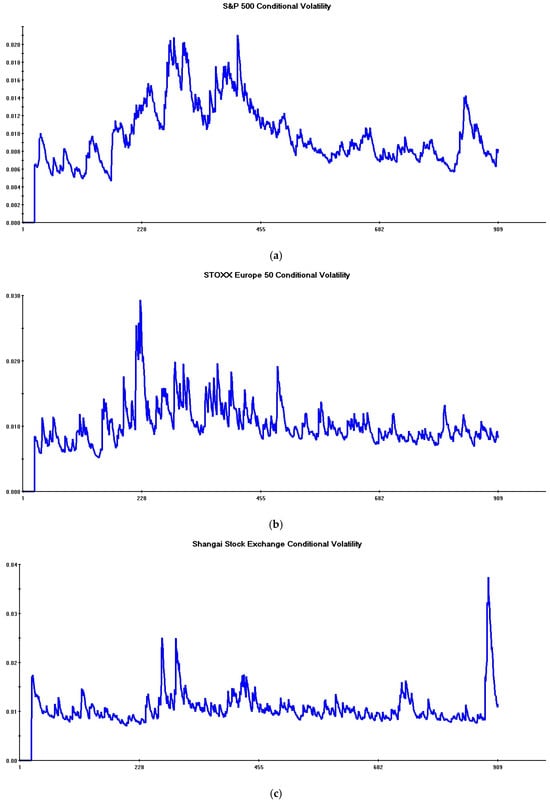
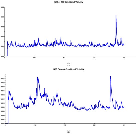
Figure 1.
Conditional volatilities of global stock returns (Daily Data: 29 April 2021–5 November 2024).
These volatility estimates are obtained from the “benchmark” Multivariate Garch model including only aggregate stock returns used in the next section.2
Major volatility spikes occur during the initial part of the sample and towards the end of the period.
The former turbulent phase occurs after a tranquil period on global stock markets, which extends from the starting date of volatility plots (end of April 2021) to the beginning of February 2022.
The regime switch in conditional volatilities occurred after the beginning of February 2022, when financial markets became fully aware of Russia’s imminent invasion of Ukraine. Note, for this purpose, the peculiar volatility pattern exhibited by European stocks, reaching record levels around mid-February, i.e., just one week before the start of the Russia–Ukraine war on 24 February 2022 (see Figure 1b). This movement is motivated by the major impact of this conflict on European firms and energy markets. This huge volatility increase quickly spread across all other stock markets (see Figure 1a,c–e). This major turbulent phase, corresponding to the start of the Russia–Ukraine conflict, dimmed around mid-July 2022.
The impact of war on return volatilities continued approximately until the end of October 2022. During this period, some temporary rebounds in European and US stock market volatilities are apparent, while Asian markets remained broadly unaffected. On the whole, these temporary rebounds are lower than upward pressures recorded during the initial months of the conflict.
A longer, more tranquil phase characterizes the second half of the sample. This phase is similar to the muted volatility pattern recorded in 2021, suggesting that, notwithstanding the prosecution of the Russia–Ukraine war, its destabilizing effects on global stock markets had been fully absorbed.
Towards the end of the sample, two short-lived volatility spikes are apparent.
The first, in August 2024 (see Figure 1d), is related to a sharp deterioration of investors’ sentiment in Japan, due to a strong Yen appreciation and uncertainties in the macroeconomic environment. The second, in October 2024 (see Figure 1c), reflects a depressed market sentiment in China, as a consequence of the lack of adequate fiscal stimulus in the presence of a fragile domestic consumption demand.
3. Empirical Evidence
3.1. Single-Hedged StockPortfolios
The cornerstone of the analysis is the seminal R. Engle (2002) DCC-Garch model. Since the features of this model are well-known, the reader is referred to the literature relying on this approach in regard to the decomposition of the variance–covariance matrix and details about parameter estimation.3
This model has been intensively used in the applied financial literature, since it is very flexible and computationally efficient in large systems. For these reasons, the DCC-Garch model represents the standard approach to compute dynamic conditional correlations, and is often preferred to other multivariate models such as the BEKK (R. F. Engle & Kroner, 1995) or the ADCC (Cappiello et al., 2006).4
Our benchmark specification is a version of the DCC-Garch model that includes five aggregate stock returns from major world economic areas (US, Europe, China, Japan, and India). This specification outlines an unhedged scenario, which does not incorporate any defensive asset inside a global stock portfolio.
This sub-section compares this benchmark with alternative single-hedged portfolios. Each portfolio includes only one defensive asset, while the comparison with the benchmark scenario is carried out in terms of average Value-at-Risk (VaR) values obtained over the full sample period.5
The specification of this model is consistent with preliminary data inspection.
Section 2 documents the existence of residual serial correlation at various lags in one stock return series (i.e., Japanese stocks, see Table 1A), while significant rejections of the null of absence of serial correlation are recorded for many defensive assets (see Table 1B). All return series are, therefore, pre-filtered with an AR(1) process before proceeding to model estimation. Residual plots of pre-filtered series suggest that they are white noise, and all estimated models rely on these pre-filtered data.
Further peculiar features documented in Section 2 are the existence of positive excess kurtosis and strong rejections of the null of normality for asset returns. The existence of fat tails and significant departures from normality suggests estimating Multivariate Garch models following the t-DCC specification proposed in Pesaran and Pesaran (2010).6
R. Engle (2002) DCC model allows for separate specifications of parameters driving conditional volatilities and conditional cross-correlations of asset returns.
In all estimated models, conditional volatility parameters are left unrestricted and are assumed to be different for each variable. As regards conditional cross-correlation estimates, a common structure is imposed for variables appearing inside each model. In most models, moreover, the autoregressive parameter driving asset correlations is restricted in order to achieve convergence in the estimation algorithm.7
For all models, the first 20 observations are used to initialize recursions and compute standardized returns based on rolling historical volatilities. These Multivariate Garch models are thus based on 887 daily observations from 29 April 2021 to 5 November 2024.
The Maximum Likelihood algorithm converges after 41 iterations in the case of the benchmark model, whereas the remaining models require more iterations in order to reach convergence (55 iterations, on average).
The validity of the t-DCC specification is assessed using the diagnostic tests suggested in Pesaran and Pesaran (2010). The null hypothesis of correct model specification is never rejected, at standard significance levels, neither by a Lagrange multiplier test for serial correlation in probability transform estimates, nor by the Kolmogorov–Smirnov statistic testing the uniformity of the distribution of probability transform estimates.8
Since the focus of this study is on the hedging properties of various defensive assets, parameter estimates are not reported in order to save space.9
Table 2 summarizes the results. The first column refers to the benchmark unhedged scenario, whereas VaR values relative to hedged portfolios are collected in the remaining entries.
Table 2.
Average Value at Risk (VaR) in single-hedged stock portfolios. DCC models estimated on daily data: 29 April 2021–5 November 2024. (VaR Confidence Level: 1%).
For each hedged portfolio, three simulations are considered.
In the first one (first row), each asset receives the same weight; therefore, as indicated in Table 2, each global stock and each defensive asset has the same weight (16.6%).
The second case (second row) represents a moderately defensive scenario, where the defensive asset weight is higher (30%), and global stock weights are correspondingly reduced. The third case (third row) represents a strongly defensive scenario, where the defensive asset weight is further increased (50%), and global stock weights are correspondingly further lowered.10
The former column in Table 2 displays the unique VaR value corresponding to the benchmark scenario, while the remaining columns report the risk-minimizing properties of various defensive assets. More specifically, from left to right, these columns start with single-hedged portfolios exhibiting the highest VaR values and progressively move towards portfolios exhibiting better risk-minimizing properties.
Consider, for this purpose, the first group of defensive instruments (Bitcoin, palladium, silver, and 30Y US note). A peculiar feature of this group is that all defensive assets yield values consistently higher than the benchmark, thus failing to deliver, during the period considered, positive risk-hedging features. This is particularly evident as regards Bitcoin and palladium.
A further destabilizing effect associated with this group is that an increase in defensive asset weights leads to increases in average portfolio risks. Once again, this is particularly evident as regards Bitcoin and palladium (see second and third row).
Consider now the latter defensive asset group (health, commodities, utilities, and real estate stocks).
An improvement in the risk-minimizing properties is now apparent, although this beneficial effect is not substantial. In the “Equal Weights” simulation, a modest VaR improvement is recorded with respect to the benchmark scenario. This improvement involves all hedging instruments and exceeds 100 basis points in the case of real estate defensive stocks. Additionally, in line with previous results, progressively more defensive weight simulations lead to risk increases in all single-hedged stock portfolios.
Consider, finally, the last column of Table 2, which summarizes the hedging properties of the 5Y US note.
Focusing on the “Equal Weights” scenario, this defensive asset yields the best result in terms of VaR reduction with respect to the benchmark portfolio (see last column of Table 2, first row). Differently from previous results, a higher weight of this defensive asset never exerts destabilizing risk effects. A moderately defensive scenario yields a lower average VaR level (0.0092), which becomes significantly lower in the case of a strongly defensive scenario (0.0086).
To summarize, this empirical evidence reveals that only a limited number of financial instruments displays better risk-stabilizing properties than the benchmark portfolio.
Focusing on the “Equal Weights” scenario, only real estate defensive stocks and the 5Y US note yield significantly better results.
The 5Y US note, finally, stands out as the only defensive asset that does not exert destabilizing effects, since an increase in its weight inside global stock portfolios is associated with progressively significant risk reductions.11
3.2. Multiple-Hedged Stock Portfolios
As documented in the previous section, a benchmark portfolio incorporating only major global stocks is difficult to beat through single defensive assets, since only a limited number of them displays risk-minimizing properties. A natural question then arises: can an appropriate mix of defensive assets provide further risk improvements over this benchmark?
This section addresses this topic, building on some basic results obtained in Section 3.1.
Since the former group of defensive assets analyzed in Table 2 (Bitcoin, palladium, silver, and 30Y US note) fails to deliver risk-hedging benefits, this group is now excluded. I focus, therefore, on financial assets belonging to the second group (health, commodities, utilities, and real estate stocks), and the 5Y US note.
I consider five alternative multiple-hedged stock portfolios, where the 5Y US note is always included (being the top-performer on the basis of previous evidence).
More specifically, the following multiple-hedged simulations are considered:
- Five Defensive Assets: health, commodities, utilities, real estate stocks, and 5Y US note;
- Four Defensive Assets: commodities, utilities, real estate stocks, and 5Y US note;
- Three Defensive Assets: utilities, real estate stocks, and 5Y US note;
- 2A: Defensive Assets: utilities and 5Y US note;
- 2B: Defensive Assets: real estate and 5Y US note.
This selection reflects the role of various defensive assets explored in Section 3.1 in driving average VaR results reported in Table 2.
In line with the previous analysis, three scenarios are explored.
In the former “Equal Asset Weights” scenario, each asset has the same weight in a given hedged portfolio.12 In the latter “Moderately Defensive” scenario, the total weight assigned to defensive assets is 50%. All weights, both for single defensive assets and for single global stocks, are then equally split. In the “Strongly Defensive” scenario, the total weight assigned to defensive assets is increased to 60%, while single weights for both asset categories are equally split again.
Table 3 summarizes the empirical evidence.
Table 3.
Average Value at Risk (VaR) in multiple-hedged stock portfolios. DCC models estimated on daily data: 29 April 2021–5 November 2024. (VaR Confidence Level: 1%).
The first column refers to the benchmark portfolio, which, by construction, is identical to that analyzed in previous simulations. The remaining columns report the results for multiple-hedged portfolios, starting from those with the largest number of defensive assets and moving towards those with a lower number of them.
Consider the first row of Table 3, corresponding to the “Equal Asset Weights” simulation.
Differently from Section 3.1, all multiple-hedged portfolios beat the benchmark since the worst group of defensive assets has now been excluded.
Focusing on the best group of defensive assets previously identified (health, commodities, utilities, real estate, and 5Y US note), a crucial feature is that, under the “Equal Weights” assumption, the risk-minimizing properties of multiple-hedged portfolios are consistently better than those of the corresponding single-hedged portfolios. In other words, under the same weight assumption, multiple-hedged portfolios yield consistently lower average risk values than single-hedged portfolios.
This result provides strong support for Markowitz (1952) argument about the benefits associated with asset diversification.
Focusing again on the “Equal Weights” scenario, the best results are obtained when the number of defensive assets is relatively large. More specifically, the 4-Defensive portfolio yields the best average VaR result (0.00851), whereas both 2-Defensive portfolios exhibit worse hedging properties. Overall, this empirical evidence again lends robust support to Markowitz (1952) argument.
Moving towards stronger defensive portfolios, the “Moderately Defensive” scenario provides significant VaR decreases with respect to previous results in (almost) all cases (see Table 3, second row).13
The ranking of best hedged portfolios remains identical to that previously recorded. More specifically, the 4-Defensive asset portfolio again obtains the lowest VaR value (0.00843), followed by the 3-Defensive asset portfolio, whereas less-diversified portfolios display less favorable hedging properties14.
On the whole, therefore, the benefits from higher asset diversification are fully confirmed assuming a more prudential asset management strategy.
Quite interestingly, further increases in the weight of defensive instruments are no longer associated with lower portfolio risks. As shown in Table 3 (last row), the “Strongly Defensive” scenario actually has mild negative effects, slightly increasing all VaR values. This suggests that, beyond a given defensive asset threshold, the relationship between defensive asset weights and portfolio riskiness may actually become nonlinear.
Taken as a whole, the empirical evidence obtained so far points out that the best VaR values are obtained with the 5Y US note (0.0086: single-hedged, strongly defensive scenario) and with the 4-Defensive Asset combination (0.00843: multiple-hedged, moderately defensive scenario).
Since the difference between these values is small, it could be argued that, if a portfolio manager is able to pick up the best hedging tools, it does not make much difference whether you rely on single or multiple-hedged portfolios.
This conclusion is actually wrong, not only because it is obviously very difficult to pick up ex ante the best defensive assets. What matters are indeed not only average VaR values, but also the dynamic patterns of these risk indicators over time, particularly during highly turbulent periods.15
This issue is discussed in more detail in the next section, where some graphical evidence is provided in order to reaffirm the superiority of multiple-hedged over single-hedged portfolios.
3.3. Dynamic VaR Patterns: Some Comparisons
The previous sections analyzed average VaR patterns of single-hedged and multiple-hedged portfolios. In the present section, I complement this empirical evidence by providing some comparisons between the dynamic patterns of these indicators.16
A strong empirical regularity of financial data is the clustering of alternative volatility regimes of asset returns. This regime-switching process between “high” and “low” volatility periods is often due to the occurrence of financial crises, but may also depend on strictly exogenous events, changes in the macroeconomic environment, or changes in the risk appetite of economic agents.
As discussed in Section 2, visual data inspection documents four “high” volatility regimes during the period examined: the former two related to the outbreak of the Russia–Ukraine war, and the latter two induced by a deterioration of the macroeconomic outlook.
From an asset allocation perspective, it is, therefore, important not only to compute the average stabilizing properties of defensive assets over the whole sample but also to assess their risk-minimizing properties during particularly turbulent periods. As shown in Baur and McDermott (2010) and Baur and Lucey (2010) seminal papers, this task can be performed in a linear regression framework, discriminating between the hedging and safe-haven properties of defensive assets.
Drawing on the approach taken in the present paper, there is an alternative way to deal with this issue, which motivates the analysis carried out in the present section. More specifically, the VaR evidence from various hedged portfolios can be compared with that of the benchmark scenario, with a specific focus on dynamic risk profiles during high-volatility periods.
Further complementary motivations for the analysis performed in this section include a better understanding of the effects induced by an increase in defensive asset weights and a more accurate evaluation of the empirical evidence related to the best-performing portfolios.
It may be useful to start with a VaR comparison between the best- and worst-hedged portfolios.
This information is reproduced in Figure 2, where the upper plot refers to the multiple-hedged portfolio including four defensive assets (best results) and the lower plot refers to the single Bitcoin-hedged portfolio (worst results).
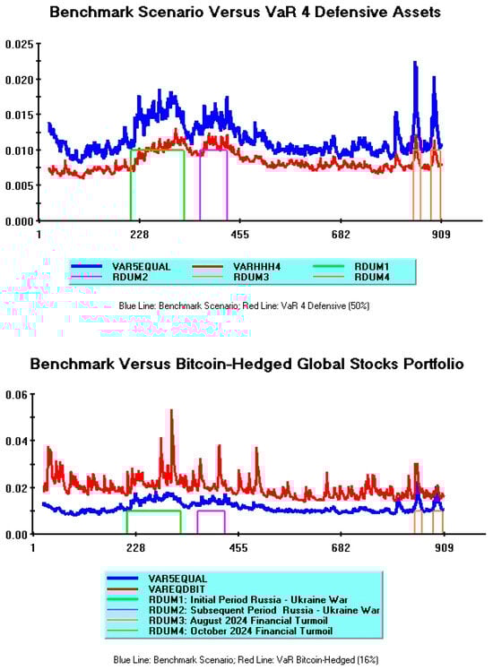
Figure 2.
Comparison between best and worst hedged portfolios.
Red lines in both plots refer to hedged portfolios (where a 50% defensive scenario is assumed for the multiple-hedged portfolio and an equal weights scenario is assumed for the single-hedged portfolio); blue lines refer instead to the benchmark scenario.17
A crucial feature of Figure 2 is that the blue line in the upper plot is always above the red line, whereas a reverse situation holds as regards the lower plot. This means that the former portfolio always beats the benchmark, whereas the latter never beats the benchmark.
Further relevant differences stand out, focusing on various turmoil periods (respectively, marked as green, violet, orange, and yellow rectangles).
The Bitcoin-hedged portfolio exhibits strong upward VaR spikes during high-volatility periods corresponding to the Russia–Ukraine conflict (green and violet lines); further upward, although less intensive, spikes are observed during the latest turmoil (orange and yellow lines).
Overall, therefore, the disappointing Bitcoin performance as a defensive asset documented in Section 3.1 is strongly corroborated by this empirical evidence.
Turning to the multiple-hedged portfolio, a persistent and significantly lower VaR is apparent with respect to the benchmark scenario.
The overall VaR pattern is much smoother than the Bitcoin one, with no significant spikes, thus signaling stable and robust risk-minimizing properties.
These positive hedging features are best appreciated during the instability phases characterizing the Russia–Ukraine conflict.
Focusing on the beginning of the war (green line), a remarkable VaR stability is observed, thus pinpointing significant decorrelations of the 4-Defensive Assets constituents from global stock returns volatilities. This positive hedging effect persists during the latter turmoil phase (violet line), although with slightly less intensity.
Finally, the end-of-period volatility jumps induced by Asian countries’ macroeconomic instabilities are reflected in two upward VaR spikes (orange and yellow lines). These risk increases, however, are notably lower than those recorded under the benchmark scenario (i.e., they are approximately around 0.012) and, consequently, are also much lower than those recorded for the Bitcoin-hedged portfolio during corresponding turmoil periods (which are approximately around 0.03).
Section 3.1 documents that Bitcoin belongs to the first group of defensive instruments failing to deliver, on average, appreciable risk-hedging effects.
Figure 3 offers further empirical evidence on this matter, analyzing dynamic VaR patterns of the remaining components of this group (palladium, silver, and 30Y US note).
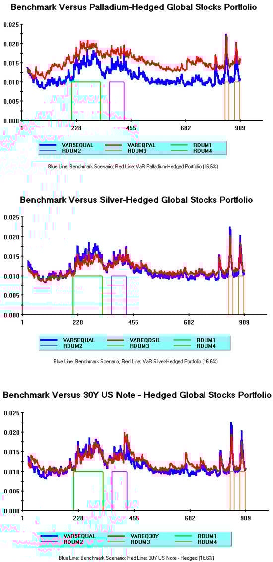
Figure 3.
Benchmark scenario versus palladium, silver, and 30Y US note-hedged portfolios.
The palladium-hedged portfolio (upper red plot) is quite similar to Bitcoin. The VaR indicator, although displaying fewer upward spikes, is consistently above the benchmark.
Risk profiles appear significantly better in the remaining two cases: actually, both silver (center red plot) and the 30Y US note (lower red plot) VaRs indicators overlap the benchmark, thus displaying a “neutral” situation where the defensive assets’ role is basically irrelevant.
Note, however, that, during the former turmoil associated with the Russia–Ukraine war (green line), the VaR of the silver-hedged portfolio remains slightly under the blue line, thus displaying a modest risk-hedging effect.
Overall, while confirming the ranking of worse defensive assets documented in Section 3.1, Figure 3 highlights the different hedging features provided by some of these assets during major financial turmoil.
Let us now explore in more detail the latter group of defensive instruments, namely, multiple-hedged portfolios.
Figure 4 compares Var from a multiple-hedged portfolio including four defensive assets (5Y US note, commodities, utilities, and real estate) with that of a portfolio including a reduced number of these assets (5Y US note and utilities). In both cases, VaR simulations (red lines) assume a 50% defensive scenario, while the blue line again refers to the benchmark scenario.
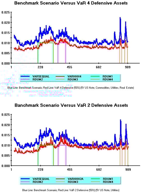
Figure 4.
Multiple-hedged portfolios: A comparison.
Overall, these two VaR patterns and their variability are quite similar, particularly during the initial and the final part of the sample.
Some significant differences are instead apparent during turmoil periods related to the Russia–Ukraine conflict. During these “high volatility” phases, the less-diversified portfolio denotes a larger instability and more frequent upward spikes towards the benchmark (see red line in the lower plot, and green and violet lines delimiting these turbulent periods).
This evidence pinpoints the drawbacks (advantages) of a lower (higher) asset diversification during major turbulent periods, which is closely in line with Markowitz (1952) main argument.18
Let us now focus on the effects of an increase in defensive asset weights.
Figure 5 explores these effects, comparing the best single-hedged portfolio, including the 5Y US note as a defensive asset (upper plot), and the best multiple-hedged portfolio, including four defensive assets (lower plot).
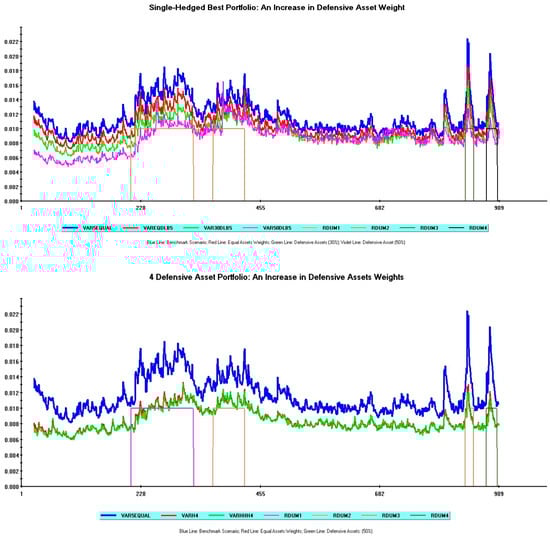
Figure 5.
Effects of an increase in defensive asset weights in best single-hedged and multiple-hedged portfolios.
The blue line corresponds to the benchmark scenario in both plots. The remaining lines report the Equal Asset Weights scenarios (red lines in both plots) and the downward shifts in VaR values generated by more defensive portfolios. For the single-hedged portfolio, a shift to a 30% defensive scenario (green line) and a further shift to a 50% defensive scenario (violet line) are shown. For the multiple-hedged portfolio, only a shift to a 50% defensive scenario (green line) is shown.
Consider the single-hedged portfolio. As documented in Figure 5 (upper plot), the shift towards more defensive scenarios generates appreciable hedging effects, namely a significant drop of risk indicators from the benchmark, particularly during the first turmoil period related to the beginning of the Russia–Ukraine conflict.
Consider now the 4-Defensive Asset Scenario. In this case, as documented in Figure 5 (lower plot), the risk improvement is almost always negligible.
This difference is easily understood as reflecting the greater impact of a defensive asset’s weight increase inside a single-hedged portfolio than inside a multiple-hedged portfolio. In the former case, the increase in defensive asset weights starting from an Equal Asset Weights portfolio corresponds to an increase from 16.6% to 50%. In the latter case, the corresponding increase is instead only from 44.4% to 50%.
The negligible risk-minimizing gain observed for the 4-Defensive Assets portfolio dependson the fact that the bulk of hedging effects stems from the pre-existence of a large component of defensive assets associated with the underlying diversification strategy.19
This section is concluded by discussing the issue raised at the end of Section 3.2: if the Average VaR gap between two hedged portfolios is very small, does it make any difference which portfolio is actually chosen?
In the context of this paper, these portfolios are represented by the best single-hedged (relying on the 5Y US note as a defensive asset) and by the best multiple-hedged (relying on four defensive assets) portfolios.
Figure 6 plots these time-varying VaR patterns, assuming in both simulations a 50% weight for defensive assets. In this figure, the blue line corresponds to the single-hedged portfolio, while the red line corresponds to the multiple-hedged portfolio.
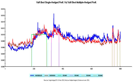
Figure 6.
Best single-hedged Vs/best multiple-hedged global stock portfolios: A Value at Risk comparison.
The single-hedged portfolio prevails, in terms of lower VaR values, during the initial part of the sample. During the earlier phase of Russia–Ukraine conflict (green lines), the risk performance of these portfolios is broadly similar. However, during the latter major “high volatility” phase (violet lines) and the following long-lasting tranquil period, the more diversified portfolio definitely displays better risk-minimizing properties. During the latest short-lived turmoil periods, VaR patterns are broadly identical.
Therefore, although these portfolios yield quite similar average VaR values, the advantage provided by the multiple-hedged one is represented by a smoother and less variable pattern during the sample period.20
Assuming a standard mean-variance framework, this implies that a representative investor’s utility is higher by selecting the multiple-hedged portfolio, thus reiterating a robust support of Markowitz (1952) main argument about diversification benefits.
4. Concluding Remarks
The mean-variance framework, originating from Markowitz (1952) seminal contribution, still represents a cornerstone in the applied financial literature dealing with portfolio selection, optimal asset diversification, and VaR evaluation.
While this approach was intensively used during the first two decades of the current century in order to explore the defensive properties of a large number of assets, some relevant pitfalls characterize more recent work focusing on the first half of the current decade.
More specifically, VaR indicators have not yet been exhaustively explored in this latest strand of literature, since existing contributions either do not reflect an international investor’s perspective or neglect a large number of defensive assets.
This paper takes a first step towards fixing the above drawbacks.
Improving upon previous contributions, five major aggregate stock indexes are selected (S&P 500, Stoxx Europe 50, Shanghai Stock Exchange (SSE) Composite, Nikkei 300, and BSE Sensex). Moreover, differently from previous work, the focus is on a large number of hedging assets, ranging from defensive sectors to precious metals, one aggregate commodity index, outstanding government bonds, and Bitcoin.
The empirical findings may be summarized as follows.
A first round of DCC-Garch estimates assuming single-hedged stock portfolios reveals a sharp difference between various defensive assets.
A former group of assets is quite heterogeneous (Bitcoin, precious metals, and 30Y US note) and consistently fails to deliver positive risk-hedging features. Average VaR values associated with this group are always higher than those obtained from an unhedged benchmark portfolio including only aggregate global stocks. Moreover, increasing these asset’s weights to 30% or 50% in order to simulate stronger defensive scenarios, average VaR values consistently increase above the benchmark, pointing out significant destabilizing effects.
A second group of hedging instruments, including one aggregate commodity index and various defensive stocks (health, utilities, and real estate), provides modest risk-reduction improvements. Assuming “Equal Assets Weights”, average VaR values are, in most cases, slightly lower than the benchmark. Moreover, focusing on more-defensive single-hedged portfolios, destabilizing effects still persist, suggesting that even this group does not perform well enough in terms of risk reduction.
A third group includes only one asset, namely the 5Y US note.
Assuming “Equal Assets Weights”, a modest improvement with respect to the benchmark is recorded. However, significant VaR reductions are obtained by simulating more-defensive scenarios, which is different from previous results.
Overall, therefore, the 5Y US note stands out as the most effective defensive asset among single-hedged stock portfolios.
Building on this evidence, the analysis is extended to multiple-hedged stock portfolios, excluding the former group of defensive assets given their unsatisfactory performance.
Five multiple-hedged portfolios are explored, progressively reducing the number of hedging instruments. In line with the previous analysis, the unhedged benchmark is compared with alternative simulations mimicking different degrees of risk protection.
All multiple-hedged portfolios significantly beat the benchmark.
The best-performing portfolio includes four defensive assets: 5Y US note, commodities, utilities, and real estate stocks. Assuming a moderately defensive scenario, where the total weight of defensive assets amounts to 50%, this portfolio yields the best risk-minimizing results, while further increases in hedging asset weights do not bring additional risk reductions.
The average VaR value of the best multiple-hedged portfolio favorably compares with that of the best single-hedged portfolio (0.00843 in the former case versus 0.0086 in the latter).
Some dynamic VaR pattern comparisons complete the empirical investigation.
This visual evidence is relevant because: (a) it provides useful information about time-varying risk profiles during quiet and turbulent periods, and on how these profiles are influenced by different defensive assets and different portfolio structures; and (b) it provides additional insights about the effects of an increase in defensive asset weights, and the benefits from portfolio diversification during major turbulent periods.
Figure 2 discloses the awful Bitcoin performance during the full sample: a single-hedged portfolio relying on this cryptocurrency never beats the benchmark and exhibits extreme VaR volatility. Figure 3 shows that the palladium performance is quite similar to Bitcoin’s, whereas the risk profiles of silver and the 30Y US note are closely in line with the benchmark. Figure 4 illustrates the strong dynamic VaR improvements brought about by multiple-hedged portfolios. Both the VaR4 and the VaR2 defensive portfolios are able to constantly beat the benchmark, although the higher portfolio diversification of VaR4 provides a better risk profile.
The two remaining figures are related to point (b).
Figure 5 shows how an increase in defensive asset weights has a much higher impact on the time-varying profile of a single-hedged portfolio. The proportional increase in the hedging effect is indeed much higher for single-hedged than for multiple-hedged portfolios. Figure 6 compares the dynamic VaRs of the best single-hedged and the best multiple-hedged global stock portfolios. Although their average values are similar, this figure illustrates the crucial benefits associated with higher asset diversification. The overall VaR pattern of the multiple-hedged portfolio is much smoother during the full sample, thus significantly raising investors’ utility in a standard mean-variance framework. This smoother pattern, moreover, is particularly apparent during the high-volatility periods characterizing the start of the Russia–Ukraine war.
It may be useful, before concluding, to suggest some potential research directions related to the present paper.
One straightforward research line is the extension of this analysis, both as regards the set of defensive assets and as regards the temporal dimension. Including other cryptocurrencies (in particular stablecoins) would be useful in light of the highly disappointing results obtained for Bitcoin; on the other hand, a sample update to the latest period is interesting, given the recent worsening of international relations in Central Europe and in the Middle East.
From a more general perspective, this paper explores the hedging properties of some defensive assets through standard VaR indicators, but does not address VaR forecasting issues, and thus does not provide empirical guidance to implement optimal forward-looking asset allocation and risk management strategies.
A recent article by Zhu et al. (2025) significantly contributes to the VaR forecasting literature, combining the standard AR-EGARCH volatility framework with two VaR models incorporating Extreme-Value Theory, skewed heavy-tailed distributions, and a rolling window approach. These models are applied to a wide range of financial assets (Bitcoin, gold, crude oil, and eight major global stock price indexes), while, differently from traditional VaR estimation methods, the proposed models are able to accurately capture tail risks.
Building on this econometric approach and extending it to account for other relevant issues emerging from the recent literature represents, in my opinion, an exciting agenda for future research.
A necessarily non-exhaustive list of these relevant issues includes the empirical applicability of large-scale Garch models in an optimal asset allocation framework (Abdul Aziz et al., 2019), the use of dynamic spatial Garch models to predict the portfolio risk of high-dimensional international stock indexes (Guoli et al., 2022), and the role of dynamic connectedness analysis to develop optimal hedging strategies or to deliver a superior performance relative to traditional variance-based allocations (see, respectively, Hachicha et al., 2022; Naifar, 2025).
Funding
This research received no external funding.
Institutional Review Board Statement
Not applicable.
Informed Consent Statement
Not applicable.
Data Availability Statement
The raw data supporting the conclusions of this article will be made available by the author on request.
Conflicts of Interest
The author declares no conflict of interest.
Appendix A. Data
| Series Name | ISIN |
| S&P 500 | US78378 X1072 |
| STOXX Europe 50 | EU0009658160 |
| Shanghai Stock Exchange Composite | CNM000000019 |
| Nikkei 300 | XC00009695203 |
| BSE Sensex | XC0009698199 |
| MSCI World Index/Health Care | MIWO0HC00PUS |
| MSCI World/Utilities | 106805 (Index Code) |
| Vanguard Global Real Estate ETF | US9220426764 |
| LBMA Silver ($/ozt) | - |
| Palladium (NYM $/ozt) | JE00B1VS3002 |
| Bloomberg Commodity Index | XC0005999484 |
| US 5Y T-Note Price | US91282CLR06 |
| US 30Y T-Bond Price | US912810UC08 |
| Bitcoin Price in US Dollars | - |
Notes
| 1 | All series are from the FactSect database and were kindly provided by Dr. Antonio Peruzzi (Department of Economics, Ca’ Foscari University of Venice). These series are a subset of a larger data set, related to a joint project with the Department of Economics of Ca’ Foscari University of Venice. All data are expressed in US Dollars and are available from the author upon request. See the Data Appendix A at the end of the paper. |
| 2 | Multivariate Garch models allow for obtaining consistent estimates of conditional volatility patterns. The Multivariate Garch model including only five global stocks represents the “benchmark” in the present paper, since all risk reductions obtained by incorporating additional defensive assets are evaluated against this “unhedged” portfolio. See Section 3 for technical details. Note finally that, although the sample begins on 29 March 2021, the starting date for volatility plots is 29 April 2021 since asset returns are expressed in log differences and twenty initial observations are lost to initialize the estimation process. |
| 3 | See R. Engle (2002) for a discussion of the original model structure and, among many other contributions, Tronzano (2022) for a recent empirical application focusing on the safe-haven properties of gold and the Swiss Franc in global stock portfolios. |
| 4 | While R. Engle (2002) DCC-Garch model can easily be applied to a large number of financial assets, the BEKK model suffers from the so-called “curse of dimensionality” problem (Bauwens et al., 2006), since its complexity grows exponentially with the number of assets. For this reason, the DCC-Garch model represents the natural choice in the context of the present empirical investigation. Turning to the ADCC model, its basic feature is the incorporation of an asymmetric response of volatility to negative and positive shocks. This approach is particularly powerful in empirical research focusing on optimal hedge ratios (see, e.g., Basher & Sadorsky, 2016), rather than to investigate the issue addressed in the present paper. |
| 5 | Throughout the paper, the risk-minimizing properties of hedged portfolios are analyzed assuming a VaR confidence level of 1%. The Maximum Expected Loss over a given time-horizon (one day in the case of this paper) is thus computed, focusing on the 1% tail of the returns distribution. A fixed risk-tolerance level of 99%, as in the present paper, represents the standard assumption in the applied financial literature and is consistent with current Basel guidelines confidence levels for banking supervision. Superior risk management practices, independent from ex ante subjective preferences of individual investors or risk management committees, have recently been put forward (see, e.g., Majumder, 2018). The improvement in VaR models allowing for endogenous time-variation of risk-tolerance levels is outside the scope of the present paper, although representing a suitable research direction for scenario-wise risk analysis. |
| 6 | Note that, under this alternative distributional assumption, R. Engle (2002) two-step original procedure is no longer applicable. The Maximum Likelihood estimator relies now on a more efficient approach, involving the simultaneous estimation of the model’s parameters and an additional degrees-of-freedom parameter relative to the multivariate t distribution (see Pesaran & Pesaran, 2010, Section 4 for technical details). The software used in this paper is Microfit 5.5 (see Pesaran & Pesaran, 2009). |
| 7 | Relevant exceptions, in this regard, are three hedged models, respectively incorporating Bitcoin, health stocks, and utilities stocks as defensive assets. Quantitative estimates of cross-correlation parameters suggest that conditional correlation structures are highly persistent, although in all cases conditional correlation processes are mean-reverting. |
| 8 | See Pesaran and Pesaran (2010), for a technical discussion on conditional evaluation procedures based on probability integral transforms. Under the null hypothesis of correct model specification, probability transforms estimates are serially uncorrelated and uniformly distributed in the interval (0, 1). |
| 9 | Parameters estimates are available from the author upon request. |
| 10 | One referee observed that the treatment of defensive weights scenarios is conceptually sound, but a clearer explanation of how portfolio weights are calculated would make the procedure more transparent. The approach followed in this paper to define asset weights for simulations relies on economic intuition and is therefore entirely ad hoc. This approach is, however, fully justified, given the purpose of this research. It may be useful to recall that, as regards bivariate portfolios, optimal asset allocation weights relying on Modern Portfolio Theory are often computed following Kroner and Sultan (1993) and Kroner and Ng (1998) seminal contributions (see, e.g., Tronzano (2022) for an empirical analysis inside bivariate portfolios including one global stock and one safe-haven asset (Gold or Swiss Franc)). Moving towards multiple asset frameworks, many alternative methodologies are available to compute optimal asset weights. A necessarily non-exhaustive list of these methodologies includes the following: Extensions of Markowitz (1952) classical mean-variance approach (although at the expense of greater model complexity); Hierarchical Risk Parity approaches to build asset clusters based on their correlation structures; Robust Optimization techniques to account for uncertainty in input parameters; Monte Carlo simulation to test portfolio performance under different conditions; and machine learning to identify complex patterns and relationships among asset returns. |
| 11 | It is interesting to observe that the main results obtained in this section are fully consistent with the Maximized Log-Likelihood statistics derived from models’ estimation. Intuitively, and allowing for the usual caveats related to outliers and model complexity, one would expect worse-performing VaR models to display lower log-likelihood values. A higher log-likelihood indicates that a specific model provides a better data fit, pointing out that estimated conditional variances and covariances are more consistent with the data. Therefore, from a risk management perspective, models displaying higher log-likelihoods are expected to deliver lower portfolio risks, since the asset allocation relying on these models has better risk-stabilizing properties. This is actually what happens in the present empirical investigation: the benchmark (unhedged) model exhibits the lowest log-likelihood (14,100); the single Bitcoin-hedged model provides a slightly higher value (15,849), whereas the single 5Y US note-hedged model reports the highest log-likelihood (17,584). Overall, these results provide further support for the robustness of our empirical evidence. A complete list of Maximized Log-Likelihood statistics is available upon request. |
| 12 | Therefore, if the portfolio includes five defensive assets, the total number of assets is ten (five defensive + five global stocks), and a weight of 0.10 is assigned to each of them. An analogous procedure holds to compute asset weights in the remaining cases (i.e., four, three, and two defensive assets). |
| 13 | Note that, as regards the 5-Defensive Asset portfolio, single portfolio weights are by construction identical in the “Equal Asset Weights” and in the “Moderately Defensive” scenarios. Average VaR values obtained in these two simulations are therefore identical. |
| 14 | In line with the previous section (see note 11), the VaR results for multiple-hedged portfolios are again fully in line with the Maximized Log-Likelihood values recorded from model estimates. The worse hedging properties recorded for less-diversified portfolios (Models 2A, 2B) are associated with lower log-likelihoods (Model 2A: 20,688; Model 2B: 20,381). The 4-Defensive Asset Model exhibiting the best risk-minimizing properties provides instead a much higher log-likelihood (26,349). Note, finally, that log-likelihood values for all multiple-hedged models are always higher than those of single-hedged models, thus reiterating the structural benefits of asset diversification. |
| 15 | In a more general perspective, moreover, the relatively small differences between average VaR values reported in Table 2 and Table 3 can be misleading if, as suggested by one referee, one reflects on the practical significance of these differences for investors by expressing them in terms of potential loss reduction. Let us suppose that a major international bank manages a portfolio of 50 million Euros on behalf of a high-net worth private client. Assume, as in the present paper, that this portfolio is invested in five global stocks. According to our results, if unhedged, this portfolio involves, during the selected sample period, a 1% probability of incurring a maximum loss amounting to 582,000 Euros (50,000,000 × 0.01164 = 582,000) each day. The corresponding maximum potential daily losses for a moderately defensive Bitcoin-hedged portfolio and a moderately defensive 4-Defensive assets portfolio amount, respectively, to 1,545,000 and 421,500 Euros. The potential loss reduction provided by the best-performing defensive portfolio (four defensive assets) is clearly substantial. This example shows that even relatively small VaR differences imply significant discrepancies in maximum potential losses, particularly if the empirical analysis relies on high-frequency data. For less wealthy investors, maximum potential losses are obviously smaller, but still significant. |
| 16 | One referee asked if this paper performed additional robustness checks, such as testing for alternative confidence levels (e.g., 95%), for VaR simulations. Systematic robustness checks of this kind were not performed, given the supportive empirical evidence obtained for model specification tests in Section 3.1 and the consistency documented between average VaR values and Likelihood Ratio statistics (see Section 3.1, note 11; Section 3.2, note 14). An occasional inspection of VaR simulations, allowing for alternative confidence levels, however, further confirmed the robustness of our results. Considering the benchmark (unhedged) scenario, and simulating dynamic VaRs with alternative confidence levels (i.e., 99% and 95%), the blue line corresponding to the stricter tolerance level (1%) is consistently higher than the red line corresponding to the looser tolerance level (5%). This is in line with a priori expectations, since the former case (blue line: tolerance level 1%) focuses on the fraction of expected returns corresponding to the worst portfolio losses. |
| 17 | The benchmark scenario pattern is obviously the same in both plots, although its shape in Figure 2 appears different due to the different scales reproduced on the vertical axes. |
| 18 | Note, however, that the average VaR difference between these multiple-hedged portfolios is low, as witnessed by their average VaR values appearing in Table 3. |
| 19 | |
| 20 | The standard deviation of VaR values associated with the multiple-hedged portfolio is 0.0014, a value which favorably compares with that provided by the single-hedged portfolio (0.00184). |
References
- Abdul Aziz, N. S., Vrontos, S., & Hasim, H. M. (2019). Evaluation of multivariate Garch models in an optimal asset allocation framework. North American Journal of Economics and Finance, 47(1), 568–596. [Google Scholar] [CrossRef]
- Basher, S. A., & Sadorsky, P. (2016). Hedging emerging market stock prices with oil, gold, VIX, and bonds: A comparison between DCC, ADCC and GO-GARCH. Energy Economics, 54(C), 235–247. [Google Scholar] [CrossRef]
- Baur, D. G., Hong, K. H., & Lee, A. D. (2018). Bitcoin: Medium of exchange or speculative asset? Journal of International Financial Markets, Institutions and Money, 54(5), 177–189. [Google Scholar] [CrossRef]
- Baur, D. G., & Lucey, B. M. (2010). Is gold a hedge or a safe haven? An analysis of stocks, bonds and gold. Financial Review, 45(2), 217–229. [Google Scholar] [CrossRef]
- Baur, D. G., & McDermott, T. K. (2010). Is gold a safe haven? International evidence. Journal of Banking and Finance, 34(8), 1886–1898. [Google Scholar] [CrossRef]
- Bauwens, L., Laurent, S., & Rombouts, J. V. K. (2006). Multivariate GARCH models: A survey. Journal of Applied Econometrics, 21(1), 79–109. [Google Scholar] [CrossRef]
- Belhassine, O., & Riahi, M. (2025). Searching for safe haven assets against American and European stocks during the Russo-Ukrainian war. Studies in Economics and Finance, 42(2), 352–372. [Google Scholar] [CrossRef]
- Boubaker, S., Goodell, J. W., Pandey, D. K., & Kumari, V. (2022). Heterogeneous impact of wars on global equity markets: Evidence from the invasion of Ukraine. Finance Research Letters, 48(3), 102934. [Google Scholar] [CrossRef]
- Cappiello, L., Engle, R. F., & Sheppard, K. (2006). Asymmetric dynamics in the correlations of global equity and bond returns. Journal of Financial Econometrics, 4(4), 537–572. [Google Scholar] [CrossRef]
- Engle, R. (2002). Dynamic conditional correlation: A simple class of multivariate generalized autoregressive conditional heteroscedasticity models. Journal of Business & Economic Statistics, 20(3), 339–350. [Google Scholar]
- Engle, R. F., & Kroner, K. F. (1995). Multivariate simultaneous generalized ARCH. Econometric Theory, 11(1), 122–150. [Google Scholar] [CrossRef]
- Fakhfekh, M., Manzli, Y., Jeribi, A., & Bejaoui, A. (2023). Can cryptocurrencies be a safe-haven during the 2022 Ukraine crisis? Implications for G7 investors. Global Business Review. [Google Scholar] [CrossRef]
- Ghorbali, B., Kaabia, O., Naoui, K., & Urom, C. (2023). Wheat as a hedge and safe haven for equity investors during the Russia-Ukraine war. Finance Research Letters, 58(C), 104534. [Google Scholar] [CrossRef]
- Guoli, M., Weiguo, Z., Chunzhi, T., & Xing, L. (2022). Predicting the portfolio risk of high-dimensional international stock indices with dynamic spatial dependence. North American Journal of Economics and Finance, 59(C), 101570. [Google Scholar]
- Hachicha, N., Amar, A. B., Slimane, B. I., Bellalah, M., & Prigent, J. (2022). Dynamic connectedness and optimal hedging strategy among commodities and financial indices. International Review of Financial Analysis, 83(3), 102290. [Google Scholar] [CrossRef]
- Hanif, W., Andraz, J. M., Gubareva, M., & Teplova, T. (2024). Are REITS hedge or safe haven against oil price falls? International Review of Economics and Finance, 89(PA), 1–16. [Google Scholar] [CrossRef]
- Jarque, C. M., & Bera, A. K. (1980). Efficient tests for normality, homoscedasticity and serial independence of regression residuals. Economics Letters, 6(3), 255–259. [Google Scholar] [CrossRef]
- Khan, M. N. (2025). Assessing the impact of geopolitical crises on global financial markets: Insights from the novel TVP-VAR model. Journal of Economic Integration, 40(1), 29–52. [Google Scholar] [CrossRef]
- Kimball, M. S. (1990). Precautionary saving in the small and in the large. Econometrica, 58(1), 53–73. [Google Scholar] [CrossRef]
- Kroner, K. F., & Ng, V. K. (1998). Modeling asymmetric comovements of asset returns. Review of Financial Studies, 11(4), 817–844. [Google Scholar] [CrossRef]
- Kroner, K. F., & Sultan, J. (1993). Time dynamic varying distributions and dynamic hedging with foreign currency futures. Journal of Financial and Quantitative Analysis, 28(4), 535–551. [Google Scholar] [CrossRef]
- Majumder, D. (2018). Value-at-Risk based on time-varying risk tolerance level. Theoretical Economic Letters, 8(1), 111–118. [Google Scholar] [CrossRef]
- Markowitz, H. (1952). Portfolio selection. Journal of Finance, 7(1), 77–91. [Google Scholar]
- Naifar, N. (2025). Navigating risk in crypto markets: Connectedness and strategic allocation. Risks, 13(8), 141. [Google Scholar] [CrossRef]
- Pesaran, B., & Pesaran, M. H. (2009). Time series econometrics using microfit 5.0: A user’s manual. Oxford University Press. [Google Scholar]
- Pesaran, B., & Pesaran, M. H. (2010). Conditional volatility and correlations of weekly returns and the VaR analysis of 2008 stock market crash. Economic Modelling, 27(6), 1398–1416. [Google Scholar] [CrossRef]
- Pivrnec, T. (2024). Performance and risk profiles of stocks and cryptocurrencies during the Russian invasion of Ukraine [Master’s thesis, Charles University, Faculty of Social Sciences, Institute of Economic Studies]. [Google Scholar]
- Prayut, J., & Sashi, J. (2019). Can machine learning based portfolios outperform traditional risk-based portfolios? The need to account for covariance misspecification (mimeo). Indian Institute of Science. [Google Scholar]
- Sears, S., & Wei, K. C. (1985). Asset pricing, higher moments and the market risk premium: A note. Journal of Finance, 40(4), 1251–1253. [Google Scholar] [CrossRef]
- Shaik, M., Jamil, S. A., Hawaldar, I. T., Sahabuddin, M., Rabbani, M. R., & Atif, M. (2023). Impact of geo-political risk on stocks, oil, and gold returns during GFC, COVID-19, and Russian-Ukraine war. Cogent Economics & Finance, 11(1), 2190213. [Google Scholar]
- Thi Thuy, V. L., Kim Oanh, T., & Hong Ha, N. T. (2024). The roles of gold, US dollar, and bitcoin as safe-haven assets in times of crisis. Cogent Economics & Finance, 12(1), 2322876. [Google Scholar] [CrossRef]
- Tronzano, M. (2022). Optimal portfolio allocation between global stock indexes and safe haven assets: Gold versus the Swiss Franc (1999–2021). Journal of Risk and Financial Management, 15(6), 241. [Google Scholar] [CrossRef]
- Ullah, M., Sohag, K., Doroshenko, S., & Mariev, O. (2024). Examination of bitcoin hedging, diversification and safe-haven ability during financial crisis: Evidence from equity, bonds, precious metals and exchange rate markets. Computational Economics, 66(1), 835–867. [Google Scholar] [CrossRef]
- Yousaf, I., Patel, R., & Yarovaya, L. (2022). The reaction of G20+ stock markets to the Russia-Ukraine conflict “black swan” event: Evidence from event study approach. Journal of Behavioral and Experimental Finance, 35(1), 100723. [Google Scholar] [CrossRef]
- Zhu, Y., Taasim, S. I., & Daud, A. (2025). Volatility modeling and tail risk estimation of financial assets: Evidence from gold, oil, bitcoin, and stocks of selected markets. Risks, 13(7), 138. [Google Scholar] [CrossRef]
Disclaimer/Publisher’s Note: The statements, opinions and data contained in all publications are solely those of the individual author(s) and contributor(s) and not of MDPI and/or the editor(s). MDPI and/or the editor(s) disclaim responsibility for any injury to people or property resulting from any ideas, methods, instructions or products referred to in the content. |
© 2025 by the author. Licensee MDPI, Basel, Switzerland. This article is an open access article distributed under the terms and conditions of the Creative Commons Attribution (CC BY) license (https://creativecommons.org/licenses/by/4.0/).