Assessing the Effectiveness of Some Defensive Assets in Global Stock Portfolios: Evidence from Daily Data (2021–2024)
Abstract
1. Introduction and Motivation
2. Data Set and Preliminary Data Inspection
3. Empirical Evidence
3.1. Single-Hedged StockPortfolios
3.2. Multiple-Hedged Stock Portfolios
- Five Defensive Assets: health, commodities, utilities, real estate stocks, and 5Y US note;
- Four Defensive Assets: commodities, utilities, real estate stocks, and 5Y US note;
- Three Defensive Assets: utilities, real estate stocks, and 5Y US note;
- 2A: Defensive Assets: utilities and 5Y US note;
- 2B: Defensive Assets: real estate and 5Y US note.
3.3. Dynamic VaR Patterns: Some Comparisons
4. Concluding Remarks
Funding
Institutional Review Board Statement
Informed Consent Statement
Data Availability Statement
Conflicts of Interest
Appendix A. Data
| Series Name | ISIN |
| S&P 500 | US78378 X1072 |
| STOXX Europe 50 | EU0009658160 |
| Shanghai Stock Exchange Composite | CNM000000019 |
| Nikkei 300 | XC00009695203 |
| BSE Sensex | XC0009698199 |
| MSCI World Index/Health Care | MIWO0HC00PUS |
| MSCI World/Utilities | 106805 (Index Code) |
| Vanguard Global Real Estate ETF | US9220426764 |
| LBMA Silver ($/ozt) | - |
| Palladium (NYM $/ozt) | JE00B1VS3002 |
| Bloomberg Commodity Index | XC0005999484 |
| US 5Y T-Note Price | US91282CLR06 |
| US 30Y T-Bond Price | US912810UC08 |
| Bitcoin Price in US Dollars | - |
| 1 | All series are from the FactSect database and were kindly provided by Dr. Antonio Peruzzi (Department of Economics, Ca’ Foscari University of Venice). These series are a subset of a larger data set, related to a joint project with the Department of Economics of Ca’ Foscari University of Venice. All data are expressed in US Dollars and are available from the author upon request. See the Data Appendix A at the end of the paper. |
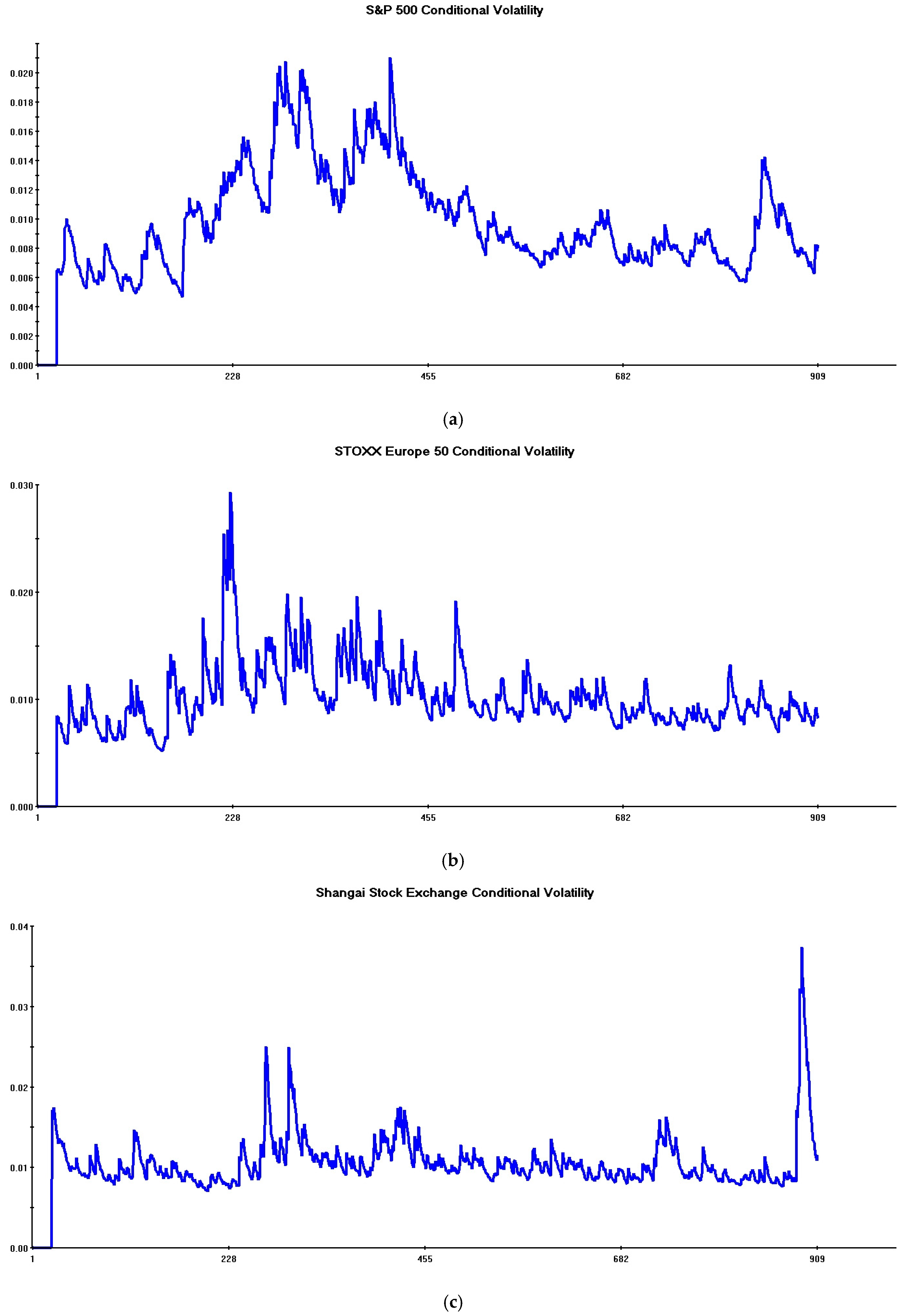
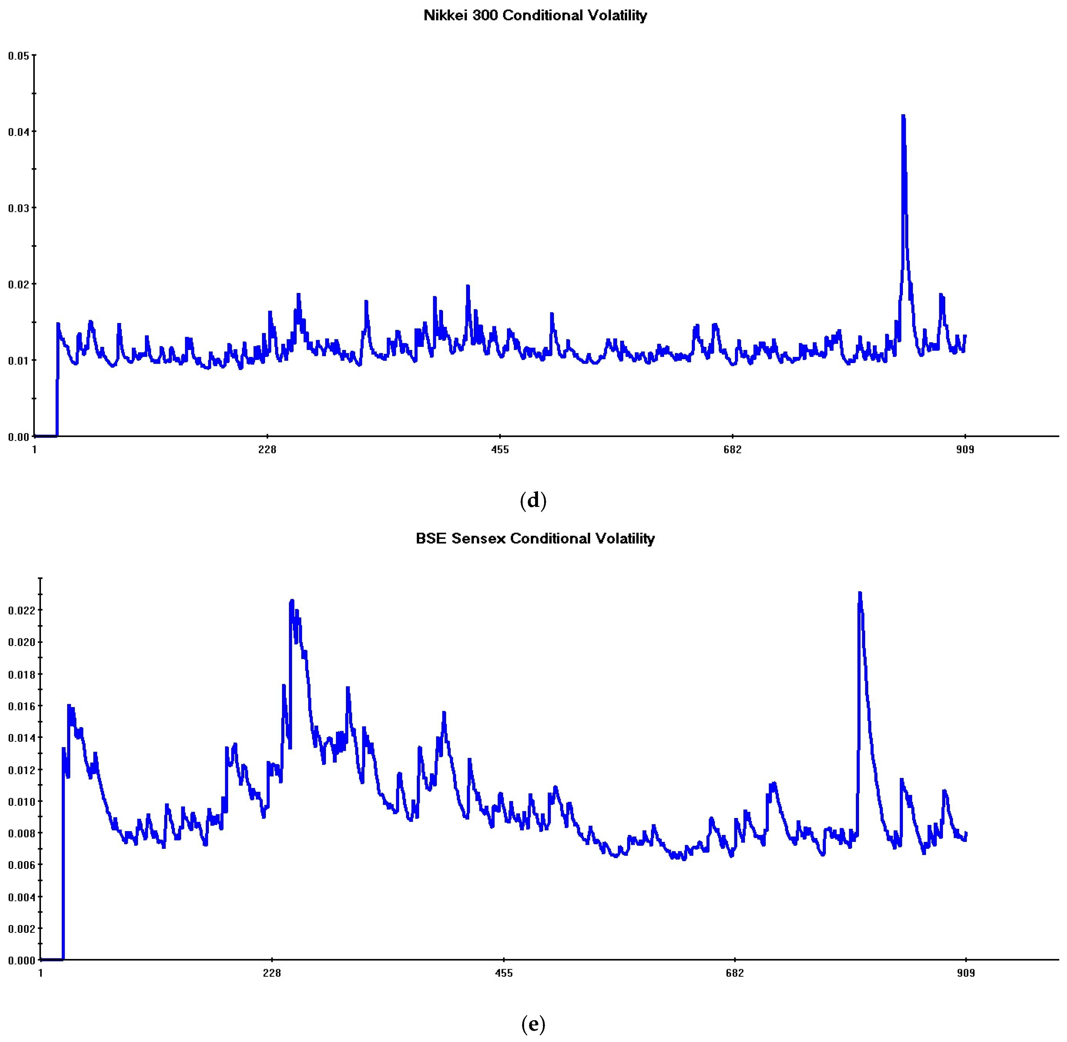
| 2 | Multivariate Garch models allow for obtaining consistent estimates of conditional volatility patterns. The Multivariate Garch model including only five global stocks represents the “benchmark” in the present paper, since all risk reductions obtained by incorporating additional defensive assets are evaluated against this “unhedged” portfolio. See Section 3 for technical details. Note finally that, although the sample begins on 29 March 2021, the starting date for volatility plots is 29 April 2021 since asset returns are expressed in log differences and twenty initial observations are lost to initialize the estimation process. |
| 3 | |
| 4 | While R. Engle (2002) DCC-Garch model can easily be applied to a large number of financial assets, the BEKK model suffers from the so-called “curse of dimensionality” problem (Bauwens et al., 2006), since its complexity grows exponentially with the number of assets. For this reason, the DCC-Garch model represents the natural choice in the context of the present empirical investigation. Turning to the ADCC model, its basic feature is the incorporation of an asymmetric response of volatility to negative and positive shocks. This approach is particularly powerful in empirical research focusing on optimal hedge ratios (see, e.g., Basher & Sadorsky, 2016), rather than to investigate the issue addressed in the present paper. |
| 5 | Throughout the paper, the risk-minimizing properties of hedged portfolios are analyzed assuming a VaR confidence level of 1%. The Maximum Expected Loss over a given time-horizon (one day in the case of this paper) is thus computed, focusing on the 1% tail of the returns distribution. A fixed risk-tolerance level of 99%, as in the present paper, represents the standard assumption in the applied financial literature and is consistent with current Basel guidelines confidence levels for banking supervision. Superior risk management practices, independent from ex ante subjective preferences of individual investors or risk management committees, have recently been put forward (see, e.g., Majumder, 2018). The improvement in VaR models allowing for endogenous time-variation of risk-tolerance levels is outside the scope of the present paper, although representing a suitable research direction for scenario-wise risk analysis. |
| 6 | Note that, under this alternative distributional assumption, R. Engle (2002) two-step original procedure is no longer applicable. The Maximum Likelihood estimator relies now on a more efficient approach, involving the simultaneous estimation of the model’s parameters and an additional degrees-of-freedom parameter relative to the multivariate t distribution (see Pesaran & Pesaran, 2010, Section 4 for technical details). The software used in this paper is Microfit 5.5 (see Pesaran & Pesaran, 2009). |
| 7 | Relevant exceptions, in this regard, are three hedged models, respectively incorporating Bitcoin, health stocks, and utilities stocks as defensive assets. Quantitative estimates of cross-correlation parameters suggest that conditional correlation structures are highly persistent, although in all cases conditional correlation processes are mean-reverting. |
| 8 | See Pesaran and Pesaran (2010), for a technical discussion on conditional evaluation procedures based on probability integral transforms. Under the null hypothesis of correct model specification, probability transforms estimates are serially uncorrelated and uniformly distributed in the interval (0, 1). |
| 9 | Parameters estimates are available from the author upon request. |
| 10 | One referee observed that the treatment of defensive weights scenarios is conceptually sound, but a clearer explanation of how portfolio weights are calculated would make the procedure more transparent. The approach followed in this paper to define asset weights for simulations relies on economic intuition and is therefore entirely ad hoc. This approach is, however, fully justified, given the purpose of this research. It may be useful to recall that, as regards bivariate portfolios, optimal asset allocation weights relying on Modern Portfolio Theory are often computed following Kroner and Sultan (1993) and Kroner and Ng (1998) seminal contributions (see, e.g., Tronzano (2022) for an empirical analysis inside bivariate portfolios including one global stock and one safe-haven asset (Gold or Swiss Franc)). Moving towards multiple asset frameworks, many alternative methodologies are available to compute optimal asset weights. A necessarily non-exhaustive list of these methodologies includes the following: Extensions of Markowitz (1952) classical mean-variance approach (although at the expense of greater model complexity); Hierarchical Risk Parity approaches to build asset clusters based on their correlation structures; Robust Optimization techniques to account for uncertainty in input parameters; Monte Carlo simulation to test portfolio performance under different conditions; and machine learning to identify complex patterns and relationships among asset returns. |
| 11 | It is interesting to observe that the main results obtained in this section are fully consistent with the Maximized Log-Likelihood statistics derived from models’ estimation. Intuitively, and allowing for the usual caveats related to outliers and model complexity, one would expect worse-performing VaR models to display lower log-likelihood values. A higher log-likelihood indicates that a specific model provides a better data fit, pointing out that estimated conditional variances and covariances are more consistent with the data. Therefore, from a risk management perspective, models displaying higher log-likelihoods are expected to deliver lower portfolio risks, since the asset allocation relying on these models has better risk-stabilizing properties. This is actually what happens in the present empirical investigation: the benchmark (unhedged) model exhibits the lowest log-likelihood (14,100); the single Bitcoin-hedged model provides a slightly higher value (15,849), whereas the single 5Y US note-hedged model reports the highest log-likelihood (17,584). Overall, these results provide further support for the robustness of our empirical evidence. A complete list of Maximized Log-Likelihood statistics is available upon request. |
| 12 | Therefore, if the portfolio includes five defensive assets, the total number of assets is ten (five defensive + five global stocks), and a weight of 0.10 is assigned to each of them. An analogous procedure holds to compute asset weights in the remaining cases (i.e., four, three, and two defensive assets). |
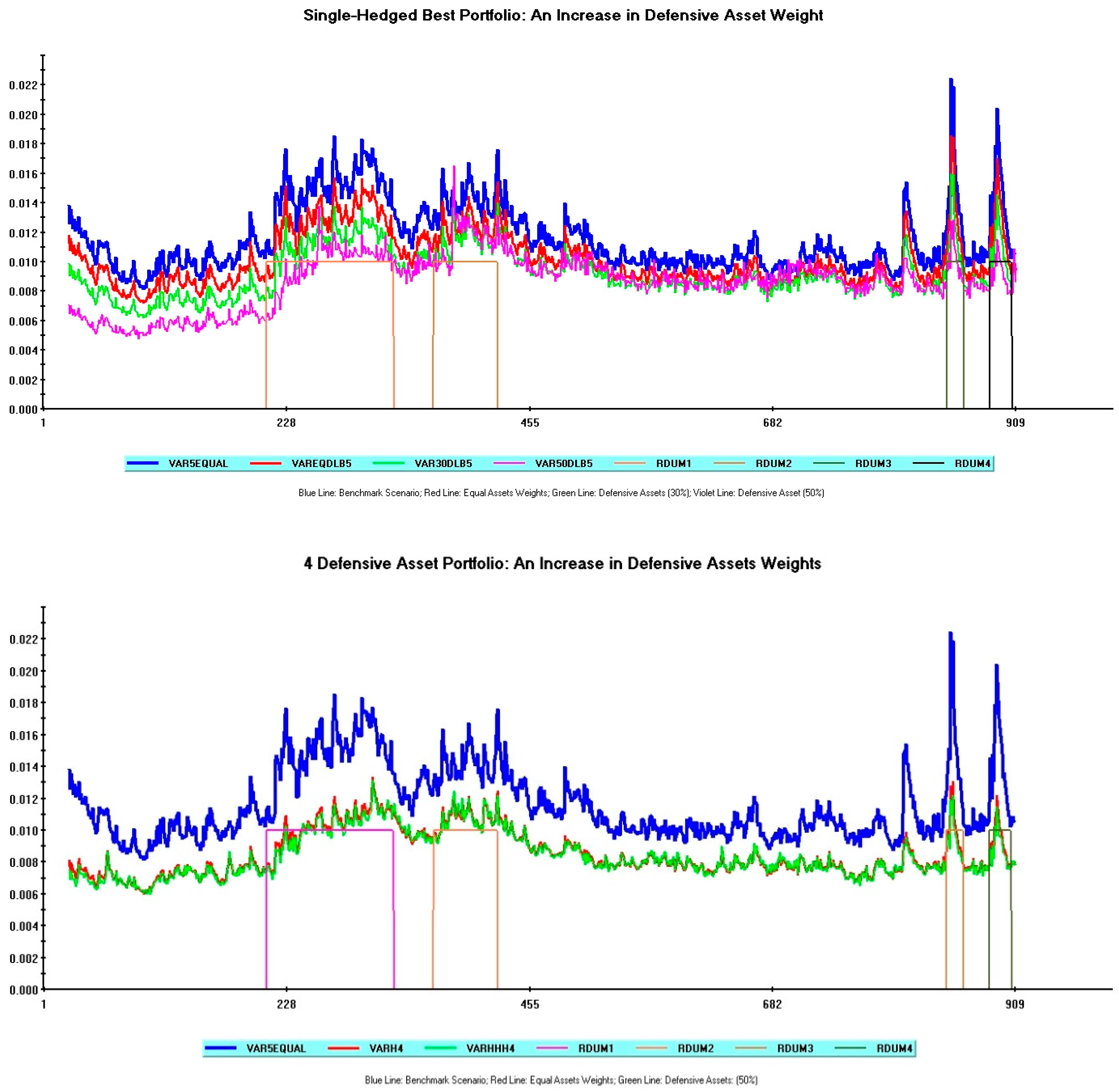
| 13 | Note that, as regards the 5-Defensive Asset portfolio, single portfolio weights are by construction identical in the “Equal Asset Weights” and in the “Moderately Defensive” scenarios. Average VaR values obtained in these two simulations are therefore identical. |
| 14 | In line with the previous section (see note 11), the VaR results for multiple-hedged portfolios are again fully in line with the Maximized Log-Likelihood values recorded from model estimates. The worse hedging properties recorded for less-diversified portfolios (Models 2A, 2B) are associated with lower log-likelihoods (Model 2A: 20,688; Model 2B: 20,381). The 4-Defensive Asset Model exhibiting the best risk-minimizing properties provides instead a much higher log-likelihood (26,349). Note, finally, that log-likelihood values for all multiple-hedged models are always higher than those of single-hedged models, thus reiterating the structural benefits of asset diversification. |
| 15 | In a more general perspective, moreover, the relatively small differences between average VaR values reported in Table 2 and Table 3 can be misleading if, as suggested by one referee, one reflects on the practical significance of these differences for investors by expressing them in terms of potential loss reduction. Let us suppose that a major international bank manages a portfolio of 50 million Euros on behalf of a high-net worth private client. Assume, as in the present paper, that this portfolio is invested in five global stocks. According to our results, if unhedged, this portfolio involves, during the selected sample period, a 1% probability of incurring a maximum loss amounting to 582,000 Euros (50,000,000 × 0.01164 = 582,000) each day. The corresponding maximum potential daily losses for a moderately defensive Bitcoin-hedged portfolio and a moderately defensive 4-Defensive assets portfolio amount, respectively, to 1,545,000 and 421,500 Euros. The potential loss reduction provided by the best-performing defensive portfolio (four defensive assets) is clearly substantial. This example shows that even relatively small VaR differences imply significant discrepancies in maximum potential losses, particularly if the empirical analysis relies on high-frequency data. For less wealthy investors, maximum potential losses are obviously smaller, but still significant. |
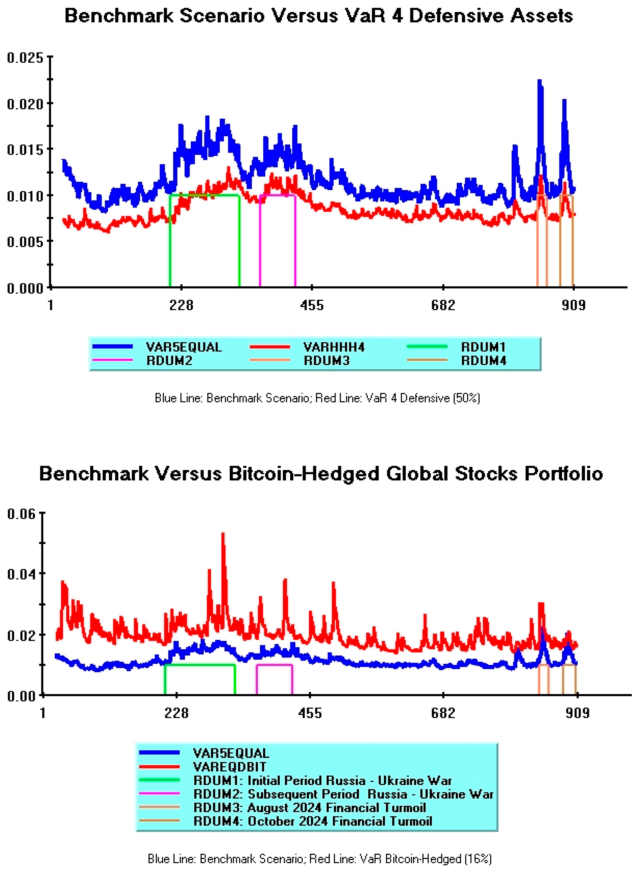
| 16 | One referee asked if this paper performed additional robustness checks, such as testing for alternative confidence levels (e.g., 95%), for VaR simulations. Systematic robustness checks of this kind were not performed, given the supportive empirical evidence obtained for model specification tests in Section 3.1 and the consistency documented between average VaR values and Likelihood Ratio statistics (see Section 3.1, note 11; Section 3.2, note 14). An occasional inspection of VaR simulations, allowing for alternative confidence levels, however, further confirmed the robustness of our results. Considering the benchmark (unhedged) scenario, and simulating dynamic VaRs with alternative confidence levels (i.e., 99% and 95%), the blue line corresponding to the stricter tolerance level (1%) is consistently higher than the red line corresponding to the looser tolerance level (5%). This is in line with a priori expectations, since the former case (blue line: tolerance level 1%) focuses on the fraction of expected returns corresponding to the worst portfolio losses. |
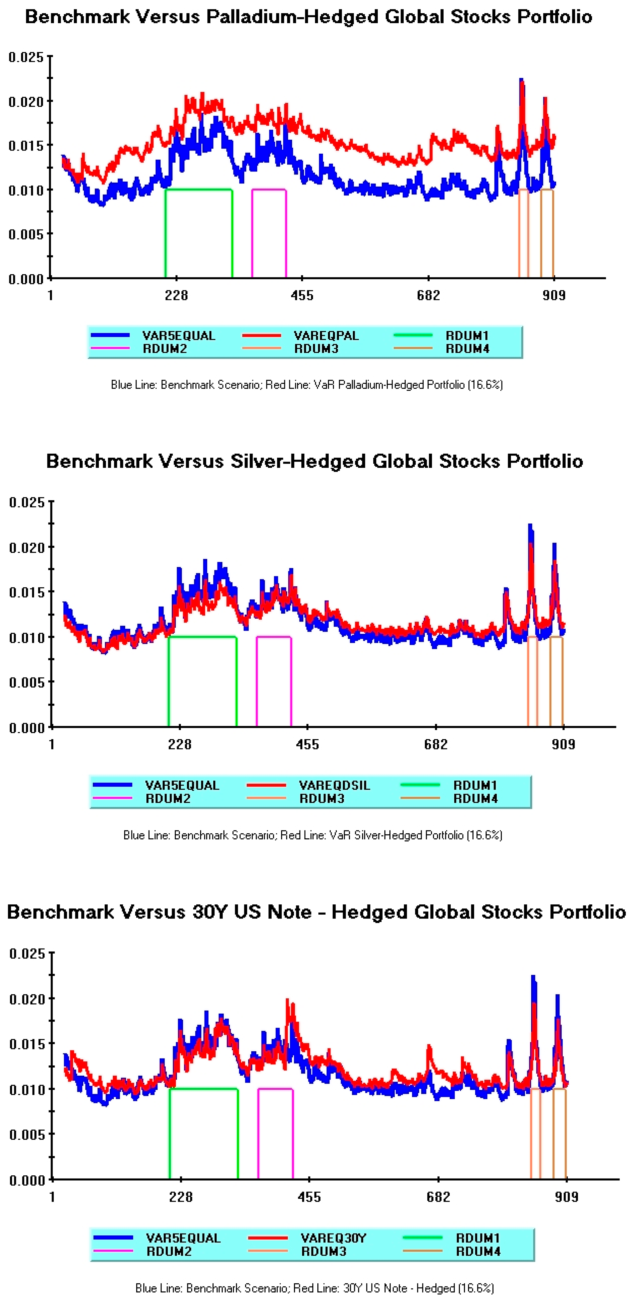
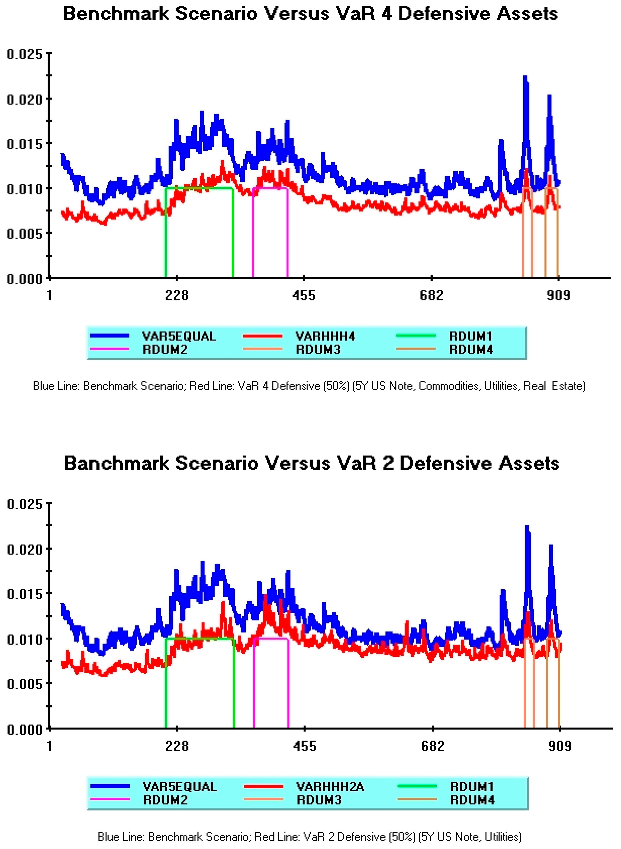
| 17 | The benchmark scenario pattern is obviously the same in both plots, although its shape in Figure 2 appears different due to the different scales reproduced on the vertical axes. |
| 18 | Note, however, that the average VaR difference between these multiple-hedged portfolios is low, as witnessed by their average VaR values appearing in Table 3. |
| 19 | |
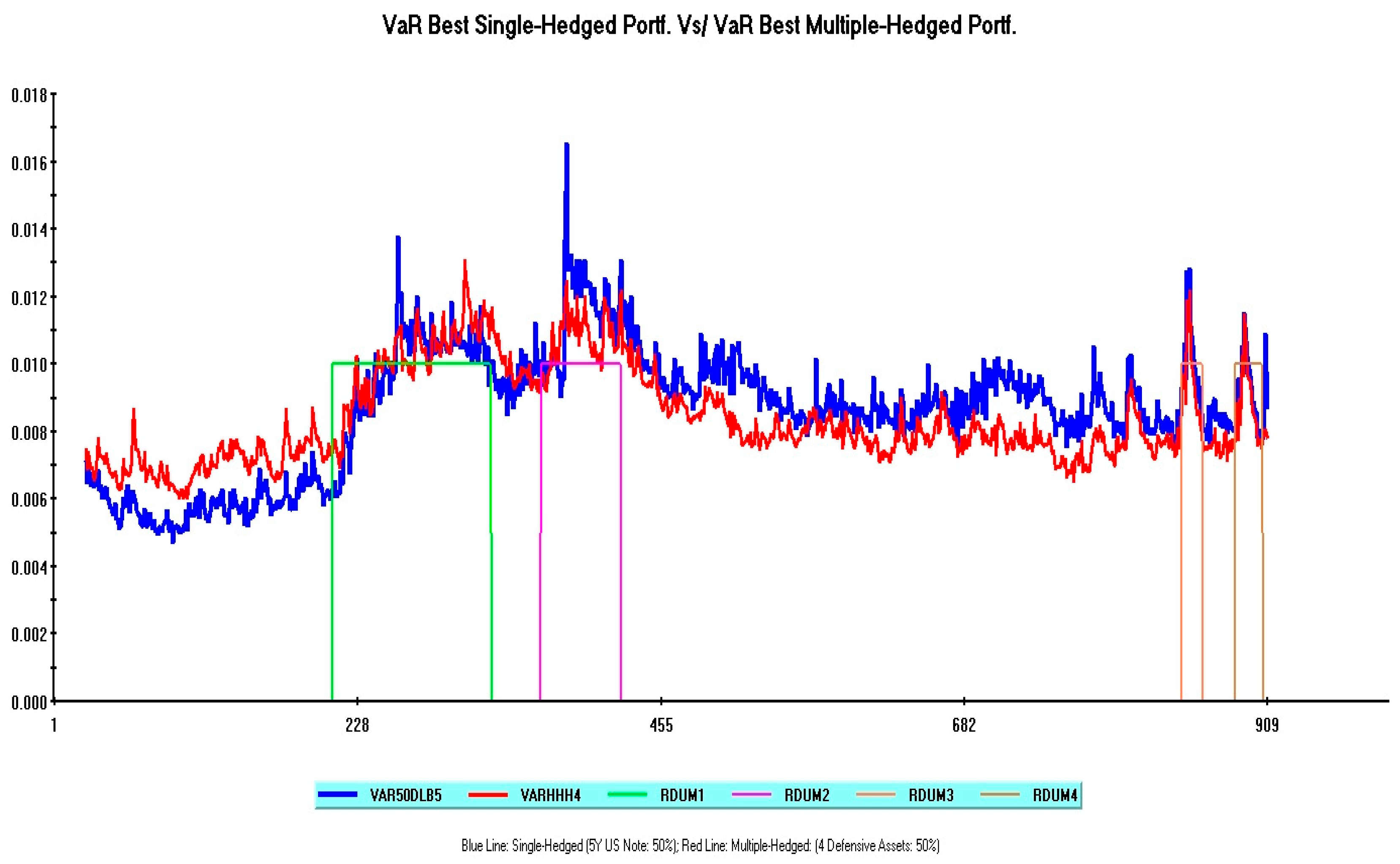
| 20 | The standard deviation of VaR values associated with the multiple-hedged portfolio is 0.0014, a value which favorably compares with that provided by the single-hedged portfolio (0.00184). |
References
- Abdul Aziz, N. S., Vrontos, S., & Hasim, H. M. (2019). Evaluation of multivariate Garch models in an optimal asset allocation framework. North American Journal of Economics and Finance, 47(1), 568–596. [Google Scholar] [CrossRef]
- Basher, S. A., & Sadorsky, P. (2016). Hedging emerging market stock prices with oil, gold, VIX, and bonds: A comparison between DCC, ADCC and GO-GARCH. Energy Economics, 54(C), 235–247. [Google Scholar] [CrossRef]
- Baur, D. G., Hong, K. H., & Lee, A. D. (2018). Bitcoin: Medium of exchange or speculative asset? Journal of International Financial Markets, Institutions and Money, 54(5), 177–189. [Google Scholar] [CrossRef]
- Baur, D. G., & Lucey, B. M. (2010). Is gold a hedge or a safe haven? An analysis of stocks, bonds and gold. Financial Review, 45(2), 217–229. [Google Scholar] [CrossRef]
- Baur, D. G., & McDermott, T. K. (2010). Is gold a safe haven? International evidence. Journal of Banking and Finance, 34(8), 1886–1898. [Google Scholar] [CrossRef]
- Bauwens, L., Laurent, S., & Rombouts, J. V. K. (2006). Multivariate GARCH models: A survey. Journal of Applied Econometrics, 21(1), 79–109. [Google Scholar] [CrossRef]
- Belhassine, O., & Riahi, M. (2025). Searching for safe haven assets against American and European stocks during the Russo-Ukrainian war. Studies in Economics and Finance, 42(2), 352–372. [Google Scholar] [CrossRef]
- Boubaker, S., Goodell, J. W., Pandey, D. K., & Kumari, V. (2022). Heterogeneous impact of wars on global equity markets: Evidence from the invasion of Ukraine. Finance Research Letters, 48(3), 102934. [Google Scholar] [CrossRef]
- Cappiello, L., Engle, R. F., & Sheppard, K. (2006). Asymmetric dynamics in the correlations of global equity and bond returns. Journal of Financial Econometrics, 4(4), 537–572. [Google Scholar] [CrossRef]
- Engle, R. (2002). Dynamic conditional correlation: A simple class of multivariate generalized autoregressive conditional heteroscedasticity models. Journal of Business & Economic Statistics, 20(3), 339–350. [Google Scholar]
- Engle, R. F., & Kroner, K. F. (1995). Multivariate simultaneous generalized ARCH. Econometric Theory, 11(1), 122–150. [Google Scholar] [CrossRef]
- Fakhfekh, M., Manzli, Y., Jeribi, A., & Bejaoui, A. (2023). Can cryptocurrencies be a safe-haven during the 2022 Ukraine crisis? Implications for G7 investors. Global Business Review. [Google Scholar] [CrossRef]
- Ghorbali, B., Kaabia, O., Naoui, K., & Urom, C. (2023). Wheat as a hedge and safe haven for equity investors during the Russia-Ukraine war. Finance Research Letters, 58(C), 104534. [Google Scholar] [CrossRef]
- Guoli, M., Weiguo, Z., Chunzhi, T., & Xing, L. (2022). Predicting the portfolio risk of high-dimensional international stock indices with dynamic spatial dependence. North American Journal of Economics and Finance, 59(C), 101570. [Google Scholar]
- Hachicha, N., Amar, A. B., Slimane, B. I., Bellalah, M., & Prigent, J. (2022). Dynamic connectedness and optimal hedging strategy among commodities and financial indices. International Review of Financial Analysis, 83(3), 102290. [Google Scholar] [CrossRef]
- Hanif, W., Andraz, J. M., Gubareva, M., & Teplova, T. (2024). Are REITS hedge or safe haven against oil price falls? International Review of Economics and Finance, 89(PA), 1–16. [Google Scholar] [CrossRef]
- Jarque, C. M., & Bera, A. K. (1980). Efficient tests for normality, homoscedasticity and serial independence of regression residuals. Economics Letters, 6(3), 255–259. [Google Scholar] [CrossRef]
- Khan, M. N. (2025). Assessing the impact of geopolitical crises on global financial markets: Insights from the novel TVP-VAR model. Journal of Economic Integration, 40(1), 29–52. [Google Scholar] [CrossRef]
- Kimball, M. S. (1990). Precautionary saving in the small and in the large. Econometrica, 58(1), 53–73. [Google Scholar] [CrossRef]
- Kroner, K. F., & Ng, V. K. (1998). Modeling asymmetric comovements of asset returns. Review of Financial Studies, 11(4), 817–844. [Google Scholar] [CrossRef]
- Kroner, K. F., & Sultan, J. (1993). Time dynamic varying distributions and dynamic hedging with foreign currency futures. Journal of Financial and Quantitative Analysis, 28(4), 535–551. [Google Scholar] [CrossRef]
- Majumder, D. (2018). Value-at-Risk based on time-varying risk tolerance level. Theoretical Economic Letters, 8(1), 111–118. [Google Scholar] [CrossRef]
- Markowitz, H. (1952). Portfolio selection. Journal of Finance, 7(1), 77–91. [Google Scholar]
- Naifar, N. (2025). Navigating risk in crypto markets: Connectedness and strategic allocation. Risks, 13(8), 141. [Google Scholar] [CrossRef]
- Pesaran, B., & Pesaran, M. H. (2009). Time series econometrics using microfit 5.0: A user’s manual. Oxford University Press. [Google Scholar]
- Pesaran, B., & Pesaran, M. H. (2010). Conditional volatility and correlations of weekly returns and the VaR analysis of 2008 stock market crash. Economic Modelling, 27(6), 1398–1416. [Google Scholar] [CrossRef]
- Pivrnec, T. (2024). Performance and risk profiles of stocks and cryptocurrencies during the Russian invasion of Ukraine [Master’s thesis, Charles University, Faculty of Social Sciences, Institute of Economic Studies]. [Google Scholar]
- Prayut, J., & Sashi, J. (2019). Can machine learning based portfolios outperform traditional risk-based portfolios? The need to account for covariance misspecification (mimeo). Indian Institute of Science. [Google Scholar]
- Sears, S., & Wei, K. C. (1985). Asset pricing, higher moments and the market risk premium: A note. Journal of Finance, 40(4), 1251–1253. [Google Scholar] [CrossRef]
- Shaik, M., Jamil, S. A., Hawaldar, I. T., Sahabuddin, M., Rabbani, M. R., & Atif, M. (2023). Impact of geo-political risk on stocks, oil, and gold returns during GFC, COVID-19, and Russian-Ukraine war. Cogent Economics & Finance, 11(1), 2190213. [Google Scholar]
- Thi Thuy, V. L., Kim Oanh, T., & Hong Ha, N. T. (2024). The roles of gold, US dollar, and bitcoin as safe-haven assets in times of crisis. Cogent Economics & Finance, 12(1), 2322876. [Google Scholar] [CrossRef]
- Tronzano, M. (2022). Optimal portfolio allocation between global stock indexes and safe haven assets: Gold versus the Swiss Franc (1999–2021). Journal of Risk and Financial Management, 15(6), 241. [Google Scholar] [CrossRef]
- Ullah, M., Sohag, K., Doroshenko, S., & Mariev, O. (2024). Examination of bitcoin hedging, diversification and safe-haven ability during financial crisis: Evidence from equity, bonds, precious metals and exchange rate markets. Computational Economics, 66(1), 835–867. [Google Scholar] [CrossRef]
- Yousaf, I., Patel, R., & Yarovaya, L. (2022). The reaction of G20+ stock markets to the Russia-Ukraine conflict “black swan” event: Evidence from event study approach. Journal of Behavioral and Experimental Finance, 35(1), 100723. [Google Scholar] [CrossRef]
- Zhu, Y., Taasim, S. I., & Daud, A. (2025). Volatility modeling and tail risk estimation of financial assets: Evidence from gold, oil, bitcoin, and stocks of selected markets. Risks, 13(7), 138. [Google Scholar] [CrossRef]
| (A) | |||||||||
| DUS | DEU | DCH | DJP | DIN | |||||
| Mean | 0.0004 | 0.0001 | −0.0001 | −0.00002 | 0.0003 | ||||
| Stand. Dev. | 0.010 | 0.010 | 0.011 | 0.012 | 0.010 | ||||
| Skewness | −0.245 | −0.131 | 0.012 | −0.448 | −0.609 | ||||
| Excess Kurtosis | 1.937 | 3.410 | 5.688 | 6.436 | 4.340 | ||||
| Jarque–Bera | 151.1 *** | 442.5 *** | 1224.2 *** | 1597.6 *** | 769.0 *** | ||||
| ARCH (1) | 13.0 *** | 35.7 *** | 52.9 *** | 159.7 *** | 62.3 *** | ||||
| ARCH (6) | 80.7 *** | 84.2 *** | 193.9 *** | 178.9 *** | 79.2 *** | ||||
| Ljung–Box (1) | 0.301 | 0.182 | 0.297 | 12.65 *** | 0.373 | ||||
| Ljung–Box (6) | 2.895 | 3.522 | 5.897 | 21.20 *** | 3.776 | ||||
| (B) | |||||||||
| DLHEA | DLUTI | DLRE | DSIL | DPAL | DLCOM | DLB5 | DLB30 | DBIT | |
| Mean | 0.0001 | 0.0001 | −0.0002 | 0.0003 | −0.0009 | 0.0001 | 0.0000 | 0.0000 | 0.0002 |
| Stand. Dev. | 0.009 | 0.008 | 0.010 | 0.017 | 0.028 | 0.010 | 0.005 | 0.016 | 0.037 |
| Skewness | −0.415 | −0.305 | 0.065 | 0.037 | 0.099 | −0.510 | 1.534 | 3.054 | −0.466 |
| Excess Kurtosis | 1.889 | 1.759 | 1.951 | 1.296 | 2.267 | 2.442 | 15.01 | 32.80 | 4.429 |
| Jarque–Bera | 161.1 *** | 131.2 *** | 144.6 *** | 63.7 *** | 195.9 *** | 265.1 *** | 8889.1 *** | 42,116.4 *** | 775.2 *** |
| ARCH (1) | 6.39 ** | 13.6 *** | 6.18 ** | 0.71 | 3.97 ** | 3.08 * | 0.29 | 0.05 | 1.61 |
| ARCH (6) | 43.9 *** | 39.2 *** | 11.1 * | 7.7 | 5.70 | 114.7 *** | 0.62 | 0.73 | 14.8 ** |
| Ljung–Box (1) | 4.326 ** | 10.58 *** | 0.018 | 0.553 | 1.564 | 5.975 ** | 12.58 *** | 0.887 | 0.328 |
| Ljung–Box (6) | 5.203 * | 17.09 *** | 3.746 | 2.874 | 5.821 | 12.55 * | 19.78 *** | 3.286 | 4.585 |
| 5 Global Stocks (Benchmark) | Bitcoin Hedged | Palladium Hedged | Silver Hedged | 30Y US Note Hedged | Health Hedged | Commod. Index Hedged | Utilities Hedged | Real Estate Hedged | 5Y US Note Hedged | |
|---|---|---|---|---|---|---|---|---|---|---|
| Equal Asset Weights (16.6%) | 0.01164 | 0.0199 | 0.0153 | 0.0116 | 0.0121 | 0.0112 | 0.0106 | 0.01064 | 0.0103 | 0.0102 |
| Moderately Defensive Scenario Safe Haven (30%) | - | 0.0309 | 0.0223 | 0.0143 | 0.0148 | 0.0117 | 0.0111 | 0.0106 | 0.0106 | 0.0092 |
| Strongly Defensive Scenario Safe Haven (50%) | - | 0.0487 | 0.0346 | 0.0205 | 0.0210 | 0.0136 | 0.0137 | 0.0119 | 0.0130 | 0.0086 |
| Benchmark Unhedged Stock Portfolio | 5 Defensive Assets | 4 Defensive Assets | 3 Defensive Assets | 2A Defensive Assets | 2B Defensive Assets | |
|---|---|---|---|---|---|---|
| Equal Asset Weights | 0.01164 | 0.00868 | 0.00851 | 0.00878 | 0.00951 | 0.00920 |
| Moderately Defensive Scenario Safe Haven (50%) | - | 0.00868 | 0.00843 | 0.00847 | 0.00884 | 0.00884 |
| Strongly Defensive Scenario Safe-Haven (60%) | - | 0.00870 | 0.00849 | 0.00857 | 0.00894 | 0.00924 |
Disclaimer/Publisher’s Note: The statements, opinions and data contained in all publications are solely those of the individual author(s) and contributor(s) and not of MDPI and/or the editor(s). MDPI and/or the editor(s) disclaim responsibility for any injury to people or property resulting from any ideas, methods, instructions or products referred to in the content. |
© 2025 by the author. Licensee MDPI, Basel, Switzerland. This article is an open access article distributed under the terms and conditions of the Creative Commons Attribution (CC BY) license (https://creativecommons.org/licenses/by/4.0/).
Share and Cite
Tronzano, M. Assessing the Effectiveness of Some Defensive Assets in Global Stock Portfolios: Evidence from Daily Data (2021–2024). J. Risk Financial Manag. 2025, 18, 704. https://doi.org/10.3390/jrfm18120704
Tronzano M. Assessing the Effectiveness of Some Defensive Assets in Global Stock Portfolios: Evidence from Daily Data (2021–2024). Journal of Risk and Financial Management. 2025; 18(12):704. https://doi.org/10.3390/jrfm18120704
Chicago/Turabian StyleTronzano, Marco. 2025. "Assessing the Effectiveness of Some Defensive Assets in Global Stock Portfolios: Evidence from Daily Data (2021–2024)" Journal of Risk and Financial Management 18, no. 12: 704. https://doi.org/10.3390/jrfm18120704
APA StyleTronzano, M. (2025). Assessing the Effectiveness of Some Defensive Assets in Global Stock Portfolios: Evidence from Daily Data (2021–2024). Journal of Risk and Financial Management, 18(12), 704. https://doi.org/10.3390/jrfm18120704


