Diffusion on the Peer-to-Peer Network

Abstract

In a peer-to-peer complex environment, information is permanently diffused. Such an environment can be modeled as a graph, where there are flows of information. The interest of such modeling is that (1) one can describe the exchanges through time from an initial state of the network, (2) the description can be used through the fit of a real-world case and to perform further forecasts, and (3) it can be used to trace information through time. In this paper, we review the methodology for describing diffusion processes on a network in the context of exchange of information in a crypto (Bitcoin) peer-to-peer network. Necessary definitions are posed, and the diffusion equation is derived by considering two different types of Laplacian operators. Equilibrium conditions are discussed, and analytical solutions are derived, particularly in the context of a directed graph, which constitutes the main innovation of this paper. Further innovations follow as the inclusion of boundary conditions, as well as the implementation of delay in the diffusion equation, followed by a discussion when doing approximations useful for the implementation. Numerous numerical simulations additionally illustrate the theory developed all along the paper. Specifically, we validated, through simple examples, the derived analytic solutions, and implemented them in more sophisticated graphs, e.g., the ring graph, particularly important in crypto peer-to-peer networks. As a conclusion for this article, we further developed a theory useful for fitting purposes in order to gain more information on its diffusivity, and through a modeling which the scientific community is aware of.

1. Introduction

This document aims at describing the diffusion of information in the peer-to-peer (P2P) network related to a crypto, for instance Bitcoin, through a fundamental diffusion approach. The information could be anything, but the object of communication between agents (i.e., miners and users), and, to add context, it could be the hash calculation. This designates the processes which calculate hashes for mining blocks, given relevant remaining transactions to hash. More specifically, miners have the purpose of hash transactions within a list of transactions—the memory pool—which appear in the next block in the blockchain Lipton and Treccani (2021). Each transaction circulates from node to node in the memory pool used for remembering all new transactions, and miners receiving new transaction lists, supposing no double spending, start to generate hashes to create the new block. To this extent, the hash calculation starts as long as miners receive the list of transactions, thus the hash calculation can be seen as the information of transactions diffusing along the network (see Shahsavari et al. (2017) for a more theoretical discussion). The more a miner receives transactions to be mined, the more he/she is likely to calculate hashes, i.e., the stronger the hash calculation. On the contrary, if there is a low amount of information, i.e., not so many transactions to hash, then the lower the amount of transactions are to be hashed, and the lower the hash calculation. Conversely, if the hash calculation is high, this means that the miner has likely received a long list of transactions ready to be hashed. The hash calculation is intimately linked to the hash rate, so we will name this type of diffusion: diffusion of hash rate. In another more economical context, the diffused information could simply be Bitcoin cash flows.

This is true only if all miners have equal power of computing hashes, which we know is not realistic. This is not an issue: the diffusion model should depend on each node, and we will need to incorporate a rate of creation of hashes to assign to each node. In essence, not only do we have a diffusion of hash rate, but also the creation of hashes, increasing the hash rate for each miner. Being able to derive the hash rate with respect to time and node is being able to predict such an evolution for all nodes, at a given time and context, which is one main motivation for this approach.

A simple but fundamental physics model of diffusion is given by the famous diffusion equation,

$$\frac{\partial h}{\partial t}=D\Delta h+\mathsf{\Gamma },$$

(1)

where h is the hash rate (or more generally, a ‘rate’ of information), t is the time variable, D is the diffusion coefficient throughout the network, and $\mathsf{\Gamma }$ is the local hash creation rate. The operator $\Delta$ is called the Laplacian operator. One may think we could handle this approach and solve the equation for h. However, what do spatial coordinates represent? It seems that the majority of physics fields where this equation applies contains spatial coordinates, which are real numbers with respect to a pre-defined coordinate system. This is not the case for a proper network.

This means we need to handle the diffusion theory on a graph. There have already been established approaches somehow related to the diffusion description on a graph, with many applications (e.g., Bondy and Murty 2007; Pacreau et al. 2021; Thanou et al. 2017; Viriyasitavat and Hoonsopon 2019). We discuss some of the approaches for modeling diffusion on a network.

The paper An et al. (2021) specifies an optimality approach for minimizing the maximum regret due to decision taken in an uncertainty environment, and specifically calculates the maximal regret through a linear program. This program has the advantage of considering the connectivity of the network, and the evolution of the information diffusion should be a relevant complement to describe the structure of the network. The paper Mikhaylov (2021) defends Hayek’s theory of private money, which, once applied to a state, should avoid a significant amount of private money within the population of this state and reduce the inequalities by means of further regulations through central banks digital currencies (CBDC). This imposes a certain structure in the network of exchanges: the current Bitcoin P2P network is distributed, and the application of this theory would make it change into a more centralized network. The diffusion properties may significantly change from one type to the other (see Section 7 for numerical illustrations), and our approach applies to both different types. The authors in the paper Hollanders et al. (2014) model a P2P network as a bipartite graph, where one family is the set of files, and the other is the set of peers. This way of modeling allows to find an ‘S’ shape in the dynamic of the information diffusion, and such a shape is a strong expectation of the social networks community. The equations guiding the evolution are through the susceptible/infectious (SI) equations. There are underlying assumptions, such as the strong one: the constancy of population. The paper Manini and Gribaudo (2008) engages a probabilistic approach of diffusion of files into a P2P network. In Musa et al. (2018), the diffusion methodologies applied to a P2P network are explicitly reviewed. If not based on the SI approach, the models are essentially probabilistic. Finally, the authors in Li et al. (2019) see the blockchain as a kind of Markov chain.

Interestingly, all the mentioned approaches overall focus on probabilistic modeling for the diffusion processes on a graph. This present study proposes to focus on the more fundamental aspects of the diffusion behavior, mainly governed by an equation of the style of Equation (1). It is worth stressing that the operator $\mathsf{\Gamma }$ is very general, and can be the source of randomness through, for instance, non-linearities, bringing chaos into the system. However, one possibly can also include probability in $\mathsf{\Gamma }$, which would make the present study very general. More conceptually, $\mathsf{\Gamma }$ can gather any network specificity, such as its consensus, since it is related to sources of information.

However, some definitions already introduced in some of the previous studies, and including the Laplacian operator, may need to be further discussed, especially from a more intuitive and fundamental view of sharing information between two vertices of a graph. This is especially true when the graph is directed. Thus, in the context of diffusion on a P2P network, we need, for deriving the appropriate diffusion equation, to introduce the derivative and the integration on a graph, for a function f defined on each node x at a given time t. The Laplacian operator will follow. One understands that deriving the appropriate diffusion equation is a task in itself. Then, once derived, we need to solve the equation, which represents another task. In addition, we will see that there are different possible Laplacian operators for a diffusion theory (at least two), and we will focus on them separately. We will need some linear algebra tools to do it, as a graph is equivalent to its adjacency matrix, and, conversely, any matrix gives a (weighted) graph.

We now discuss the two hypotheses made (and mitigated) in this study. The first one is that graphs are undirectional. This is a strong assumption, as it means that once a vertex agent receives information that it did not previously have, then it will give back part of it to the source. Although this might be convenient in the context of bitcoin exchange (Alice sends some bitcoins to Bob, but also to herself, i.e., she generates new addresses she owns to send part of the total amount of bitcoins), a piece of information, whatever its type, has no reason to come back to its source. Considering that a directed graph is essential if we need to describe the interactions within a P2P network, this is what we do in this paper, and this constitutes the main innovation of the present study.

Another hypothesis is made in this modeling: when a vertex agent receives a piece of information, he/she immediately treats it and diffuses it to its neighbors. In other words, the response to the information reception is immediate. This is also a strong assumption, as, for instance, cash flows are performed in a delayed manner. Thus, Alice sends some bitcoins to Bob, but Bob does not immediately send a part (or more) of it to Charlie. In fact, the immediate response is the straightforward consequence of the structure of the diffusion equation, whose solutions are a differentiable function of time. It turns out that one way to make a non-differentiable solution at some given times is to introduce time dependency in the Laplacian operator, and the Heaviside function (whose value is 0 below a given time, and 1 above it) is a relevant candidate for differentiability breaking at selected points in time. Introducing Heaviside functions in the Laplacian operator is a much easier task in the context of graph modeling, for the reason that there are no discontinuity issues for the variable x, usually continuous, and here being discrete (and representing the node index). We engage this point of view at the end of the study.

The rest of this paper is depicted as follows. Section 2 is an introduction to the modeling, with many fundamental definitions which will imply the Laplacian ones, as well as the diffusion theory. Section 3 derives and solves the diffusion equation defined on an undirected graph. It is worth pointing out that the two previous sections are strongly inspired from Chung et al. (2007). The rest of this paper constitutes the main innovations. Section 4 introduces two different types of equilibrium notion, the standard one ($t\to \infty$) and the blockchain one ($t=10$ min for Bitcoin), as well as some conceptual links between both. Section 5 shows the implementation of the derived solution in Section 3. 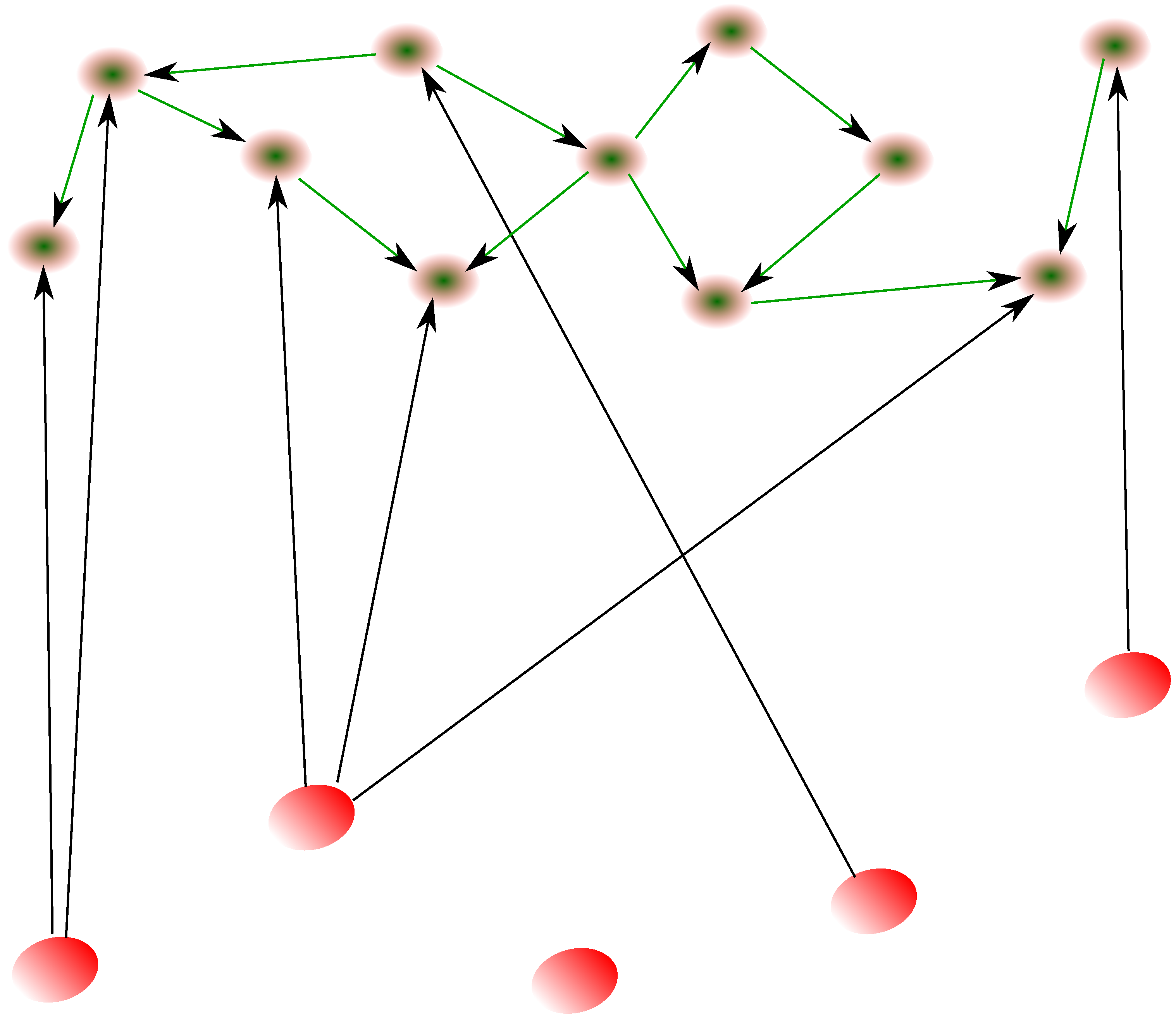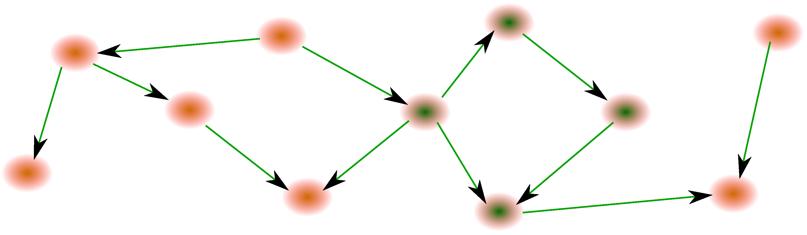Section 6 is an important generalization of the approach done thus far: it introduces the diffusion equation and its resolution in a directed graph, very important properties of the P2P network as already discussed above. 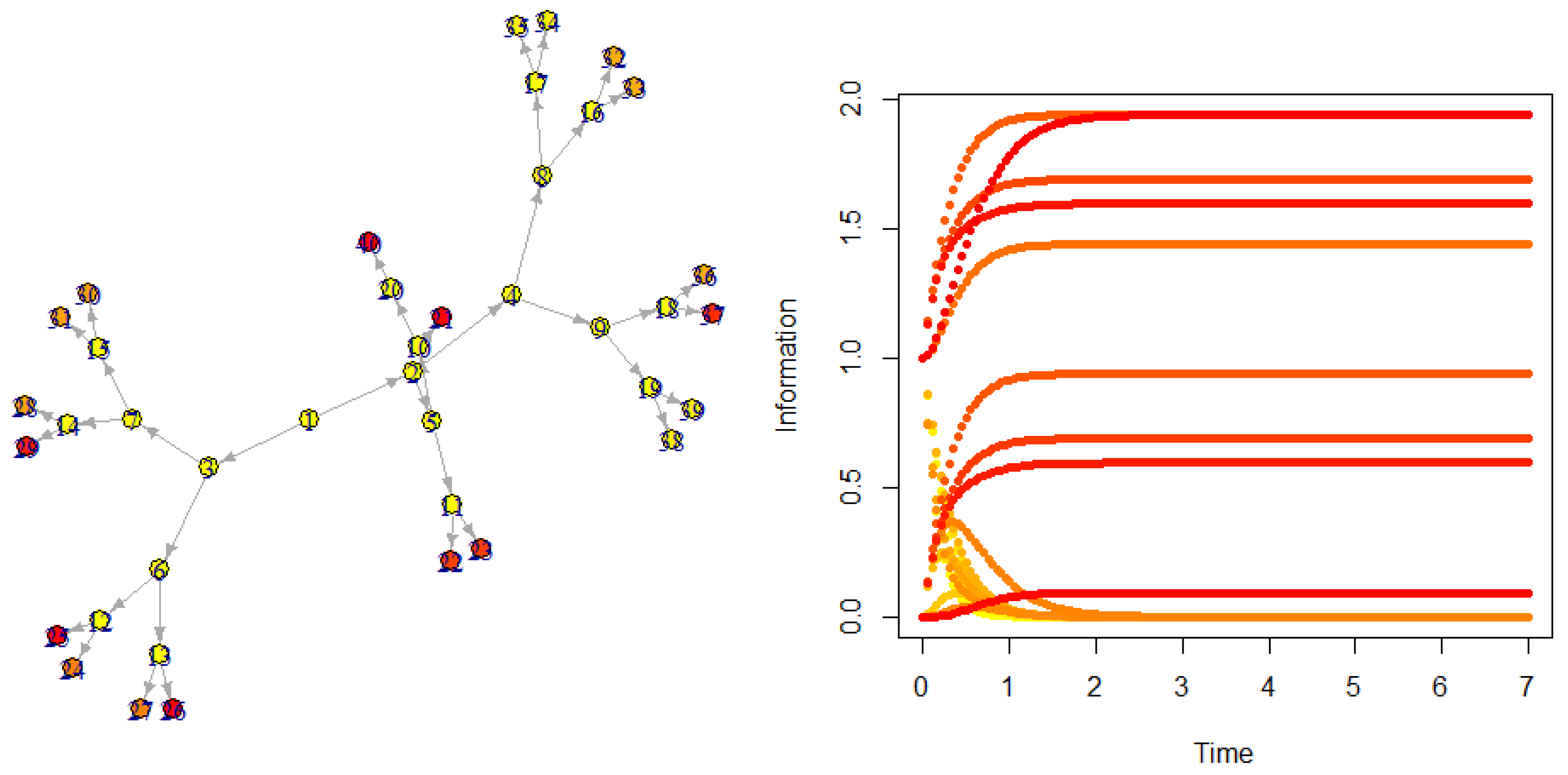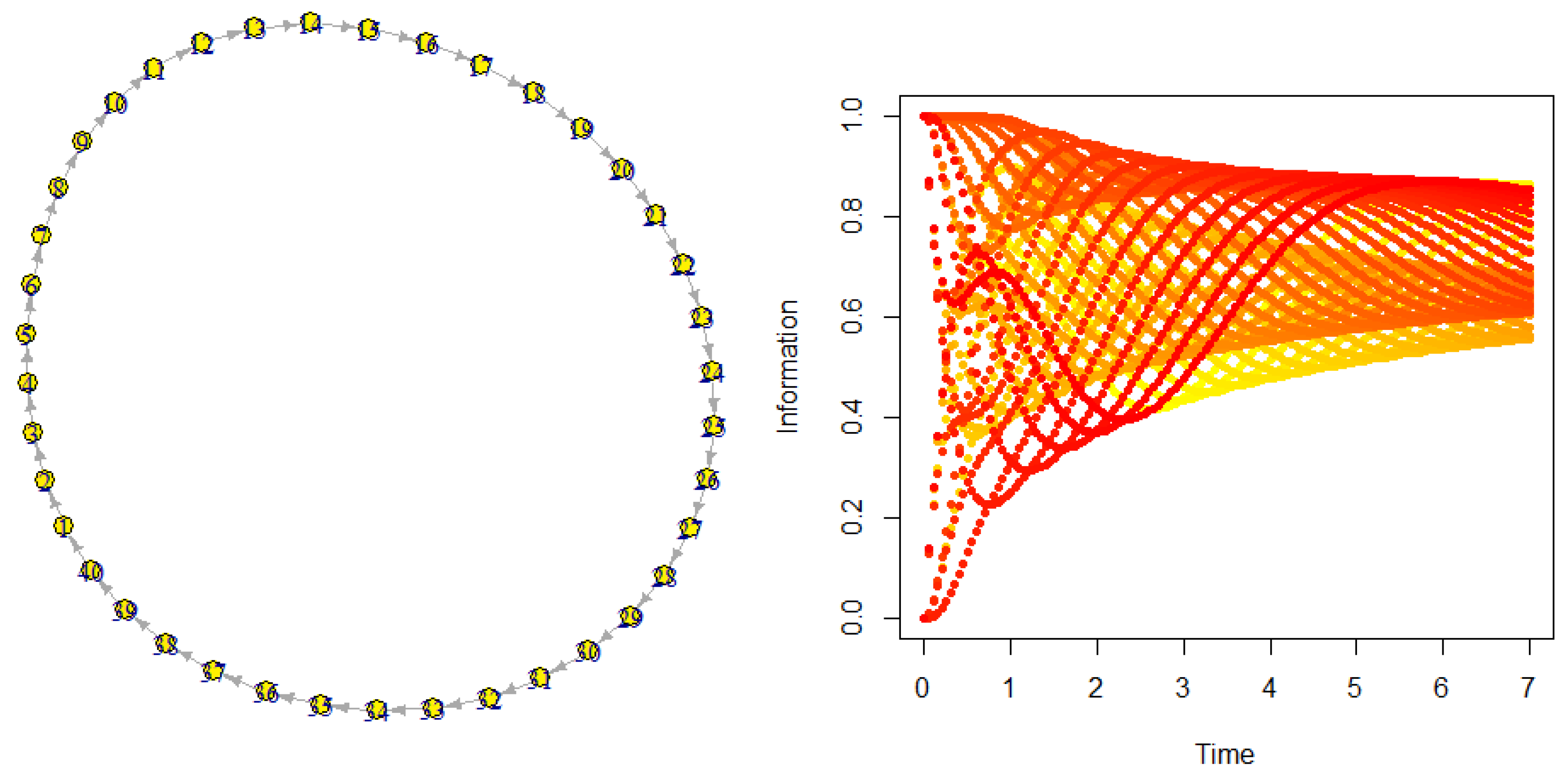Section 7 shows numerical illustrations of the previous section for several famous networks (including the Erdos–Reyni network, or the binary tree). Section 8 is the direct implication of the previous directed graph case when there are boundary conditions, typically certain vertices constantly sending information to the rest of the network. Finally, Section 9 includes delay in the response of nodes when they receive information. The last section concludes the study.

2. Modelling the P2P Network

2.1. Introduction to Graph Theory

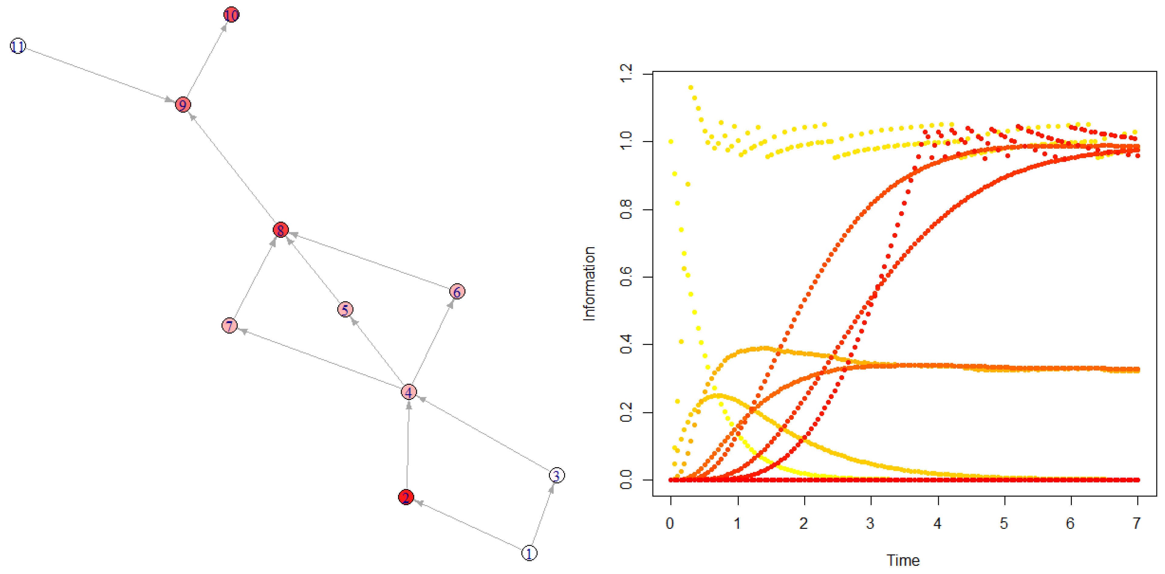
Let $G=(E,V)$ be a graph, that is a set of nodes E and a set of hedges V, composed of pairs of nodes in E. Thus, if $x\in V$, i.e., x is a node of G, and $y\in E$ is another node of G; if $(x,y)\in V$, we say that the nodes x and y are connected in G. We suppose that G is connected (that is, there exists a connection between any two nodes of G), unoriented (x to y or y to x is the same) and unweighted (all the paths are equally effective); this last hypothesis may be relaxed in the future. An example of such a graph is shown in Figure 1.

Figure 1. Illustration of a graph. The balls are nodes, which are connected by edges, the segments. Here, nodes have between one and four neighbors. In particular, node 6 diffuses information (e.g., list of transactions) to its neighbors, i.e., nodes 3, 5, and 7.

There is a matrix equivalence for such a graph. Node 1 is connected to nodes 2 and 3, in Figure 1, but not to any other node. We can represent the graph G by a matrix A, which is named the adjacency matrix. If we arbitrarily label nodes with numbers, the adjacency matrix for the graph G in Figure 1 is given by

$$A=\left(\begin{array}{ccccccccc}0& 1& 1& 0& 0& 0& 0& 0& 0\\ 1& 0& 1& 0& 0& 0& 0& 0& 0\\ 1& 1& 0& 1& 1& 1& 0& 0& 0\\ 0& 0& 1& 0& 0& 0& 0& 0& 0\\ 0& 0& 1& 0& 0& 1& 0& 0& 0\\ 0& 0& 1& 0& 1& 0& 1& 0& 0\\ 0& 0& 0& 0& 0& 1& 0& 1& 1\\ 0& 0& 0& 0& 0& 0& 1& 0& 0\\ 0& 0& 0& 0& 0& 0& 1& 0& 0\end{array}\right).$$

(2)

The first row corresponds to the connections of node 1. Node 1 is connected to nodes 2 and 3 only, so columns 2 and 3 for the first row prints 1; otherwise, it prints 0, and so on. The diagonal (from top left to bottom right) of this matrix is composed of zeroes. It actually turns out the this matrix is symmetric (i.e., with respect to its diagonal). In this example, E is isomorphic to $\{1,2,\dots ,9\}$—we will identify both sets if there is no ambiguity—and the element $a_{ij}$ of A is 1 if $(i,j)\in V$ for $(i,j)\in E^2$.

Studying the matrix A or the graph G is therefore equivalent, and the P2P network could indeed be represented this way. In addition, in Figure 1, node 6 spreads the information of new transactions to nodes 3, 5, and 7. Node 6 starts to hash first, and then nodes 3, 5, and 7 start once they receive the information: the ‘hash rate’ propagates. Here, node 6 firstly computes hashes (purple), and secondly nodes 3, 5, and 7 compute hashes (they become purple). This approach generalizes to all the nodes that create hashes, i.e., diffuses list of transactions to other nodes as well as starting to compute hashes, and therefore will make its neighbors compute hashes.

The arising question is, how is the diffusive process of such hash information, i.e., can we describe it and thus allow a prediction? The answer is yes.

2.2. Derivative

We need to introduce the derivative and the integration properly before doing anything else. It is worth noting that significant effort has been made to get closer to the notations involved in the differential calculus. From now on, the sequence of this paper will be mathematical, unless specified otherwise. The diffusive quantity of interest, here the hash rate, is given by the function f, function of nodes $x\in V$ and time $t\in {\mathbb{R}}_{+}$.

In the following, we focus on a graph $G=(E,V)$ with associated adjacency matrix $A={\left(a_{ij}\right)}_{1\le i,j\le n}$ ($n\in {\mathbb{N}}^{*}\backslash \left\{1\right\}$ nodes). The graph G is connected, unoriented and unweighted so that the matrix A is symmetrical, and its elements are in $\{0,1\}$. We finally call $\mathcal{N}\left(x\right)$ the set of all neighbors of $x\in V$, and we write ${\mathrm{d}}_{A}x=\mathrm{Card}\mathcal{N}\left(x\right)$ the degree of x, i.e., number of neighbors of x, and we call $\mathrm{Vol}\left(G\right)={\sum }_{x\in V}{\mathrm{d}}_{A}x$ the volume of the graph G. We write $x\in V$ or $x\in G$ equivalently in the sequence.

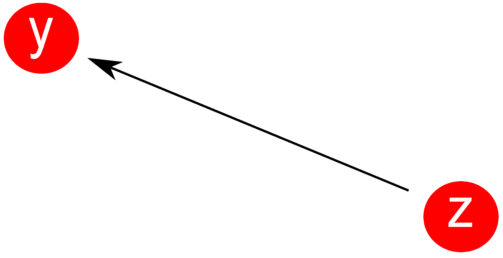
Definition 1

(Derivative). Let f be a function of $E\times {\mathbb{R}}_{+}$ in $\mathbb{R}$.1 The directional derivative of f from $z\in G$ to $y\in G$ is given by

$${\partial }_{z}f\left(y\right)=\left(f\left(y\right)-f\left(z\right)\right)a_{yz}.$$

(3)

The operator ${\partial }_z$ is a linear map of f, for any $z\in G$.

Figure 2 represents the derivative. The rest of the definitions depend on this, so it is important to well understand this last one.

Figure 2. The $\mathrm{directional}$ $\mathrm{derivative}$ of f from z to y. This actually represents the (finite) variation of f for the information going from node z to node y. It is positive if y gets more information than z, and negative otherwise. This concept makes sense only if y and z are neighbors; hence, the presence of $a_{yz}\in \{0,1\}$ in the definition.

Definition 2

(Gradient). Let $f:E\times {\mathbb{R}}_{+}\to \mathbb{R}$. The gradient of f at $y\in G$ is the vector given by 2

$${\nabla }^{y}f={\left({\partial }_{z}f\left(y\right)\right)}_{z\in \mathcal{N}\left(y\right)}=\left(\begin{array}{c}{\partial }_{1}f\left(y\right)\\ {\partial }_{2}f\left(y\right)\\ ⋮\\ {\partial }_{{\mathrm{d}}_{A}y}f\left(y\right)\end{array}\right).$$

(4)

The gradient at a node is the collection of directional derivatives toward this node.

Definition 3

(Laplacians). Let $f:E\times {\mathbb{R}}_{+}\to \mathbb{R}$. The normalized Laplacian of f from $x\in G$ to $y\in G$ is given by

$${\Delta }_{x}f\left(y\right)=\frac{1}{{\mathrm{d}}_{A}y}\sum _{z\in \mathcal{N}\left(x\right)}{\partial }_z{\partial }_{z}f\left(y\right),$$

(5)

while the non-normalized Laplacian of f from $x\in G$ to $y\in G$ is given by

$$L_{x}f\left(y\right)=\sum _{z\in \mathcal{N}\left(x\right)}{\partial }_z{\partial }_{z}f\left(y\right).$$

(6)

The global normalized Laplacian of f at x is given by

$$\Delta f\left(x\right)=\frac{1}{{\mathrm{d}}_{A}x}\sum _{z\in G}{\partial }_z{\partial }_{z}f\left(x\right),$$

(7)

while the global non-normalized Laplacian of f at x is given by

$$Lf\left(x\right)=\sum _{z\in G}{\partial }_z{\partial }_{z}f\left(x\right).$$

(8)

$Lf$ (or $\Delta f$) is said to be the Laplacian of f.

The Laplacian $\Delta$ of f is the average of the second directional derivative of f at node x, while the Laplacian L of f is the average of the second directional derivative of f at node x. We then could define the following operator:

Definition 4

(Divergence). Let $x\in G$ and $f_z:E\times {\mathbb{R}}_{+}\to \mathbb{R}$, $z\in \mathcal{N}\left(x\right)$ be ${\mathrm{d}}_{A}x$ functions. Define the vectorial function $f={\left(f_z\right)}_{z\in \mathcal{N}\left(x\right)}$. The divergence of f at $x\in G$ is given by

$${\nabla }^x·f=\sum _{z\in \mathcal{N}\left(x\right)}{f}_z\left(z\right),$$

(9)

or

$${\nabla }^x·f=\frac{1}{{\mathrm{d}}_{A}x}\sum _{z\in \mathcal{N}\left(x\right)}{f}_z\left(z\right),$$

(10)

depending on whether we choose L or Δ.

This is the sum (or average) value of f for a given node, the average being taken at each of the considered node’s neighbors.

Proposition 1

(Div of grad is Laplacian). For any $x\in G$, we have

$${\nabla }^x·{\nabla }^{x}f=L_{x}f\mathrm{or}{\Delta }_{x}f,$$

(11)

depending on whether we choose $L_x$ or ${\Delta }_x$ for the definition of the divergence.

Proof. 

Note that, for all $y,z\in G$, we have

$$\begin{array}{cc}\hfill {\partial }_z{\partial }_{z}f\left(y\right)& ={\partial }_z\left(\left(f\left(y\right)-f\left(z\right)\right)a_{yz}\right)\hfill \\ \hfill & =\left({\partial }_{z}f\left(y\right)-{\partial }_{z}f\left(z\right)\right)a_{yz}\hfill \\ \hfill & =\left(\left(f\left(y\right)-f\left(z\right)\right)a_{yz}-0\right)a_{yz}\hfill \\ \hfill & =\left(f\left(y\right)-f\left(z\right)\right)a_{yz}^2.\hfill \end{array}$$

Since $a_{yz}^2=a_{yz}\in \{0,1\}$, we therefore have that ${\partial }_z{\partial }_{z}f\left(y\right)={\partial }_{z}f\left(y\right)$. It turns out that ${\nabla }^x·{\nabla }^{x}f={\Delta }_{x}f$, or $\nabla ·\nabla =\Delta$. □

Thus, we note that ${\partial }_z{\partial }_z={\partial }_z$, and it turns out that $\Delta f\left(x\right)={\Delta }_{x}f\left(x\right)$, for any $x\in G$. A straightforward but essential property for the Laplacian is depicted as follows.

Proposition 2.

Let $f:E\times {\mathbb{R}}_{+}\to \mathbb{R}$. The Laplacians of f at $x\in G$ satisfy the following property:

$$Lf\left(x\right)={\mathrm{d}}_{A}xf\left(x\right)-\sum _{z\in \mathcal{N}\left(x\right)}f\left(z\right),$$

(12)

$$\Delta f\left(x\right)=f\left(x\right)-\frac{1}{{\mathrm{d}}_{A}x}\sum _{z\in \mathcal{N}\left(x\right)}f\left(z\right).$$

(13)

Thus, the Laplacian of f at x is the value of f at x, minus the average value of f taken by all its neighbors.

Proof. 

From the definition, and since $a_{xz}=1$ if and only if $z\in \mathcal{N}\left(x\right)$, we have

$$\Delta f\left(x\right)=\frac{1}{{\mathrm{d}}_{A}x}\sum _{z\in \mathcal{N}\left(x\right)}{\partial }_z{\partial }_{z}f\left(x\right)=\frac{1}{{\mathrm{d}}_{A}x}\left(\sum _{z\in \mathcal{N}\left(x\right)}f\left(x\right)-\sum _{z\in \mathcal{N}\left(x\right)}f\left(z\right)\right),$$

which implies the results. □

This actually allows to introduce the Laplacian matrix.

Definition 5

(Laplacian matrix). The non-normalized Laplacian matrix is given by

$$L=\mathcal{D}-A,$$

(14)

where A is the adjacency matrix, and $\mathcal{D}=\mathrm{diag}({\mathrm{d}}_{A}x,{\mathrm{d}}_{A}y,\dots )$ is the diagonal matrix of degrees.

The Laplacian matrix is given by

$$\Delta ={\mathcal{D}}^{-1}L=1-{\mathcal{D}}^{-1}A,$$

(15)

where 1 is the identity matrix.

Contrary to any other field in mathematics, there are no criteria of derivability. The function just needs to be defined at the two considered points.

2.3. Integration

After having defined the derivatives, we have to define the integration.

Definition 6.

Let $f,h:E\to \mathbb{R}$. We introduce the map scalar product of f by h on any sub-graph $g\subseteq G$ of G, as follows:

$${⟨f,h⟩}_g=\sum _{x\in g}f\left(x\right)h\left(x\right).$$

(16)

The following proposition is straightforward, but fundamental.

Proposition 3

(Scalar product). The map ${⟨·,·⟩}_g:f,h\mapsto {⟨f,h⟩}_g$ is a bilinear form from $E^2$ to $\mathbb{R}$, for any $g\subseteq G$. This justifies its name scalar product. Thus, the family $(G,⟨·,·⟩)$ is said to be a Euclidean graph.

In the following, the graph G is always considered a Euclidean graph.

Definition 7

(Integration). Let $f:E\to \mathbb{R}$. We introduce the integration of f on any sub-graph $g\subseteq G$ of G, as follows:

$${\int }_{g}f{\mathrm{d}}_A=⟨f,{\mathrm{d}}_A⟩=\sum _{x\in g}f\left(x\right)d_{A}x.$$

(17)

${\mathrm{d}}_A$ is a measure on G by $⟨·,·⟩$.

Here again, the function, to be integrable in g, just needs to be defined on g. The previous and following properties are still satisfied for a function $f:E\times {\mathbb{R}}_{+}\to \mathbb{R}$.

The above definition actually is consistent with integration by parts.

Proposition 4

(Integration by parts). Let $f,h:E\to \mathbb{R}$. We have

$${\int }_{\mathcal{N}\left(x\right)}h{\Delta }_{x}f{\mathrm{d}}_A={\int }_{\mathcal{N}\left(x\right)}{\Delta }_{x}hf{\mathrm{d}}_A,$$

(18)

$${\int }_{G}h\Delta f{\mathrm{d}}_A={\int }_G\Delta hf{\mathrm{d}}_A.$$

(19)

Proof. 

We calculate

$$\begin{array}{cc}\hfill {\int }_{\mathcal{N}\left(x\right)}h{\Delta }_{x}f{\mathrm{d}}_A& =\sum _{y\in \mathcal{N}\left(x\right)}h\left(y\right){\Delta }_{x}f\left(y\right){\mathrm{d}}_{A}y=\sum _{y\in \mathcal{N}\left(x\right)}\sum _{z\in \mathcal{N}\left(x\right)}h\left(y\right)(f\left(y\right)-f\left(z\right))\hfill \\ \hfill & =\frac{1}{2}\sum _{y\in \mathcal{N}\left(x\right)}\sum _{z\in \mathcal{N}\left(x\right)}h\left(y\right)(f\left(y\right)-f\left(z\right))+\frac{1}{2}\sum _{y\in \mathcal{N}\left(x\right)}\sum _{z\in \mathcal{N}\left(x\right)}h\left(z\right)(f\left(z\right)-f\left(y\right))\hfill \\ \hfill & =\frac{1}{2}\sum _{y\in \mathcal{N}\left(x\right)}\sum _{z\in \mathcal{N}\left(x\right)}(h\left(y\right)-h\left(z\right))(f\left(y\right)-f\left(z\right))\hfill \\ \hfill & =\sum _{y\in \mathcal{N}\left(x\right)}\sum _{z\in \mathcal{N}\left(x\right)}(h\left(y\right)-h\left(z\right))f\left(y\right)=\sum _{y\in \mathcal{N}\left(x\right)}{\Delta }_{x}h\left(y\right)f\left(y\right){\mathrm{d}}_{A}y\hfill \\ \hfill & ={\int }_{\mathcal{N}\left(x\right)}{\Delta }_{x}hf{\mathrm{d}}_A.\hfill \end{array}$$

Equation (18) is proven. In addition, we have

$$\begin{array}{cc}\hfill {\int }_{G}h\Delta f{\mathrm{d}}_A& =\sum _{x\in G}h\left(x\right)\Delta f\left(x\right){\mathrm{d}}_{A}x\hfill \\ \hfill & =\sum _{x\in G}\sum _{y\in G}h\left(x\right)(f\left(x\right)-f\left(y\right))a_{xy}\hfill \\ \hfill & =\frac{1}{2}\sum _{x\in G}\sum _{y\in G}(h\left(x\right)-h\left(y\right))(f\left(x\right)-f\left(y\right))a_{xy},\hfill \end{array}$$

which aims at proving Equation (19) as was previously done. □

We now have all the tools to develop the diffusion theory on a network, which is the object of the next session.

3. The Diffusion Equation

3.1. Derivation of the Equation

In order to derive the diffusion equation, we need the following essential proposition. In the sequence, we call $f:E\times {\mathbb{R}}_{+}\to \mathbb{R}$ the number of hashes produced per miner, as a function of nodes and time.

Proposition 5.

The density of the current of hashes from at $x\in G$ at time t is given by the following law of diffusion:

$$j(t,x)=-D{\nabla }^{x}f(t,·),$$

(20)

where $D>0$ is the diffusion coefficient of information.

We indeed assume that D is constant and is a network characteristic. Despite the fact that this law is very intuitive and is a typical Fick law (the information goes toward where there is not any information yet and hence the negative sign), further developments need to be made to rigorously justify this equation in the context of the network. Let us write $j(t,x)={\left(j_z(t,x)\right)}_{z\in \mathcal{N}\left(x\right)}$ the vector j at x and t. Thus, $j_z(t,x)$ represents the flow of information from z to x.

Here is the first important result of the paper.

Theorem 1.

Let $f:E\times {\mathbb{R}}_{+}\to \mathbb{R}$ represent the information function. If D is the diffusion coefficient and $\mathsf{\Gamma }:E\times {\mathbb{R}}_{+}\to \mathbb{R}$ the creation function of the information, the following diffusion equation holds for any $x\in V$ and $t\in {\mathbb{R}}_{+}$:

$$\frac{\partial f}{\partial t}(t,x)=-DLf(t,x)+\mathsf{\Gamma }(t,x)$$

(21)

Separately, the following diffusion equation also is valid

$$\frac{\partial f}{\partial t}(t,x)=-D\Delta f(t,x)+\mathsf{\Gamma }(t,x)$$

(22)

As long as one remembers that it is local, these equations can simply be written as

$$\frac{\partial f}{\partial t}=-DLf+\mathsf{\Gamma },\frac{\partial f}{\partial t}=-D\Delta f+\mathsf{\Gamma }.$$

The minus sign is actually a necessity for the system to be described as diffusive, and not an explosive one, contrary to standard math and physics systems.

Proof. 

On the one hand, let $\delta N$ be the quantity of hashes produced during the infinitesimal variation of time $\mathrm{d}t$, at node $x\in G$. The hash rate is the flux of rates given by $\varphi =\delta N/\mathrm{d}t$, and the number of such hashes produced per neighbors, for node $x\in G$, from time t and $t+\mathrm{d}t$, is $f(t+\mathrm{d}t,x)-f(t,x)=\delta N/{\mathrm{d}}_{A}x$. It turns out that

$$\delta N=\frac{\partial f}{\partial t}(t,x)\mathrm{d}t{\mathrm{d}}_{A}x.$$

On the other hand, node x (i) receives the diffused information from its neighbor, implying $\delta N_{\mathrm{enter}}$ hashes, and (ii) can create (or destruct) information, implying $\delta N_{\mathrm{create}}$ hashes. We therefore must have the following conservation of information:

$$\delta N=\delta N_{\mathrm{entering}}+\delta N_{\mathrm{create}}.$$

(23)

On point (i), the quantity of information entering into node x is provided from all its neighbors, and thus ${\displaystyle \delta N_{\mathrm{entering}}=\sum _{z\in \mathcal{N}\left(x\right)}{j}_z(t,x)\mathrm{d}t}$. On point (ii), we introduce the creation rate per node $\mathsf{\Gamma }(t,x)$ at node x and time t, which is the rate per node per second hashes are calculated. We therefore have $\delta N_{\mathrm{create}}=\mathsf{\Gamma }(t,x)\mathrm{d}t{\mathrm{d}}_{A}x$.

Bearing all the above in mind, Equation (23) becomes

$$\frac{\partial f}{\partial t}(t,x)\mathrm{d}t{\mathrm{d}}_{A}x=\sum _{z\in \mathcal{N}\left(x\right)}{j}_z(t,x)\mathrm{d}t+\mathsf{\Gamma }(t,x)\mathrm{d}t{\mathrm{d}}_{A}x,$$

Equivalently,

$$\frac{\partial f}{\partial t}(t,x)=\frac{1}{{\mathrm{d}}_{A}x}\sum _{z\in \mathcal{N}\left(x\right)}{j}_z(t,x)+\mathsf{\Gamma }(t,x),$$

or

$$\frac{\partial f}{\partial t}(t,x)={\nabla }^x·j(t,x)+\mathsf{\Gamma }(t,x).$$

According to Proposition 5, we have ${\nabla }^x·j(t,x)=-D\Delta f(t,x)$ or $L\Delta f(t,x)$, which does conclude the proof. □

3.2. Laplacian Matrix: Eigenvalues/Eigenvectors

3.2.1. Quick reminder: Eigenvalues/Eigenvectors

Let $G=(E,V)$ be a graph, with $n\in \mathbb{N}$ nodes and the adjacency matrix A, and $F:E^n\to E^n$. We say that $\lambda \in \mathbb{C}$ is an eigenvalue of F if the function $F-\lambda Id$ ($Id$ is the identity map) is not injective, which means that there exists a vector $V\in {\mathbb{R}}^n$, named eigenvector, such that $F\left(V\right)=\lambda V$, or component-wise $F\left(V\right(x\left)\right)=\lambda V\left(x\right)$ for $x\in G$. The function F has n eigenvalues, which we write ${\lambda }_1$, ${\lambda }_2$, …, ${\lambda }_n$, the index being chosen such that $|{\lambda }_1|\ge |{\lambda }_2|\ge \dots \ge |{\lambda }_n|\ge 0$. To each eigenvalue ${\lambda }_i$, we associate its eigenvector $V_i$, for all $\{1,2,\dots ,n\}$.

Separately, the function F can be seen as a matrix M, and the above equation is thus written as $MV=\lambda V$, or component-wise $MV\left(x\right)=\lambda V\left(x\right)$. We adapt to the matrix viewpoint in the following. If M is symmetric, then it is diagonalizable and ${\left(V_i\right)}_{i\in \{1,2,\dots ,n\}}$ is an orthonormal basis of ${\mathbb{R}}^n$, that is

$${⟨V_i,V_j⟩}_G=\sum _{x\in G}{V}_i\left(x\right)V_j\left(x\right)={\delta }_{ij},$$

(24)

where ${\delta }_{ij}$ is the Kronecker symbol.

3.2.2. Laplacian: Eigenvalues/Eigenvectors

The above applies to the Laplacian matrix (see Definition 5). For instance, the non-normalized Laplacian matrix for Figure 1 writes as

$$L=\left(\begin{array}{ccccccccc}1& -1& -1& 0& 0& 0& 0& 0& 0\\ -1& 1& -1& 0& 0& 0& 0& 0& 0\\ -1& -1& 1& -1& -1& -1& 0& 0& 0\\ 0& 0& -1& 1& 0& 0& 0& 0& 0\\ 0& 0& -1& 0& 1& -1& 0& 0& 0\\ 0& 0& -1& 0& -1& 1& -1& 0& 0\\ 0& 0& 0& 0& 0& -1& 1& -1& -1\\ 0& 0& 0& 0& 0& 0& -1& 1& 0\\ 0& 0& 0& 0& 0& 0& -1& 0& 1\end{array}\right).$$

(25)

The matrix L is symmetric and positive (semi-)definite. We write ${\left({\mu }_i\right)}_{i\in \{1,2,\dots ,n\}}$ the eigenvalues of the matrix L such that ${\mu }_1\ge {\mu }_2\ge \dots \ge {\mu }_n\ge 0$ with the associated eigenvalues ${\left(v_i\right)}_{i\in \{1,2,\dots ,n\}}$, forming an orthonormal basis of ${\mathbb{R}}^n$. The normalized Laplacian matrix writes

$$\Delta =\left(\begin{array}{ccccccccc}1& -1/2& -1/2& 0& 0& 0& 0& 0& 0\\ -1/2& 1& -1/2& 0& 0& 0& 0& 0& 0\\ -1/5& -1/5& 1& -1/5& -1/5& -1/5& 0& 0& 0\\ 0& 0& -1& 1& 0& 0& 0& 0& 0\\ 0& 0& -1/2& 0& 1& -1/2& 0& 0& 0\\ 0& 0& -1/3& 0& -1/3& 1& -1/3& 0& 0\\ 0& 0& 0& 0& 0& -1/3& 1& -1/3& -1/3\\ 0& 0& 0& 0& 0& 0& -1& 1& 0\\ 0& 0& 0& 0& 0& 0& -1& 0& 1\end{array}\right).$$

(26)

The matrix $\Delta$ is only positive semi-definite.

In the sequence, we focus our attention on the matrix $\tilde{\Delta }={\mathcal{D}}^{1/2}\Delta {\mathcal{D}}^{-1/2}$. This matrix is positive semi-definite, but also, since $\tilde{\Delta }={\mathcal{D}}^{1/2}{\mathcal{D}}^{-1}L{\mathcal{D}}^{-1/2}={\mathcal{D}}^{-1/2}L{\mathcal{D}}^{-1/2}$, it is symmetric. As an example, we have

$$\tilde{\Delta }=\left(\begin{array}{ccccccccc}1& -1/\sqrt{2}& -1/\sqrt{10}& 0& 0& 0& 0& 0& 0\\ -1/\sqrt{2}& 1& -1/\sqrt{10}& 0& 0& 0& 0& 0& 0\\ -1/\sqrt{10}& -1/\sqrt{10}& 1& -1/\sqrt{5}& -1/\sqrt{10}& -1/\sqrt{15}& 0& 0& 0\\ 0& 0& -1/\sqrt{5}& 1& 0& 0& 0& 0& 0\\ 0& 0& -1/\sqrt{10}& 0& 1& -1/\sqrt{6}& 0& 0& 0\\ 0& 0& -1/\sqrt{15}& 0& -1/\sqrt{6}& 1& -1/3& 0& 0\\ 0& 0& 0& 0& 0& -1/3& 1& -1/\sqrt{3}& -/\sqrt{3}\\ 0& 0& 0& 0& 0& 0& -1/\sqrt{3}& 1& 0\\ 0& 0& 0& 0& 0& 0& -1/\sqrt{3}& 0& 1\end{array}\right).$$

(27)

We write ${\left({\lambda }_i\right)}_{i\in \{1,2,\dots ,n\}}$ the eigenvalues of the matrix $\tilde{\Delta }$ such that ${\lambda }_1\ge {\lambda }_2\ge \dots \ge {\lambda }_n\ge 0$ with the associated eigenvalues ${\left(V_i\right)}_{i\in \{1,2,\dots ,n\}}$, forming an orthonormal basis of ${\mathbb{R}}^n$. The graph G is fully connected; therefore ${\lambda }_n=0$.

It is interesting to further develop the eigenvector $V_n$ associated with the eigenvalue ${\lambda }_n=0$. Set $v_n$ as the eigenvector of L associated with the eigenvalue ${\lambda }_n={\mu }_n=0$ (same common eigenvalue between L and $\tilde{\Delta }$). In addition, we have $L{v}_n=0$; hence, $\mathcal{D}{v}_n=A{v}_n$, which implies that $v_n=e/\sqrt{n}$ with the appropriate normalization.

Actually, we easily can establish that

$$\tilde{\Delta }{\mathcal{D}}^{1/2}{v}_n={\lambda }_n{\mathcal{D}}^{-1}{\mathcal{D}}^{1/2}{v}_n=0={\lambda }_n{\mathcal{D}}^{1/2}{v}_n.$$

It turns out that $V_n={\mathcal{D}}^{1/2}{v}_n$, and with the appropriate normalization, we finally have

$$V_n\left(x\right)=\sqrt{\frac{{\mathrm{d}}_{A}x}{\mathrm{Vol}\left(G\right)}}.$$

(28)

Two additional points to bear in mind are that $\tilde{\Delta }$ is equivalent to $\Delta$ by construction; therefore, both matrices have the same eigenvalues. Finally, since $\tilde{\Delta }={\mathcal{D}}^{-1/2}L{\mathcal{D}}^{-1/2}$, then, according to Sylvester’s inertia theorem, $\tilde{\Delta }$ and L, and thus $\Delta$, have the same number of negative, zero, and positive eigenvalues. Further developments can be done here.

3.3. Resolution of the Equation

We need the following lemma

Lemma 1.

The operator L is self-adjoint, in the sense that

$${⟨h,L_{x}f⟩}_{\mathcal{N}\left(x\right)}={⟨L_{x}h,f⟩}_{\mathcal{N}\left(x\right)},$$

(29)

$${⟨h,Lf⟩}_G={⟨Lh,f⟩}_G.$$

(30)

In addition, the operator $\tilde{\Delta }$ also is self-adjoint

$${⟨h,{\tilde{\Delta }}_{x}f⟩}_{\mathcal{N}\left(x\right)}={⟨{\tilde{\Delta }}_{x}h,f⟩}_{\mathcal{N}\left(x\right)},$$

(31)

$${⟨h,\tilde{\Delta }f⟩}_G={⟨\tilde{\Delta }h,f⟩}_G.$$

(32)

Proof. 

The first two equations have proofs very similar to the one for Proposition 4. We thus focus on ${\tilde{\Delta }}_x$ and $\tilde{\Delta }$.

First we note, for any $x\in G$, that

$$\tilde{\Delta }f\left(x\right)=f\left(x\right)-\frac{1}{\sqrt{{\mathrm{d}}_{A}x}}\sum _{z\in \mathcal{N}\left(x\right)}\frac{f\left(z\right)}{\sqrt{{\mathrm{d}}_{A}z}}=\frac{1}{\sqrt{{\mathrm{d}}_{A}x}}\sum _{z\in \mathcal{N}\left(x\right)}\left(\frac{f\left(x\right)}{\sqrt{{\mathrm{d}}_{A}x}}-\frac{f\left(z\right)}{\sqrt{{\mathrm{d}}_{A}z}}\right).$$

It turns out that

$${\tilde{\Delta }}_{x}f\left(y\right)=\frac{1}{\sqrt{{\mathrm{d}}_{A}y}}\sum _{z\in \mathcal{N}\left(x\right)}\left(\frac{f\left(y\right)}{\sqrt{{\mathrm{d}}_{A}y}}-\frac{f\left(z\right)}{\sqrt{{\mathrm{d}}_{A}z}}\right)a_{yz},\forall y\in G.$$

Bearing this in mind, we calculate

$$\begin{array}{cc}\hfill {⟨h,{\tilde{\Delta }}_{x}f⟩}_{\mathcal{N}\left(x\right)}& =\sum _{y\in \mathcal{N}\left(x\right)}h\left(y\right){\tilde{\Delta }}_{x}f\left(y\right)=\sum _{y\in \mathcal{N}\left(x\right)}h\left(y\right)\frac{1}{\sqrt{{\mathrm{d}}_{A}y}}\sum _{z\in \mathcal{N}\left(x\right)}\left(\frac{f\left(y\right)}{\sqrt{{\mathrm{d}}_{A}y}}-\frac{f\left(z\right)}{\sqrt{{\mathrm{d}}_{A}z}}\right)a_{yz}\hfill \\ \hfill & =\sum _{y\in \mathcal{N}\left(x\right)}\sum _{z\in \mathcal{N}\left(x\right)}\frac{h\left(y\right)}{\sqrt{{\mathrm{d}}_{A}y}}\left(\frac{f\left(y\right)}{\sqrt{{\mathrm{d}}_{A}y}}-\frac{f\left(z\right)}{\sqrt{{\mathrm{d}}_{A}z}}\right)a_{yz}\hfill \\ \hfill & =\frac{1}{2}\sum _{y\in \mathcal{N}\left(x\right)}\sum _{z\in \mathcal{N}\left(x\right)}\frac{h\left(y\right)}{\sqrt{{\mathrm{d}}_{A}y}}\left(\frac{f\left(y\right)}{\sqrt{{\mathrm{d}}_{A}y}}-\frac{f\left(z\right)}{\sqrt{{\mathrm{d}}_{A}z}}\right)a_{yz}\hfill \\ \hfill & +\frac{1}{2}\sum _{y\in \mathcal{N}\left(x\right)}\sum _{z\in \mathcal{N}\left(x\right)}\frac{h\left(z\right)}{\sqrt{{\mathrm{d}}_{A}z}}\left(\frac{f\left(z\right)}{\sqrt{{\mathrm{d}}_{A}z}}-\frac{f\left(y\right)}{\sqrt{{\mathrm{d}}_{A}y}}\right)a_{zy}\hfill \\ \hfill & =\frac{1}{2}\sum _{y\in \mathcal{N}\left(x\right)}\sum _{z\in \mathcal{N}\left(x\right)}\left(\left(\frac{h\left(y\right)}{\sqrt{{\mathrm{d}}_{A}y}}-\frac{h\left(z\right)}{\sqrt{{\mathrm{d}}_{A}z}}\right)a_{yz}\times \left(\frac{f\left(y\right)}{\sqrt{{\mathrm{d}}_{A}y}}-\frac{f\left(z\right)}{\sqrt{{\mathrm{d}}_{A}z}}\right)a_{yz}\right)\hfill \\ \hfill & =\sum _{y\in \mathcal{N}\left(x\right)}\sum _{z\in \mathcal{N}\left(x\right)}\left(\frac{h\left(y\right)}{\sqrt{{\mathrm{d}}_{A}y}}-\frac{h\left(z\right)}{\sqrt{{\mathrm{d}}_{A}z}}\right)a_{yz}\frac{f\left(y\right)}{\sqrt{{\mathrm{d}}_{A}y}}\hfill \\ \hfill & =\sum _{y\in \mathcal{N}\left(x\right)}{\tilde{\Delta }}_{x}h\left(y\right)f\left(y\right)={⟨{\tilde{\Delta }}_{x}h,f⟩}_{\mathcal{N}\left(x\right)}.\hfill \end{array}$$

Equation (31) is proven. For Equation (32), we have

$$\begin{array}{cc}\hfill {⟨h,\tilde{\Delta }f⟩}_G& =\sum _{x\in G}h\left(x\right)\tilde{\Delta }f\left(x\right)=\sum _{x\in G}h\left(x\right)\frac{1}{\sqrt{{\mathrm{d}}_{A}x}}\sum _{y\in G}\left(\frac{f\left(x\right)}{\sqrt{{\mathrm{d}}_{A}x}}-\frac{f\left(y\right)}{\sqrt{{\mathrm{d}}_{A}y}}\right)a_{xy}\hfill \\ \hfill & =\frac{1}{2}\sum _{x\in G}\sum _{y\in G}\left(\left(\frac{h\left(x\right)}{\sqrt{{\mathrm{d}}_{A}x}}-\frac{h\left(y\right)}{\sqrt{{\mathrm{d}}_{A}y}}\right)a_{xy}\times \left(\frac{f\left(x\right)}{\sqrt{{\mathrm{d}}_{A}x}}-\frac{f\left(y\right)}{\sqrt{{\mathrm{d}}_{A}y}}\right)a_{xy}\right),\hfill \end{array}$$

which aims at proving the result, as previously done. □

Here is the second important result of the paper. We have the following analytical expression for the hash rate per node.

Theorem 2.

The solution for the diffusion Equation (21) is given by

$$f(t,x)=\sum _{i=1}^n\left(C_i^L{\mathrm{e}}^{-D{\mu }_{i}t}+{\int }_0^t{\mathrm{e}}^{-D{\mu }_i(t-\tau )}{⟨\mathsf{\Gamma }(\tau ,·),v_i⟩}_G\mathrm{d}\tau \right)v_i\left(x\right)$$

(33)

with $(C_1^L,C_2^L,\dots ,C_n^L)\in {\mathbb{R}}^n$.

The solution for the diffusion Equation (22) is given by

$$f(t,x)=\frac{1}{\sqrt{{\mathrm{d}}_{A}x}}\sum _{i=1}^n\left(C_i^{\tilde{\Delta }}{\mathrm{e}}^{-D{\lambda }_{i}t}+{\int }_0^t{\mathrm{e}}^{-D{\lambda }_i(t-\tau )}{⟨{\mathcal{D}}^{1/2}\mathsf{\Gamma }(\tau ,·),V_i⟩}_G\mathrm{d}\tau \right)V_i\left(x\right)$$

(34)

with $(C_1^{\tilde{\Delta }},C_2^{\tilde{\Delta }},\dots ,C_n^{\tilde{\Delta }})\in {\mathbb{R}}^n$.

It is worth pointing out that these analytical solutions easily are implementable in a computer.

Proof. 

We first focus on the solution for Equation (21). We decompose $f(t,x)$ into the basis ${\left(v_i\right)}_{i\in \{1,2,\dots ,n\}}$ of ${\mathbb{R}}^n$ made of eigenvectors of the matrix L.

$$f(t,x)=\sum _{i=1}^n{\alpha }_i\left(t\right)v_i\left(x\right),$$

(35)

where, for all $i\in \{1,2,\dots ,n\}$, we have

$${\alpha }_i\left(t\right)={⟨f,v_i⟩}_G.$$

We have

$${⟨f,L{v}_i⟩}_G={\mu }_i{⟨f,v_i⟩}_G={\mu }_i{\alpha }_i\left(t\right).$$

Using Lemma 1, we have

$${\mu }_i{\alpha }_i\left(t\right)={⟨Lf,v_i⟩}_G={⟨Lf,v_i⟩}_G,$$

and using Equation (21), we have

$$-D{\mu }_i{\alpha }_i\left(t\right)={⟨\frac{\partial f}{\partial t}(t,·),v_i⟩}_G-{⟨\mathsf{\Gamma }(t,·),v_i⟩}_G.$$

Implementing Equation (35), we have

$$\begin{array}{cc}\hfill -D{\mu }_i{\alpha }_i\left(t\right)& =\frac{\mathrm{d}}{\mathrm{d}t}\sum _{j=1}^n{\alpha }_j\left(t\right){⟨v_j,v_i⟩}_G-{⟨\mathsf{\Gamma }(t,·),v_i⟩}_G.\hfill \\ \hfill ⟺D{\mu }_i{\alpha }_i\left(t\right)& =-\frac{\mathrm{d}}{\mathrm{d}t}\sum _{j=1}^n{\alpha }_j\left(t\right){\delta }_{ij}+{⟨\mathsf{\Gamma }(t,·),v_i⟩}_G\hfill \\ \hfill & =-\frac{\mathrm{d}{\alpha }_i\left(t\right)}{\mathrm{d}t}+{⟨\mathsf{\Gamma }(t,·),v_i⟩}_G.\hfill \\ \hfill ⟺\frac{\mathrm{d}{\alpha }_i\left(t\right)}{\mathrm{d}t}& =-D{\mu }_i{\alpha }_i\left(t\right)+{⟨\mathsf{\Gamma }(t,·),v_i⟩}_G.\hfill \end{array}$$

We can easily solve this differential equation, and we have

$${\alpha }_i\left(t\right)={\alpha }_i\left(0\right){\mathrm{e}}^{-D{\mu }_{i}t}+{\int }_0^t{\mathrm{e}}^{-D{\mu }_i(t-\tau )}{⟨\mathsf{\Gamma }(\tau ,·),v_i⟩}_G\mathrm{d}\tau .$$

We obtain the final result by placing the previous equation to Equation (35).

We now focus on the solution for Equation (22). We decompose $\left({\mathcal{D}}^{1/2}f\right)(t,x)$ into the basis ${\left(V_i\right)}_{i\in \{1,2,\dots ,n\}}$ of ${\mathbb{R}}^n$ made of eigenvectors of the matrix $\tilde{\Delta }$. The rest of the calculation remains exactly the same as below, with the additional trick $\tilde{\Delta }{\mathcal{D}}^{1/2}={\mathcal{D}}^{1/2}\Delta$. □

We note that $C_i^L=C_i^{\tilde{\Delta }}/\sqrt{{\mathrm{d}}_{A}x}$, for any $i\in 〚1,n〛$ and $x\in G$. It turns out that if $\mathsf{\Gamma }=0$, using L or $\Delta$ leads to the exact same result.

Corollary 1.

The solution for the diffusion Equation (21) is written as

$$f(t,x)={⟨f(0,·),{\mathcal{U}}^L(t,x,·)⟩}_G+{\int }_0^t{⟨\mathsf{\Gamma }(t-\tau ,·),{\mathcal{U}}^L(\tau ,x,·)⟩}_G\mathrm{d}\tau$$

(36)

$$f(t,x)={⟨f(0,·),{\mathcal{U}}^{\tilde{\Delta }}(t,x,·)⟩}_G+{\int }_0^t{⟨\mathsf{\Gamma }(t-\tau ,·),{\mathcal{U}}^{\tilde{\Delta }}(\tau ,x,·)⟩}_G\mathrm{d}\tau$$

(37)

where ${\mathcal{U}}^L:{\mathbb{R}}_{+}\times E^2\to \mathbb{R}$ is the diffusion propagator for the matrix L, and is such that

$${\mathcal{U}}^L(t,x,y)=\sum _{i=1}^n{\mathrm{e}}^{-D{\mu }_{i}t}{v}_i\left(x\right)v_i\left(y\right),\forall (t,x,y)\in {\mathbb{R}}_{+}\times E^2.$$

(38)

We also have

$${\mathcal{U}}^{\tilde{\Delta }}(t,x,y)=\sqrt{\frac{{\mathrm{d}}_{A}y}{{\mathrm{d}}_{A}x}}\sum _{i=1}^n{\mathrm{e}}^{-D{\lambda }_{i}t}{V}_i\left(x\right)V_i\left(y\right),\forall (t,x,y)\in {\mathbb{R}}_{+}\times E^2.$$

(39)

The advantage of this last expression is the explicit dependency of f with respect to the initial condition on all the nodes of G, i.e., with $f(0,y)$ for all $y\in G$.

Proof. 

We derive the expression for the matrix $\tilde{\Delta }$. From the general solution expression, we have

$$f(0,x)=\frac{1}{\sqrt{{\mathrm{d}}_{A}x}}\sum _{j=1}^n{C}_j{V}_j\left(x\right).$$

Therefore, we have

$$C_i={⟨V_i,\sqrt{{\mathrm{d}}_A}f(0,·)⟩}_G=\sum _{y\in G}{V}_i\left(y\right)\sqrt{{\mathrm{d}}_{A}y}f(0,y).$$

Implementing into the main solution expression, we have

$$\begin{array}{cc}\hfill f(t,x)=& \frac{1}{\sqrt{{\mathrm{d}}_{A}x}}\sum _{i=1}^n\left(\sum _{y\in G}{V}_i\left(y\right)\sqrt{{\mathrm{d}}_{A}y}f(0,y){\mathrm{e}}^{-D{\lambda }_{i}t}\right.\hfill \\ \hfill & \left.+{\int }_0^t\sum _{y\in G}\sqrt{{\mathrm{d}}_{A}y}{V}_i\left(y\right)\mathsf{\Gamma }(\tau ,y){\mathrm{e}}^{-D{\lambda }_i(t-\tau )}\mathrm{d}\tau \right)V_i\left(x\right).\hfill \end{array}$$

Some re-ordering leads to

$$\begin{array}{cc}\hfill f(t,x)=& \sum _{y\in G}\sqrt{\frac{{\mathrm{d}}_{A}y}{{\mathrm{d}}_{A}x}}\sum _{i=1}^n{V}_i\left(x\right)V_i\left(y\right)f(0,y){\mathrm{e}}^{-D{\lambda }_{i}t}\hfill \\ \hfill & +{\int }_0^t\sum _{y\in G}\sqrt{\frac{{\mathrm{d}}_{A}y}{{\mathrm{d}}_{A}x}}\sum _{i=1}^n{V}_i\left(x\right)V_i\left(y\right)\mathsf{\Gamma }(\tau ,y){\mathrm{e}}^{-D{\lambda }_i(t-\tau )}\mathrm{d}\tau .\hfill \end{array}$$

This explicitly is what we are looking for. A variable change will lead to the result. □

Remark 1.

We have

$${\mathcal{U}}^{\tilde{\Delta }}(0,x,y)=\sqrt{\frac{{\mathrm{d}}_{A}y}{{\mathrm{d}}_{A}x}}\sum _{i=1}^n{V}_i\left(x\right)V_i\left(y\right)=\sqrt{\frac{{\mathrm{d}}_{A}y}{{\mathrm{d}}_{A}x}}{\delta }_{xy}={\delta }_{xy},$$

where ${\delta }_{xy}=1$ if $x=y$ and 0 otherwise: the same for matrix L. We also have

$$\underset{t\to +\infty }{\lim }{\mathcal{U}}^{\tilde{\Delta }}(t,x,y)=\sqrt{\frac{{\mathrm{d}}_{A}y}{{\mathrm{d}}_{A}x}}{V}_n\left(x\right)V_n\left(y\right)=\sqrt{\frac{{\mathrm{d}}_{A}y}{{\mathrm{d}}_{A}x}}\sqrt{\frac{{\mathrm{d}}_{A}x}{\mathrm{Vol}\left(G\right)}}\sqrt{\frac{{\mathrm{d}}_{A}y}{\mathrm{Vol}\left(G\right)}}=\frac{{\mathrm{d}}_{A}y}{\mathrm{Vol}\left(G\right)},$$

in which case $\underset{t\to +\infty }{\lim }{\mathcal{U}}^{\tilde{\Delta }}(t,x,y)$ does not depend on x. We also found an interesting interpretation for the eigenvector $V_n$. Indeed, we have

$$\underset{t\to +\infty }{\lim }{\mathcal{U}}^{\tilde{\Delta }}(t,x,y)=V_n^2\left(y\right).$$

Therefore, $V_n^2\left(y\right)$ represents the propagation of information due to the diffusion, to node y.

The next two sections deal with further developments on the implications of the facts established above. This also holds for the operator L.

4. Standard Equilibrium and Blockchain Equilibrium

The equilibrium is an important aspect of the current paper. We identified two types of equilibrium, which we further develop here. The zero eigenvalue as well as its eigenvector will play an important role, as we are going to see.

4.1. Standard Equilibrium

4.1.1. Integrable Creation Destruction Function

The standard equilibrium corresponds to the steady state, i.e., when $t\to +\infty$. It is expected to have permanent exchanges between nodes at the same rate, which is exactly equivalent to the fact that each node keeps having the same quantity of information, i.e., the same quantity of hash generation.

More specifically, we have the following proposition.

Theorem 3

(Standard Equilibrium Framework). Let f be solution of the diffusion Equation (1). We assume that $t\mapsto \mathsf{\Gamma }(t,y)$ is integrable on ${\mathbb{R}}_{+}$ for any $y\in G$, and

$${\int }_0^t\mathsf{\Gamma }(\tau ,y){\mathrm{e}}^{-D{\lambda }_i(t-\tau )}\mathrm{d}\tau \underset{(t\to +\infty )}{\sim }{\gamma }_i\left(y\right),\mathrm{with}0\le {\gamma }_i\left(y\right)<+\infty ,\forall y\in G.$$

(40)

Then the standard equilibrium state corresponds to:

$$\underset{t\to +\infty }{\lim }f(t,x)=\frac{1}{\mathrm{Vol}\left(G\right)}\sum _{y\in G}{\mathrm{d}}_{A}y\left(f(0,y)+{\int }_0^{+\infty }\mathsf{\Gamma }(\tau ,y)\mathrm{d}\tau \right).$$

(41)

We have a similar result by considering the matrix L.

Proof. 

From the expression

$$\mathcal{U}(t,x,y)=\sqrt{\frac{{\mathrm{d}}_{A}y}{{\mathrm{d}}_{A}x}}\sum _{i=1}^n{\mathrm{e}}^{-D{\lambda }_{i}t}{V}_i\left(x\right)V_i\left(y\right),$$

we see that all the terms cancel since ${\lambda }_1\ge {\lambda }_2\ge \dots \ge {\lambda }_{n-1}>{\lambda }_n=0$, except the last one. Thus

$$\underset{t\to +\infty }{\lim }\mathcal{U}(t,x,y)=\sqrt{\frac{{\mathrm{d}}_{A}y}{{\mathrm{d}}_{A}x}}{V}_n\left(x\right)V_n\left(y\right)=\frac{{\mathrm{d}}_{A}y}{\mathrm{Vol}\left(G\right)}.$$

This does not depend on x. We then start from the following equation

$$\begin{array}{cc}\hfill f(t,x)=& \sum _{y\in G}\sqrt{\frac{{\mathrm{d}}_{A}y}{{\mathrm{d}}_{A}x}}\sum _{i=1}^n{V}_i\left(x\right)V_i\left(y\right)f(0,y){\mathrm{e}}^{-D{\lambda }_{i}t}\hfill \\ \hfill & +{\int }_0^t\sum _{y\in G}\sqrt{\frac{{\mathrm{d}}_{A}y}{{\mathrm{d}}_{A}x}}\sum _{i=1}^n{V}_i\left(x\right)V_i\left(y\right)\mathsf{\Gamma }(\tau ,y){\mathrm{e}}^{-D{\lambda }_i(t-\tau )}\mathrm{d}\tau .\hfill \end{array}$$

Hence,

$$\begin{array}{cc}\hfill \underset{t\to +\infty }{\lim }f(t,x)=& \frac{1}{\mathrm{Vol}\left(G\right)}\sum _{y\in G}{\mathrm{d}}_{A}yf(0,y)\hfill \\ \hfill & +\sum _{y\in G}\sqrt{\frac{{\mathrm{d}}_{A}y}{{\mathrm{d}}_{A}x}}\left[\sum _{i=1}^n{V}_i\left(x\right)V_i\left(y\right)\left(\underset{t\to +\infty }{\lim }{\int }_0^t\mathsf{\Gamma }(\tau ,y){\mathrm{e}}^{-D{\lambda }_i(t-\tau )}\mathrm{d}\tau \right)\right].\hfill \end{array}$$

The previous equation is the most general one. We come to the factor between parenthesis. The previous equation is then

$$\underset{t\to +\infty }{\lim }f(t,x)=\frac{1}{\mathrm{Vol}\left(G\right)}\sum _{y\in G}{\mathrm{d}}_{A}yf(0,y)+\sum _{y\in G}\sqrt{\frac{{\mathrm{d}}_{A}y}{{\mathrm{d}}_{A}x}}\left[\sum _{i=1}^n{V}_i\left(x\right)V_i\left(y\right){\gamma }_i\left(y\right)\right].$$

We now focus on the Equations (40). We will prove that ${\gamma }_i\left(y\right)=0$, for all $i\in \{1,\dots ,n-1\}$ and $y\in G$, which will prove Equation (41). A variable change gives

$${\int }_0^t\mathsf{\Gamma }(\tau ,y){\mathrm{e}}^{-D{\lambda }_i(t-\tau )}\mathrm{d}\tau ={\int }_0^t\mathsf{\Gamma }(t-\tau ,y){\mathrm{e}}^{-D{\lambda }_i\tau }\mathrm{d}\tau .$$

Bearing this in mind, for $i=n$, we have

$${\int }_0^t\mathsf{\Gamma }(\tau ,y)\mathrm{d}\tau \underset{(t\to +\infty )}{\sim }{\gamma }_n\left(y\right),$$

that is

$${\int }_0^{+\infty }\mathsf{\Gamma }(\tau ,y)\mathrm{d}\tau ={\gamma }_n\left(y\right)<+\infty .$$

Hence $\left|\mathsf{\Gamma }\right(\tau ,y\left)\right|\le C\left(y\right)<+\infty$ with C function from G to $\mathbb{R}$, and $\underset{\tau \to +\infty }{\lim }\mathsf{\Gamma }(\tau ,y)=0$, for any $y\in G$. It turns out that for any $i\in \{1,2,\dots ,n-1\}$, we have

$$\forall ϵ>0\exists \tilde{\tau }>0\forall \tau >\tilde{\tau }\left|\mathsf{\Gamma }(\tau ,y)\right|<ϵ\frac{D{\lambda }_i}{C\left(y\right)+1},\forall y\in G.$$

Hence, for any $i\in \{1,2,\dots ,n-1\}$ and $t>\tau$, we have

$$\left|{\int }_{\tilde{\tau }}^t\mathsf{\Gamma }(\tau ,y){\mathrm{e}}^{-D{\lambda }_i(t-\tau )}\mathrm{d}\tau \right|<{\int }_{\tilde{\tau }}^t\left|\mathsf{\Gamma }(\tau ,y)\right|{\mathrm{e}}^{-D{\lambda }_i(t-\tau )}\mathrm{d}\tau <ϵ\frac{1-{\mathrm{e}}^{-D{\lambda }_i(t-\tilde{\tau })}}{C\left(y\right)+1}.$$

Hence

$$\left|{\int }_0^t\mathsf{\Gamma }(\tau ,y){\mathrm{e}}^{-D{\lambda }_i(t-\tau )}\mathrm{d}\tau -{\int }_0^{\tilde{\tau }}\mathsf{\Gamma }(\tau ,y){\mathrm{e}}^{-D{\lambda }_i(t-\tau )}\mathrm{d}\tau \right|<ϵ\frac{1-{\mathrm{e}}^{-D{\lambda }_i(t-\tilde{\tau })}}{C\left(y\right)+1}.$$

By a variable change and using triangular inequality, we have

$$\left|{\int }_0^t\mathsf{\Gamma }(\tau ,y){\mathrm{e}}^{-D{\lambda }_i(t-\tau )}\mathrm{d}\tau \right|<\left|{\int }_{t-\tilde{\tau }}^t\mathsf{\Gamma }(t-\tau ,y){\mathrm{e}}^{-D{\lambda }_i\tau }\mathrm{d}\tau \right|+ϵ\frac{1-{\mathrm{e}}^{-D{\lambda }_i(t-\tilde{\tau })}}{C\left(y\right)+1}.$$

In other words, we have

$$\left|{\int }_0^t\mathsf{\Gamma }(\tau ,y){\mathrm{e}}^{-D{\lambda }_i(t-\tau )}\mathrm{d}\tau \right|<C\left(y\right)\frac{{\mathrm{e}}^{-D{\lambda }_{i}t}-{\mathrm{e}}^{-D{\lambda }_i(t-\tilde{\tau })}}{D{\lambda }_i}+ϵ\frac{1-{\mathrm{e}}^{-D{\lambda }_i(t-\tilde{\tau })}}{C\left(y\right)+1}.$$

Suppose now that $t\in {\mathbb{R}}_{+}^{*}$ is such that

$$t=\max \left(-\frac{1}{D{\lambda }_i}\ln \left(ϵ\frac{D{\lambda }_i}{C\left(y\right)+1}\right),\tau \right).$$

Then we have

$$\left|{\int }_0^t\mathsf{\Gamma }(\tau ,y){\mathrm{e}}^{-D{\lambda }_i(t-\tau )}\mathrm{d}\tau \right|<ϵ.$$

Therefore,

$$\underset{t\to +\infty }{\lim }{\int }_0^t\mathsf{\Gamma }(\tau ,y){\mathrm{e}}^{-D{\lambda }_i(t-\tau )}\mathrm{d}\tau ={\gamma }_i\left(y\right)=0,$$

which concludes the proof. □

For example, set $\mathsf{\Gamma }(t,x)=P\left(t\right){\mathrm{e}}^{\alpha t}$, where P is a polynomial and $\alpha \in \mathbb{R}$ with some restrictions that we need to discover.

Let $n\in \mathbb{N}$. A quick calculation allows to establish that

$$\int {\tau }^n{\mathrm{e}}^{a\tau }\mathrm{d}\tau =\left\{\begin{array}{cc}{\displaystyle \sum _{j=0}^n{(-1)}^{n-j}{\left(\frac{1}{a}\right)}^{n-j+1}\frac{n!}{j!}{\tau }^{n-j}{\mathrm{e}}^{a\tau }+{\mathrm{C}}^{\mathrm{te}}}\hfill & \mathrm{if}a\ne 0\hfill \\ & \\ {\displaystyle \frac{{\tau }^{n+1}}{n+1}+{\mathrm{C}}^{\mathrm{te}}}\hfill & \mathrm{otherwise}\hfill \end{array}\right.$$

If we set $\mathsf{\Gamma }(\tau ,x)={\tau }^n{\mathrm{e}}^{\alpha \tau }$, then we deduce that

$${\mathrm{e}}^{-D{\lambda }_{i}t}{\int }_0^t{\tau }^n{\mathrm{e}}^{(D{\lambda }_i+\alpha )\tau }\mathrm{d}\tau =\left\{\begin{array}{cc}{\displaystyle \sum _{j=0}^n{(-1)}^{n-j}{\left(\frac{1}{D{\lambda }_i+\alpha }\right)}^{n-j+1}\frac{n!}{j!}{t}^{n-j}{\mathrm{e}}^{\alpha t}}\hfill & \mathrm{if}\alpha \ne -D{\lambda }_i\hfill \\ & \\ {\displaystyle {\mathrm{e}}^{-D{\lambda }_{i}t}\frac{t^{n+1}}{n+1}}\hfill & \mathrm{otherwise}\hfill \end{array}\right.$$

We deduce that, for ${\gamma }_i\left(y\right)$ to be finite, we need to have $\alpha \in {\mathbb{R}}_{-}^{*}$, while $n\in \mathbb{N}$ without restriction, and the degree of P is in $\mathbb{N}$. However, if $\alpha =0$, then we necessarily need to have $n=0$. The less negligible function $\mathsf{\Gamma }$ is thus $\mathsf{\Gamma }(t,x)=P\left(0\right)$, which is the only form giving a nonzero ${\gamma }_i\left(y\right)=0$.

Remark 2.

Equation (40) is actually close to the one found by applying the mean value theorem, provided $\mathsf{\Gamma }(·,y)$ is continuous for any $y\in G$: there exists $a_i\in [0,t]$ such that

$${\int }_0^t\mathsf{\Gamma }(\tau ,y){\mathrm{e}}^{D{\lambda }_i\tau }\mathrm{d}\tau =\frac{\mathsf{\Gamma }(a_i,y)}{D{\lambda }_i}({\mathrm{e}}^{D{\lambda }_{i}t}-1),\forall y\in G.$$

(42)

Thus, ${\gamma }_i\left(y\right)=\mathsf{\Gamma }(a_i,y)/D{\lambda }_i$, with $a\in {\mathbb{R}}_{+}^{*}$.

Remark 3.

General function theory might be interesting if one decides to break the assumption that $\mathsf{\Gamma }(·,y)$ is continuous.

4.1.2. Continuous-by-Parts Creation Destruction Function

If we require the solution f to be continuous at all times, then, according to the diffusion equation, $\mathsf{\Gamma }$ must be at least continuous by parts. In this case, the function $\mathsf{\Gamma }(·,x)$ is continuous by parts, for any $x\in E$, i.e., there are some points on the time axis ${\mathbb{R}}_{+}$ where the function $\mathsf{\Gamma }(·,x)$ is not continuous (discontinuity of first kind). In this case, for any $x\in G$, the function $\mathsf{\Gamma }(·,x)$ still is integrable on ${\mathbb{R}}_{+}$.

4.2. Blockchain Equilibrium (Approximation)

In fact, we have to consider that time is discretized, i.e., subdivided into interval of time which are of length 10 min approximately. Ten minutes is the average time needed for a miner to mine a new block in the Bitoin blockchain Lipton and Treccani (2021), and this could be changed to 15 s for the Ethereum blockchain. We will go to deeper detail to this point in the future, but approximately every 10 min, the blockchain equilibrium equation is satisfied. The following are functions of interest:

• $r_b$—b-block reward;
• c—cost per hash, supposed to be constant;
• $P_t$—price of one Bitcoin, in USD, at time t;
• $f_i$—fee for transaction $i\in I$, where I is the set of all transactions that will be stacked into block b;
• $N_b$—number of hashes in the network, for block b.

From these five variables, we can easily compute the revenues $R_b$ for block b, as follows.

$$R_b=\left(r_b+\sum _{i\in I}{f}_i\right)P_T.$$

(43)

We can compose the costs, more precisely the expected costs $C_b$, for block b, as well:

$$C_b=c{N}_b.$$

(44)

We have the blockchain equilibrium equation:

$$R_b=C_b\iff \left(r_b+\sum _{i\in I}{f}_i\right)P_T=c{N}_b.$$

(45)

Thus, $N_b$ is connected to $f(t,x)$, which gives the cost for forming a block. We can, in fact, make the assumption that the circulation of transaction lists within miners is very fast: it takes approximately 1 millisecond for the nodes to receive the transaction list from an original list. It is relevant to assume that the diffusion happens very fast once one miner has a transaction list to be sent, and that the diffusion coefficient D is very high. This is the blockchain equilibrium approximation: $D{\lambda }_{n-1}t\gg 1$, for any time t.

In other words, $D{\lambda }_{n-1}t$ is so high that ${\mathrm{e}}^{-D{\lambda }_{i}t}\underset{(D{\lambda }_{n-1}t\to +\infty )}{\sim }0$, for any $i\in \{1,2,\dots ,n-1\}$. Only the term corresponding to ${\lambda }_n=0$ survives.

Proposition 6

(Blockchain Equilibirum Approximation). Let f be solution of the diffusion Equation (1). We focus on $t\in [0,T]$, where T is set to be 10 min. Then the blockchain equilibrium state corresponds to

$$f(T,x)\underset{(D{\lambda }_{n-1}t\to +\infty )}{\sim }\frac{1}{\mathrm{Vol}\left(G\right)}\sum _{y\in G}{\mathrm{d}}_{A}y\left(f(0,y)+{\int }_0^T\mathsf{\Gamma }(\tau ,y)\mathrm{d}\tau \right).$$

(46)

We have a similar result by considering the matrix L.

It turns out that $f(T,x)$, which does not depend on x, is the same for all the nodes.

Proof. 

We have

$${\mathrm{e}}^{-D{\lambda }_i\tau }\underset{(D{\lambda }_{n-1}t\to +\infty )}{\sim }\left\{\begin{array}{cc}0\hfill & \mathrm{if}i\in \{1,2,\dots ,n-1\}\hfill \\ 1\hfill & \mathrm{if}i=n\hfill \end{array}\right.$$

and

$${\int }_0^t\mathsf{\Gamma }(\tau ,y){\mathrm{e}}^{-D{\lambda }_i(t-\tau )}\mathrm{d}\tau \underset{(D{\lambda }_{n-1}t\to +\infty )}{\sim }\left\{\begin{array}{cc}0\hfill & \mathrm{if}i\in \{1,2,\dots ,n-1\}\hfill \\ {\displaystyle {\int }_0^{+\infty }\mathsf{\Gamma }(\tau ,y)\mathrm{d}\tau }\hfill & \mathrm{if}i=n\hfill \end{array}\right.$$

We deduce the equation from

$$\begin{array}{cc}\hfill f(t,x)=& \sum _{y\in G}\sqrt{\frac{{\mathrm{d}}_{A}y}{{\mathrm{d}}_{A}x}}\sum _{i=1}^n{V}_i\left(x\right)V_i\left(y\right)f(0,y){\mathrm{e}}^{-D{\lambda }_{i}t}\hfill \\ \hfill & +\sum _{y\in G}\sqrt{\frac{{\mathrm{d}}_{A}y}{{\mathrm{d}}_{A}x}}\left[\sum _{i=1}^n{V}_i\left(x\right)V_i\left(y\right)\left({\int }_0^t\mathsf{\Gamma }(\tau ,y){\mathrm{e}}^{-D{\lambda }_i(t-\tau )}\mathrm{d}\tau \right)\right],\hfill \end{array}$$

which concludes the proof. □

Thus, $f(T,x)$ is to be associated to $N_b$. Finally, in essence, the standard equilibrium and blockchain equilibrium give the same results. In the following, ‘$f(T,·)$’ refers to the function at the equilibrium state.

5. Undirected Graph: Case Studies

5.1. 2 Nodes

As a quick application, suppose $E=\{x,y\}$, only two nodes, and $V=\left\{\right(x,y\left)\right\}$, one connection. Suppose $\mathsf{\Gamma }=0$, $f(0,x)=f_0\in {\mathbb{R}}_{+}$, $f(0,y)=0$. We have $V_1{\left(x\right)}^2+V_1{\left(y\right)}^2=1$, ${\lambda }_2=0$, and

$$\begin{array}{cc}\hfill f(t,x)& =f_0\mathcal{U}(t,x,x)=f_0{V}_1{\left(x\right)}^2{\mathrm{e}}^{-D{\lambda }_{1}t}+f_0{V}_2{\left(x\right)}^2,\hfill \\ \hfill f(t,y)& =f_0\mathcal{U}(t,y,x)=f_0{V}_1\left(x\right)V_1\left(y\right){\mathrm{e}}^{-D{\lambda }_{1}t}+f_0{V}_2\left(x\right)V_2\left(y\right).\hfill \end{array}$$

We can calculate the eigenvalues and eigenvectors for the network. The non-normalized Laplacian matrix is given by

$$L=\left(\begin{array}{cc}1& -1\\ -1& 1\end{array}\right)$$

and the Laplacian matrix by $\Delta =\tilde{\Delta }=L$. The eigenvalues are $\lambda =2$ and ${\lambda }_2=0$, and the eigenvectors are $V_1={}^t(1/\sqrt{2}-1/\sqrt{2})$ and $V_2={}^t(1/\sqrt{2}1/\sqrt{2})$. We finally obtain

$$\left\{\begin{array}{cc}f(t,x)\hfill & {\displaystyle =\frac{f_0}{2}\left(1+{\mathrm{e}}^{-2Dt}\right)}\hfill \\ & \\ f(t,y)\hfill & {\displaystyle =\frac{f_0}{2}\left(1-{\mathrm{e}}^{-2Dt}\right)}\hfill \end{array}\right.$$

See Figure 3 for a plot of these two solutions.

Figure 3. Illustration of the diffusion information for 2 nodes. The initial conditions are $\mathsf{\Gamma }=0$, $f(0,x)=f_0\in {\mathbb{R}}_{+}$, and $f(0,y)=0$. We set $D=1/2$, and $f_0=2$. Blue is for $f(t,x)$, while red is for $f(t,y)$.

The equilibrium is therefore given by

$$f(T,x)=f(T,y)=f_0/2.$$

Finally, due to the diffusion effect, both nodes share the same information at the equilibrium.

5.2. 3 Nodes

We set that $E=\{1,2,3\}$ and $V=\left\{\right(1,2),(2,3\left)\right\}$. The non-normalized Laplacian of such a matrix is

$$L=\left(\begin{array}{ccc}1& -1& 0\\ -1& 2& -1\\ 0& -1& 1\end{array}\right)$$

and is

$$\tilde{\Delta }={\mathcal{D}}^{-1/2}L{\mathcal{D}}^{-1/2}=\left(\begin{array}{ccc}1& -1/\sqrt{2}& 0\\ -1/\sqrt{2}& 2& -1/\sqrt{2}\\ 0& -1/\sqrt{2}& 1\end{array}\right).$$

The eigenvalues of $\tilde{\Delta }$ are the roots of the polynomial $(1-X)\left[{(1-X)}^2-(1-X)/2-1/2\right]$, that is ${\lambda }_1=2$, ${\lambda }_2=1$, and ${\lambda }_3=0$. The eigenvectors are $V_1={}^t(1/2-1/\sqrt{2}1/2)$, $V_2={}^t(1/\sqrt{2}0-1/\sqrt{2})$, and $V_3={}^t(1/21/\sqrt{2}1/2)$.

We set $\mathsf{\Gamma }=0$. In order to be very explicit, the propagators are written as, for $x=1$,

$$\left\{\begin{array}{cc}\mathcal{U}(t,1,1)\hfill & {\displaystyle =\frac{1}{4}+\frac{1}{2}{\mathrm{e}}^{-Dt}+\frac{1}{4}{\mathrm{e}}^{-2Dt}}\hfill \\ & \\ \mathcal{U}(t,1,2)\hfill & {\displaystyle =\frac{1}{2}-\frac{1}{2}{\mathrm{e}}^{-2Dt}}\hfill \\ & \\ \mathcal{U}(t,1,3)\hfill & {\displaystyle =\frac{1}{4}-\frac{1}{2}{\mathrm{e}}^{-Dt}+\frac{1}{4}{\mathrm{e}}^{-2Dt}}\hfill \end{array}\right.$$

for $x=2$

$$\left\{\begin{array}{cc}\mathcal{U}(t,2,1)\hfill & {\displaystyle =\frac{1}{4}-\frac{1}{4}{\mathrm{e}}^{-2Dt}}\hfill \\ & \\ \mathcal{U}(t,2,2)\hfill & {\displaystyle =\frac{1}{2}+\frac{1}{2}{\mathrm{e}}^{-2Dt}}\hfill \\ & \\ \mathcal{U}(t,2,3)\hfill & {\displaystyle =\frac{1}{4}-\frac{1}{4}{\mathrm{e}}^{-2Dt}}\hfill \end{array}\right.$$

and for $x=3$

$$\left\{\begin{array}{cc}\mathcal{U}(t,1,1)\hfill & {\displaystyle =\frac{1}{4}-\frac{1}{2}{\mathrm{e}}^{-Dt}+\frac{1}{4}{\mathrm{e}}^{-2Dt}}\hfill \\ & \\ \mathcal{U}(t,1,2)\hfill & {\displaystyle =\frac{1}{2}-\frac{1}{2}{\mathrm{e}}^{-2Dt}}\hfill \\ & \\ \mathcal{U}(t,1,3)\hfill & {\displaystyle =\frac{1}{4}+\frac{1}{2}{\mathrm{e}}^{-Dt}+\frac{1}{4}{\mathrm{e}}^{-2Dt}}\hfill \end{array}\right.$$

Therefore, we have

$$\left\{\begin{array}{cc}f(t,1)\hfill & {\displaystyle =f(0,1)\left({\displaystyle \frac{1}{4}+\frac{1}{4}{\mathrm{e}}^{-Dt}+\frac{1}{4}{\mathrm{e}}^{-2Dt}}\right)}\hfill \\ & \\ & +f(0,2)\left({\displaystyle \frac{1}{2}-\frac{1}{2}{\mathrm{e}}^{-2Dt}}\right)\hfill \\ & \\ & +f(0,3)\left({\displaystyle \frac{1}{4}-\frac{1}{4}{\mathrm{e}}^{-Dt}+\frac{1}{4}{\mathrm{e}}^{-2Dt}}\right)\hfill \\ & \\ f(t,2)\hfill & {\displaystyle =f(0,1)\left({\displaystyle \frac{1}{4}-\frac{1}{4}{\mathrm{e}}^{-2Dt}}\right)}\hfill \\ & \\ & +f(0,2)\left({\displaystyle \frac{1}{2}+\frac{1}{2}{\mathrm{e}}^{-2Dt}}\right)\hfill \\ & \\ & +f(0,3)\left({\displaystyle \frac{1}{4}-\frac{1}{4}{\mathrm{e}}^{-2Dt}}\right)\hfill \\ & \\ f(t,3)\hfill & {\displaystyle =f(0,1)\left({\displaystyle \frac{1}{4}-\frac{1}{4}{\mathrm{e}}^{-Dt}+\frac{1}{4}{\mathrm{e}}^{-2Dt}}\right)}\hfill \\ & \\ & +f(0,2)\left({\displaystyle \frac{1}{2}-\frac{1}{2}{\mathrm{e}}^{-2Dt}}\right)\hfill \\ & \\ & +f(0,3)\left({\displaystyle \frac{1}{4}+\frac{1}{4}{\mathrm{e}}^{-Dt}+\frac{1}{4}{\mathrm{e}}^{-2Dt}}\right)\hfill \end{array}\right.$$

Figure 4 plots the evolution of the three functions.

Figure 4. Illustration of the diffusion information for 3 nodes. Node 2 is connected to nodes 1 and 3, but nodes 1 and 3 are not connected. The initial conditions are $\mathsf{\Gamma }=0$, $f(0,1)=1$, $f(0,2)=2$ and $f(0,3)=0$. We set $D=1$. Blue is for $f(t,1)$, red is for $f(t,2)$, and yellow is for $f(t,3)$.

The equilibrium state corresponds to the following expressions.

$$f(T,1)=f(T,2)=f(T,3)=\frac{1}{4}f(0,1)+\frac{1}{2}f(0,2)+\frac{1}{4}f(0,3).$$

We are now going to propose the solutions for specific P2P networks. It is worth stressing that implementation of the above in a prototype is in progress.

6. Generalization to Directed Graphs

This section focuses on the generalization of what has been seen so far, but applied to a directed graph. Concretely, information between different layers of the whole Bitcoin network is directed. A very simple example is that the users layer is sending information to the P2P network as transaction lists, and they do not expect any information back to them since they are not miners. The diffusion is thus directed. This breaks the symmetry of the adjacency matrix, which is not diagonalizable anymore. Thus, we could handle a more general framework to perform the diffusion. So far, we may handle with straight numerical solutions for the implementation, but we are going to see that we can derive an analytical solution base on the singular value decomposition (SVD).

Definition 8

(SVD). Let $A\in {\mathcal{M}}_{n,m}\left(\mathbb{R}\right)$ be a matrix of size $n\times m$, with $n,m\in {\mathbb{N}}^{*}$. Then, A admits the following decomposition:

$$A=U\mathsf{\Sigma }{}^{t}V,$$

(47)

where U and V are orthogonal square matrices of size n and m, respectively, and $\mathsf{\Sigma }\in {\mathcal{M}}_{n,m}\left(\mathbb{R}\right)$ is a 0 matrix, except its diagonal elements, which are non-negative numbers.

If $m>n$, we have

$$\mathsf{\Sigma }=\left(\begin{array}{cccccccc}{\sigma }_1& 0& 0& \dots & 0& 0& \dots & 0\\ 0& {\sigma }_2& 0& \dots & 0& 0& \dots & 0\\ 0& 0& {\sigma }_3& \dots & 0& 0& \dots & 0\\ ⋮& ⋮& ⋮& \ddots & ⋮& ⋮& \ddots & ⋮\\ 0& 0& 0& \dots & {\sigma }_n& 0& \dots & 0\end{array}\right).$$

If $\mathsf{\Sigma }$ is a diagonal matrix $\mathsf{\Sigma }=\mathrm{diag}({\sigma }_1,\dots ,{\sigma }_n)$. The numbers ${\sigma }_1\ge \dots \ge {\sigma }_n\ge 0$ are the singular values of A. The columns of matrices U and V are the singular vectors of A.

6.1. Matrix Exponential and Adjoint of the Laplacian Operator

As a reminder, we need the following three definitions.

Definition 9

(Exponential of Matrix). Let $A\in {\mathcal{M}}_n\left(\mathbb{R}\right)$ for $n\in {\mathbb{N}}^{*}$. The $\mathrm{exponential}$ of the matrix A is given by

$$\exp \left(A\right)=\sum _{k=0}^{+\infty }\frac{A^k}{k!}.$$

(48)

We write ${\mathrm{e}}^A$ for $\exp \left(A\right)$.

Definition 10

(Hyperbolic Cosine and Sine of Matrix). Let $A\in {\mathcal{M}}_n\left(\mathbb{R}\right)$ for $n\in {\mathbb{N}}^{*}$. The hyperbolic cosine of the matrix A is given by

$$\mathrm{ch}\left(A\right)=\frac{1}{2}({\mathrm{e}}^A+{\mathrm{e}}^{-A}).$$

(49)

The hyperbolic sine of the matrix M is given by

$$\mathrm{sh}\left(A\right)=\frac{1}{2}({\mathrm{e}}^A-{\mathrm{e}}^{-A}).$$

(50)

It turns out that

$$\mathrm{ch}\left(A\right)=\sum _{k=0}^{+\infty }\frac{A^{2k}}{\left(2k\right)!},$$

$$\mathrm{sh}\left(A\right)=\sum _{k=0}^{+\infty }\frac{A^{2k+1}}{(2k+1)!}.$$

Definition 11.

Let T be a (linear) operator and $g\subseteq G$ be a subgraph. The $\mathrm{adjoint}$ operator ${}^{t}T$ of T is such that

$${⟨h,Tf⟩}_g={{⟨}^{t}Th,f⟩}_g,$$

(51)

for any $f,g:G\to \mathbb{R}$. The adjoint operator is the transposed of the associated matrix.

6.2. Solution for the Directed Diffusion Involving the Operator L

6.2.1. Intuition

In case of the directed network, the diffusion also is oriented. To gain intuition, suppose there are two nodes x and y, so that x is connected to y, but not the converse. In this case, the adjacency matrix writes

$$A=\left(\begin{array}{cc}0& 1\\ 0& 0\end{array}\right)$$

so that the non-normalized Laplacian matrix is

$$L=\left(\begin{array}{cc}1& -1\\ 0& 0\end{array}\right).$$

In addition, the node x loses information, while y gains the same amount of information that x loses. Therefore, at any time $t\in {\mathbb{R}}_{+}$, the conservation of total information is satisfied:

$$f(t,x)+f(t,y)=f(0,x)+f(0,y)={\mathrm{C}}^{\mathrm{te}}.$$

Since x loses information but in a diffusive effect such that the more information it has, the more it gives, we must have

$$\frac{\partial f}{\partial t}(t,x)=-Df(t,x).$$

Solving this equation leads to

$$f(t,x)=f(0,x){\mathrm{e}}^{-Dt},$$

so that

$${\mathrm{C}}^{\mathrm{te}}-f(t,y)=({\mathrm{C}}^{\mathrm{te}}-f(0,y)){\mathrm{e}}^{-Dt}⟹f(t,y)={\mathrm{C}}^{\mathrm{te}}(1-{\mathrm{e}}^{-Dt})+f(0,y){\mathrm{e}}^{-Dt}.$$

This is the solution of the differential equation:

$$\frac{\partial f}{\partial t}(t,y)=Df(t,x).$$

Introducing the vector $F\left(t\right)={}^t\left(f(t,x)f(t,y)\right)$, we thus obtain the following system of differential equations:

$$\frac{\mathrm{d}F}{\mathrm{d}t}\left(t\right)=-D{}^{t}LF\left(t\right).$$

6.2.2. The Directed Diffusion Equation Involving L

Definition 12.

Let $f:E\times {\mathbb{R}}_{+}\to \mathbb{R}$ representing the information function for a graph with n nodes. If D is the diffusion coefficient and $\mathsf{\Gamma }:E\times {\mathbb{R}}_{+}\to \mathbb{R}$ the creation function of the information, the following directed diffusion equation holds, for any $t\in {\mathbb{R}}_{+}$:

$$\frac{\partial f}{\partial t}(t,x)=-D{}^{t}Lf(t,x)+\mathsf{\Gamma }(t,x)$$

(52)

We have the same Equation (21) if and only if $L={}^{t}L$, that is, if and only if A is symmetrical.

6.2.3. Solution Involving L

From Equation (12), we can use the Cauchy theorem to obtain the following solution.

Theorem 4

(Application of the Cauchy Theorem). The solution of the related Cauchy problem associated with Equation (12) is given by

$$f(t,x)={\mathrm{e}}^{-D{}^{t}Lt}f(0,x)+{\int }_0^t{\mathrm{e}}^{-D{}^{t}L(t-\tau )}\mathsf{\Gamma }(\tau ,x)\mathrm{d}\tau .$$

(53)

This expression is straightforwardly implementable in a computer. As a tip, we would rather use the following equation:

$$f(t+\Delta t,x)={\mathrm{e}}^{-D{}^{t}L\Delta t}f(t,x)+{\int }_t^{t+\Delta t}{\mathrm{e}}^{-D{}^{t}L(t-\tau )}\mathsf{\Gamma }(\tau ,x)\mathrm{d}\tau .$$

(54)

The advantage of this equation is to force step-by-step dependency of configuration at time $t-\Delta t$, for any time t, for the increment $\Delta t>0$. See Section 8.3 for a practical implementation from this equation.

6.2.4. Analytical Solution Involving L

The reader may find it useful to derive an analytical solution based on SVD.

Theorem 5.

Let $L=u{\mathcal{S}}^{t}v$ be the SVD of L (here $\mathcal{S}$ is indeed square), and let ${\left(u_i\right)}_{i\in \{1,2,\dots ,n\}}$ and ${\left(v_i\right)}_{i\in \{1,2,\dots ,n\}}$ be the columns of the matrices u and v, respectively. The solution for the directed diffusion Equation (52) is given by

$$f(t,x)={}^t{\alpha }^u\left(t\right)·u\left(x\right)={}^t{\alpha }^v\left(t\right)·v\left(x\right),$$

(55)

where

$$\begin{array}{cc}\hfill \left(\begin{array}{c}{\alpha }^u\left(t\right)\\ {\alpha }^v\left(t\right)\end{array}\right)& =\left(\begin{array}{cc}\mathrm{ch}\left(D{}^{t}vu\mathcal{S}t\right)& -\mathrm{sh}\left(D{}^{t}vu\mathcal{S}t\right){}^{t}vu\\ -\mathrm{sh}\left(D\mathcal{S}{}^{t}vut\right){}^{t}uv& \mathrm{ch}\left(D\mathcal{S}{}^{t}vut\right)\end{array}\right)·\left(\begin{array}{c}{\alpha }^u\left(0\right)\\ {\alpha }^v\left(0\right)\end{array}\right)\hfill \\ \hfill & +{\int }_0^t\left(\begin{array}{cc}\mathrm{ch}\left(D{}^{t}vu\mathcal{S}(t-\tau )\right)& -\mathrm{sh}\left(D{}^{t}vu\mathcal{S}(t-\tau )\right){}^{t}vu\\ -\mathrm{sh}\left(D\mathcal{S}{}^{t}vu(t-\tau )\right){}^{t}uv& \mathrm{ch}\left(D\mathcal{S}{}^{t}vu(t-\tau )\right)\end{array}\right)·\left(\begin{array}{c}{⟨\mathsf{\Gamma }(\tau ,·),U_{·}⟩}_G\\ {⟨\mathsf{\Gamma }(\tau ,·),V_{·}⟩}_G\end{array}\right)\mathrm{d}\tau \hfill \end{array}$$

with ${\alpha }^u\left(0\right),{\alpha }^v\left(0\right)\in {\mathbb{R}}^n$, and

$${⟨\mathsf{\Gamma }(\tau ,·),u_{·}⟩}_G=\left(\begin{array}{c}{⟨\mathsf{\Gamma }(\tau ,·),u_1⟩}_G\\ ⋮\\ {⟨\mathsf{\Gamma }(\tau ,·),u_n⟩}_G\end{array}\right),$$

$${⟨\mathsf{\Gamma }(\tau ,·),v_{·}⟩}_G=\left(\begin{array}{c}{⟨\mathsf{\Gamma }(\tau ,·),v_1⟩}_G\\ ⋮\\ {⟨\mathsf{\Gamma }(\tau ,·),v_n⟩}_G\end{array}\right).$$

Proof. 

From the SVD $L=u\mathcal{S}{}^{t}v$, we deduce that $L{}^{t}L=u\mathcal{S}{}^t\mathcal{S}{}^{t}u$ and ${}^{t}LL=v{}^t\mathcal{S}\mathcal{S}{}^{t}v$. This means that u and v are the matrices of eigenvectors of the symmetric matrices $L{}^{t}L$ and ${}^{t}LL$, respectively, which thus are diagonalizable matrices. Therefore the columns of u and v form an orthonormal basis of ${\mathbb{R}}^n$. We can decompose the function f on those two bases:

$$f(t,x)=\sum _{i=1}^n{\alpha }_i^u\left(t\right)u_i\left(x\right)=\sum _{i=1}^n{\alpha }_i^v\left(t\right)v_i\left(x\right).$$

Set $i\in \{1,2,\dots ,n\}$. On the one hand, we have

$${⟨f(t,·),L{v}_i⟩}_G={{⟨}^{t}Lf(t,·),v_i⟩}_G$$

The left-hand-side gives

$${⟨f(t,·),L{v}_i⟩}_G={⟨f(t,·),s_i{u}_i⟩}_G=s_i{\alpha }_i^u\left(t\right).$$

The right-hand-side gives, after some calculations

$$D{{⟨}^{t}Lf(t,·),v_i⟩}_G=-\frac{\mathrm{d}}{\mathrm{d}t}{⟨f(t,·),v_i⟩}_G+{⟨\mathsf{\Gamma }(t,·),v_i⟩}_G.$$

This leads to

$$\frac{\mathrm{d}{\alpha }_i^v}{\mathrm{d}t}\left(t\right)=-D{s}_i{\alpha }_i^u\left(t\right)+{⟨\mathsf{\Gamma }(t,·),v_i⟩}_G.$$

On the other hand, we have

$${⟨f(t,·),{}^{t}L{u}_i⟩}_G={⟨Lf(t,·),u_i⟩}_G.$$

The left-hand-side gives

$${⟨f(t,·),{}^{t}L{u}_i⟩}_G={⟨f(t,·),s_i{v}_i⟩}_G=s_i{\alpha }_i^v\left(t\right).$$

The right-hand-side gives

$${⟨Lf(t,·),u_i⟩}_G={{⟨}^{t}Lf(t,·),u_i⟩}_G+{⟨(L-{}^{t}L)f(t,·),u_i⟩}_G.$$

There is the supplement term ${⟨(L-{}^{t}L)f(t,·),u_i⟩}_G$. We calculate it below.

We have

$${⟨(L-{}^{t}L)f(t,·),u_i⟩}_G={⟨\sum _{j=1}^n{\alpha }_j^v\left(t\right)(L-{}^{t}L)v_j,u_i⟩}_G=\sum _{j=1}^n{\alpha }_j^v\left(t\right){⟨(L-{}^{t}L)v_j,u_i⟩}_G.$$

Let $\tilde{\mathcal{S}}={}^{t}vLu={\left({\tilde{s}}_{ij}\right)}_{1\le i,j\le n}$. Some calculations lead to

$${⟨(L-{}^{t}L)v_j,u_i⟩}_G={}^t{v}_j(L-{}^{t}L)u_i={\tilde{s}}_{ji}-s_i{\delta }_{ij}.$$

Finally, we obtain

$$\frac{\mathrm{d}{\alpha }_i^u}{\mathrm{d}t}\left(t\right)=-\sum _{j=1}^{n}D{\alpha }_j^v\left(t\right){\tilde{s}}_{ji}+{⟨\mathsf{\Gamma }(t,·),u_i⟩}_G.$$

The system to solve is, therefore,

$$\left\{\begin{array}{cc}{\displaystyle \frac{\mathrm{d}{\alpha }_i^u}{\mathrm{d}t}\left(t\right)}\hfill & {\displaystyle =-\sum _{j=1}^{n}D{\alpha }_j^v\left(t\right){\tilde{s}}_{ji}+{⟨\mathsf{\Gamma }(t,·),u_i⟩}_G}\hfill \\ & \\ {\displaystyle \frac{\mathrm{d}{\alpha }_i^v}{\mathrm{d}t}\left(t\right)}\hfill & =-D{s}_i{\alpha }_i^u\left(t\right)+{⟨\mathsf{\Gamma }(t,·),v_i⟩}_G\hfill \end{array}\right.$$

We are now facing a system of differential equations, first order, non-homogeneous, with constant coefficients. In fact, we can solve this system of equations using a matrix approach.

First, we note that

$$\mathcal{S}\tilde{\mathcal{S}}={\left(\mathcal{S}{}^{t}vu\right)}^2,\tilde{\mathcal{S}}\mathcal{S}={{(}^{t}vu\mathcal{S})}^2.$$

Next, we set

$$\mathcal{M}=\left(\begin{array}{cc}0& \tilde{\mathcal{S}}\\ \mathcal{S}& 0\end{array}\right)\in {\mathcal{M}}_{2n}\left(\mathbb{R}\right),$$

also

$$\gamma \left(t\right)=\left(\begin{array}{c}{⟨\mathsf{\Gamma }(t,·),u_{·}⟩}_G\\ {⟨\mathsf{\Gamma }(t,·),v_{·}⟩}_G,\end{array}\right)$$

and

$$\alpha \left(t\right)=\left(\begin{array}{c}{\alpha }^u\left(t\right)\\ {\alpha }^v\left(t\right)\end{array}\right)=\left(\begin{array}{c}{\alpha }_1^u\left(t\right)\\ {\alpha }_2^u\left(t\right)\\ ⋮\\ {\alpha }_n^u\left(t\right)\\ {\alpha }_1^v\left(t\right)\\ {\alpha }_2^v\left(t\right)\\ ⋮\\ {\alpha }_n^v\left(t\right)\end{array}\right).$$

The system of differential equations then becomes

$$\frac{\mathrm{d}\alpha }{\mathrm{d}t}\left(t\right)=-D\mathcal{M}\alpha \left(t\right)+\gamma \left(t\right).$$

The Cauchy theorem leads to

$$\alpha \left(t\right)={\mathrm{e}}^{-D\mathcal{M}t}\alpha \left(0\right)+{\int }_0^t{\mathrm{e}}^{-D\mathcal{M}(t-\tau )}\gamma \left(\tau \right)\mathrm{d}\tau$$

(56)

We can go further. We are calculating the powers of the matrix $\mathcal{M}$, as follows. In fact, we can prove by mathematical induction that

$${\mathcal{M}}^{2n}=\left(\begin{array}{cc}{\left(\tilde{\mathcal{S}}\mathcal{S}\right)}^n& 0\\ 0& {\left(\mathcal{S}\tilde{\mathcal{S}}\right)}^n\end{array}\right)\forall n\in \mathbb{N},\mathrm{and}{\mathcal{M}}^{2n+1}=\left(\begin{array}{cc}0& {\left(\tilde{\mathcal{S}}\mathcal{S}\right)}^n\tilde{\mathcal{S}}\\ {\left(\mathcal{S}\tilde{\mathcal{S}}\right)}^n\mathcal{S}& 0\end{array}\right)\forall n\in \mathbb{N}.$$

Therefore

$$\begin{array}{cc}\hfill {\mathrm{e}}^{-D\mathcal{M}t}& =\sum _{l=0}^{+\infty }\frac{{(-Dt)}^l}{l!}{\mathcal{M}}^l=\sum _{l=0}^{+\infty }\frac{{(-Dt)}^{2l}}{\left(2l\right)!}{\mathcal{M}}^{2l}+\sum _{l=0}^{+\infty }\frac{{(-Dt)}^{2l+1}}{(2l+1)!}{\mathcal{M}}^{2l+1}\hfill \\ \hfill & =\left(\begin{array}{cc}{\displaystyle \sum _{l=0}^{+\infty }\frac{{(-Dt)}^{2l}}{\left(2l\right)!}{\left(\tilde{\mathcal{S}}\mathcal{S}\right)}^l}& \left({\displaystyle \sum _{l=0}^{+\infty }\frac{{(-Dt)}^{2l+1}}{(2l+1)!}{\left(\tilde{\mathcal{S}}\mathcal{S}\right)}^l}\right)\tilde{\mathcal{S}}\\ \left({\displaystyle \sum _{l=0}^{+\infty }\frac{{(-Dt)}^{2l+1}}{(2l+1)!}{\left(\mathcal{S}\tilde{\mathcal{S}}\right)}^l}\right)\mathcal{S}& {\displaystyle \sum _{l=0}^{+\infty }\frac{{(-Dt)}^{2l}}{\left(2l\right)!}{\left(\mathcal{S}\tilde{\mathcal{S}}\right)}^l}\end{array}\right)\hfill \\ \hfill & =\left(\begin{array}{cc}{\displaystyle \sum _{l=0}^{+\infty }\frac{{(-Dt)}^{2l}}{\left(2l\right)!}{{(}^{t}vu\mathcal{S})}^{2l}}& \left({\displaystyle \sum _{l=0}^{+\infty }\frac{{(-Dt)}^{2l+1}}{(2l+1)!}{{(}^{t}vu\mathcal{S})}^{2l}}\right)\tilde{\mathcal{S}}\\ \left({\displaystyle \sum _{l=0}^{+\infty }\frac{{(-Dt)}^{2l+1}}{(2l+1)!}{\left(\mathcal{S}{}^{t}vu\right)}^{2l}}\right)\mathcal{S}& {\displaystyle \sum _{l=0}^{+\infty }\frac{{(-Dt)}^{2l}}{\left(2l\right)!}{\left(\mathcal{S}{}^{t}vu\right)}^{2l}}\end{array}\right)\hfill \\ \hfill & =\left(\begin{array}{cc}{\displaystyle \sum _{l=0}^{+\infty }\frac{{(-Dt)}^{2l}}{\left(2l\right)!}{{(}^{t}vu\mathcal{S})}^{2l}}& \left({\displaystyle \sum _{l=0}^{+\infty }\frac{{(-Dt)}^{2l+1}}{(2l+1)!}{{(}^{t}vu\mathcal{S})}^{2l+1}}\right){}^{t}vu\\ \left({\displaystyle \sum _{l=0}^{+\infty }\frac{{(-Dt)}^{2l+1}}{(2l+1)!}{\left(\mathcal{S}{}^{t}vu\right)}^{2l+1}}\right){}^{t}uv& {\displaystyle \sum _{l=0}^{+\infty }\frac{{(-Dt)}^{2l}}{\left(2l\right)!}{\left(\mathcal{S}{}^{t}vu\right)}^{2l}}\end{array}\right),\hfill \end{array}$$

which we can write as

$${\mathrm{e}}^{-D\mathcal{M}t}=\left(\begin{array}{cc}\mathrm{ch}(-D{}^{t}vu\mathcal{S}t)& \mathrm{sh}(-D{}^{t}vu\mathcal{S}t){}^{t}vu\\ \mathrm{sh}(-D\mathcal{S}{}^{t}vut){}^{t}uv& \mathrm{ch}(-D\mathcal{S}{}^{t}vut)\end{array}\right).$$

This achieves the proof. □

As a simple verification, what does this theorem become if we set L to be symmetric? We would then have $s_i={\mu }_i$, for any $i\in \{1,\dots ,n\}$, and $u=v$, so that ${}^{t}vu={}^{t}uv=\mathrm{Id}$ and ${\alpha }^u={\alpha }^v$. In addition $\tilde{\mathsf{\Sigma }}$ would be diagonal and ${\tilde{s}}_{ii}={\mu }_i$, i.e., $\tilde{\mathcal{S}}=\mathcal{S}$. Then

$$\mathrm{ch}\left(D{}^{t}vu\mathcal{S}t\right)=\left(\begin{array}{ccc}\mathrm{ch}\left(D{\mu }_{1}t\right)& & 0\\ & \ddots & \\ 0& & \mathrm{ch}\left(D{\mu }_{n}t\right)\end{array}\right)$$

and, if $\mathsf{\Gamma }=0$, we have

$${\alpha }_i\left(t\right)=\mathrm{ch}\left(D{\mu }_{i}t\right){\alpha }_i\left(0\right)-\mathrm{sh}\left(D{\mu }_{i}t\right){\alpha }_i\left(0\right)={\mathrm{e}}^{-D{\mu }_{i}t}{\alpha }_i\left(0\right).$$

This conforms to the previous theorem’s relevance and truth.

6.3. Solution for the Directed Diffusion Involving the Operator $\Delta$

6.3.1. The Directed Diffusion Equation Involving $\Delta$

Definition 13.

Let $f:E\times {\mathbb{R}}_{+}\to \mathbb{R}$ represent the information function for a graph with n nodes. If D is the diffusion coefficient and $\mathsf{\Gamma }:E\times {\mathbb{R}}_{+}\to \mathbb{R}$ the creation function of the information, the following directed diffusion equation holds for any $t\in {\mathbb{R}}_{+}$:

$$\frac{\partial f}{\partial t}(t,x)=-D{}^t\Delta f(t,x)+\mathsf{\Gamma }(t,x)$$

(57)

We have the same Equation (22) if and only if $\Delta ={}^t\Delta$, that is if and only if A is symmetrical.

6.3.2. Solution Involving $\Delta$

Theorem 6

(Application of the Cauchy Theorem). The solution of the related Cauchy problem associated with Equation (13) is given by

$$f(t,x)={\mathrm{e}}^{-D{}^t\Delta t}f(0,x)+{\int }_0^t{\mathrm{e}}^{-D{}^t\Delta (t-\tau )}\mathsf{\Gamma }(\tau ,x)\mathrm{d}\tau .$$

(58)

This expression is straightforwardly implementable in a computer.

6.3.3. Analytical Solution Involving $\Delta$

Similarly, we can prove the following theorem.

Theorem 7.

Let $\tilde{\Delta }=U{\mathsf{\Sigma }}^{t}V$ be the SVD of $\tilde{\Delta }$ (here Σ is indeed square), and let ${\left(U_i\right)}_{i\in \{1,2,\dots ,n\}}$ and ${\left(V_i\right)}_{i\in \{1,2,\dots ,n\}}$ be the columns of the matrices U and V, respectively. The solution for the directed diffusion Equation (57) is given by

$$f(t,x)=\frac{1}{\sqrt{{\mathrm{d}}_{A}x}}{}^t{\beta }^u\left(t\right)·U\left(x\right)=\frac{1}{\sqrt{{\mathrm{d}}_{A}x}}{}^t{\beta }^v\left(t\right)·V\left(x\right),$$

(59)

where

$$\begin{array}{cc}\hfill \left(\begin{array}{c}{\beta }^u\left(t\right)\\ {\beta }^v\left(t\right)\end{array}\right)& =\left(\begin{array}{cc}\mathrm{ch}\left(D{}^{t}VU\mathcal{S}t\right)& -\mathrm{sh}\left(D{}^{t}VU\mathcal{S}t\right){}^{t}VU\\ -\mathrm{sh}\left(D\mathcal{S}{}^{t}VUt\right){}^{t}UV& \mathrm{ch}\left(D\mathcal{S}{}^{t}VUt\right)\end{array}\right)·\left(\begin{array}{c}{\beta }^u\left(0\right)\\ {\beta }^v\left(0\right)\end{array}\right)\hfill \\ \hfill +& {\int }_0^t\left(\begin{array}{cc}\mathrm{ch}\left(D{}^{t}VU\mathcal{S}(t-\tau )\right)& -\mathrm{sh}\left(D{}^{t}VU\mathcal{S}(t-\tau )\right){}^{t}VU\\ -\mathrm{sh}\left(D\mathcal{S}{}^{t}VU(t-\tau )\right){}^{t}UV& \mathrm{ch}\left(D\mathcal{S}{}^{t}VU(t-\tau )\right)\end{array}\right)·\left(\begin{array}{c}{⟨{\mathcal{D}}^{1/2}\mathsf{\Gamma }(\tau ,·),U_{·}⟩}_G\\ {⟨{\mathcal{D}}^{1/2}\mathsf{\Gamma }(\tau ,·),V_{·}⟩}_G\end{array}\right)\mathrm{d}\tau \hfill \end{array}$$

with ${\beta }^u\left(0\right),{\beta }^v\left(0\right)\in {\mathbb{R}}^n$, and

$${⟨{\mathcal{D}}^{1/2}\mathsf{\Gamma }(\tau ,·),U_{·}⟩}_G=\left(\begin{array}{c}{⟨{\mathcal{D}}^{1/2}\mathsf{\Gamma }(\tau ,·),U_1⟩}_G\\ ⋮\\ {⟨{\mathcal{D}}^{1/2}\mathsf{\Gamma }(\tau ,·),U_n⟩}_G\end{array}\right),$$

$${⟨{\mathcal{D}}^{1/2}\mathsf{\Gamma }(\tau ,·),V_{·}⟩}_G=\left(\begin{array}{c}{⟨{\mathcal{D}}^{1/2}\mathsf{\Gamma }(\tau ,·),V_1⟩}_G\\ ⋮\\ {⟨{\mathcal{D}}^{1/2}\mathsf{\Gamma }(\tau ,·),V_n⟩}_G\end{array}\right).$$

7. Directed Graph: Case Studies

This section shows simulations for important graphs.

7.1. Erdos–Reyni

The Erdos–Reyni graph is uniformly random: fix the number of nodes and edges. Then the connections are all random. Figure 5 shows a simulation.

Figure 5. Diffusion on a directed Erdos–Reyni graph.

There might be counter-intuitive facts, e.g., the node which has a high number of neighbors is not necessarily the most influential in the network. The influence depends on connectivity, but also on a given network configuration, as distribution of information among all the nodes.

7.2. Binary Tree

The binary graph is the simplest hierarchical structure on graphs: every node has two children. Figure 6 shows a simulation.

Figure 6. Diffusion on a directed binary tree.

In the standard configuration as in Figure 6, the information is circulating from parents to children. We, however, observed (as in Mandala networks) the other possible direction.

7.3. 4-Tree

Figure 7 shows a simulation.

Figure 7. Diffusion on a 4-tree.

7.4. Ring Graph

The ring graph is the simplest cycle on a network. Cycles are a very important aspect of graphs: they allow to extract seasonality patterns for a given context. Figure 8 shows a simulation.

Figure 8. Diffusion on a directed ring.

The most important characteristics we observe is the envelope: the cycle behaves as two distinct sub-systems which interact continuously up to the dissipation level. One sub-system gives the information to the other, which receives it, and vice versa.

8. Layers Constantly Giving Information

8.1. Motivations

This section deals with an important aspect of the Bitcoin network. There are different families (layers) of nodes in this network. In fact, the P2P network is a subnetwork of the whole system. There is, in addition, the layer of users which may send information (e.g., a transaction) to the miners so that they mine it. There also is the layer of exchanges, which sends in the blockchain any information which may be about public key diffusion, or even collects prices from different exchanges. In particular, an exchange needs to be in the center of the whole network, communicating to nodes of all the layers by sending and receiving all types of information. Such a complex system could in fact be simplified and illustrated in Figure 9. If the related graph is directed, then the layers are said to be directed, and the layer which receives information from others, and whose nodes exchange information with each other, is named the main layer. A graph configuration where the main layer is the layer of miners could represent all the list of transactions diffusion from users to miners, and also between miners (see Figure 9), whereas if the main layer is the layer of exchanges, the resulting diffusion model would describe all the interactions (i.e., emission/reception) of data from users, exchanges, and miners, the exchanges could have. In particular, this graphical representation of an exchange should genuinely reveal, in a clear way, the whole flow of information dealing with the exchange. The diffusion model, for a given time condition, should predict the evolution of information propagation all around the network. Modeling this is the object of the current section. Surprisingly, bearing in mind the previous section, the result is simple.

Figure 9. Two directed layers, i.e., families of nodes. The red layer sends information toward the green layer, while nodes of the last layer send information to each other. Thus, the green layer could represent the layer of miners, while the red layer could represent the layer of exchanges. In such a model, the miners are the main layer. We could easily change the configuration so that exchanges are the main layer, and the following theory also applies.

8.2. Directed Diffusion with Boundary Conditions—Analytical Expression

Let $S\subset G$ be the main layer (the green layer in Figure 9), and $\overline{S}\subset G$ (the red layer in Figure 9) such that $S\cup \overline{S}=G$ and $S\cap \overline{S}=\varnothing$. We keep the notations in the previous sections. The following theorem is the Theorem 5, with an additional boundary condition.

Theorem 8.

Suppose L is written as

$$L=\left(\begin{array}{cc}{L}_S& *\\ & L_{\overline{S}}\end{array}\right),$$

(60)

where, in particular, $L_S$ is the Laplacian of the sub-graph S with singular vectors $u^S$ and $v^S$. Suppose $f(t,x)=B(t,x)$, fixed and known, for any $(t,x)\in {\mathbb{R}}_{+}\times \overline{S}$ (boundary condition). Then, Theorem 5 applies to the sub-graph S, by replacing $\mathsf{\Gamma }(\tau ,·),u_{·}{⟩}_G$ with ${⟨\tilde{\mathsf{\Gamma }}(\tau ,·),u_{·}^S⟩}_S$, and ${⟨\mathsf{\Gamma }(\tau ,·),v_{·}⟩}_G$ with ${⟨\tilde{\mathsf{\Gamma }}(\tau ,·),v_{·}^S⟩}_S$, where

$${\displaystyle \tilde{\mathsf{\Gamma }}(t,x)=\mathsf{\Gamma }(t,x)+D\sum _{y\in \overline{S}}B(t,y)a_{yx}}$$

(61)

Proof. 

Let ${\tilde{\mu }}_1\ge \dots \ge {\tilde{\mu }}_{s-1}>{\tilde{\mu }}_s=0$ be the singular values for $L_S$, and let $u^S$ and $v^S$ be the singular vector matrices for $L_S$. In fact, we set $u_i^S\left(x\right)=0$ if $x\notin S$, idem for $v^S$, for any $i\in \{1,2,\dots ,n\}$, so that $u_i^S$ and $v_i^S$ are n-dimensional vectors.

Bearing in mind the proof for Theorem 5, we need to set

$$f_{|S}(t,x)=\sum _{i=1}^n{a}_i^u\left(t\right)u_i^S\left(x\right)=\sum _{i=1}^n{a}_i^v\left(t\right)v_i^S\left(x\right),\forall (t,x)\in {\mathbb{R}}_{+}\times S.$$

On the one hand, we have

$$\begin{array}{cc}\hfill D{\tilde{\mu }}_j{a}_j^u\left(t\right)& =D{⟨f_{|S}(t,·),{\tilde{\mu }}_j{u}_j^S⟩}_S=D{⟨f_{|S}(t,·),L_S{v}_j^S⟩}_S\hfill \\ \hfill & =D{⟨f(t,·),L{v}_j^S⟩}_G-D{⟨f(t,·),L{v}_j^S⟩}_{\overline{S}}\hfill \\ \hfill & ={⟨D{}^{t}Lf(t,·),v_j^S⟩}_G-D\sum _{y\in \overline{S}}f(t,y)\left(L{v}_j^S\right)\left(y\right)\hfill \\ \hfill & =-\frac{\mathrm{d}}{\mathrm{d}t}{a}_j^v\left(t\right)+{⟨\mathsf{\Gamma }(t,·),v_j^S⟩}_G-D\sum _{x\in G}\sum _{y\in \overline{S}}f(t,y)\left(v_j^S\left(y\right)-v_j^S\left(x\right)\right)a_{yx}\hfill \\ \hfill & =-\frac{\mathrm{d}}{\mathrm{d}t}{a}_j^v\left(t\right)+{⟨\mathsf{\Gamma }(t,·),v_j^S⟩}_G+D\sum _{x\in S}\sum _{y\in \overline{S}}B(t,y)v_j^S\left(x\right)a_{yx}.\hfill \end{array}$$

Thus

$$D{\tilde{\mu }}_j{a}_j^u\left(t\right)=-\frac{\mathrm{d}}{\mathrm{d}t}{a}_j^v\left(t\right)+{⟨\mathsf{\Gamma }(t,·)+D\sum _{y\in \overline{S}}B(t,y)a_{y·},v_j^S⟩}_G.$$

Identically, we have

$$\begin{array}{cc}\hfill D{\tilde{\mu }}_j{a}_j^v\left(t\right)& =D{⟨f_{|S}(t,·),{}^t{L}_S{u}_j^S⟩}_S\hfill \\ \hfill & =D{⟨{}^{t}Lf(t,·),u_j^S⟩}_G+D{⟨(L-{}^{t}L)f(t,·),u_j^S⟩}_G-D{⟨f(t,·),{}^{t}L{u}_j^S⟩}_{\overline{S}}.\hfill \end{array}$$

In particular, the last term is written as

$$\begin{array}{cc}\hfill -D{⟨f(t,·),{}^{t}L{u}_j^S⟩}_{\overline{S}}& =-D\sum _{y\in \overline{S}}f(t,y)\sum _{x\in G}\left(u_j^S\left(y\right){}^t{a}_{yx}-u_j^S{\left(x\right)}^t{a}_{xy}\right)\hfill \\ \hfill & =-D\sum _{x\in G}\sum _{y\in \overline{S}}B(t,y)\left(u_j^S\left(y\right){}^t{a}_{yx}-u_j^S\left(x\right){}^t{a}_{xy}\right)\hfill \\ \hfill & =D\sum _{x\in S}\sum _{y\in \overline{S}}B(t,y)u_j^S\left(x\right){}^t{a}_{xy}\hfill \\ \hfill & =D{⟨\sum _{y\in \overline{S}}B(t,y)a_{y·},u_j^S⟩}_S.\hfill \end{array}$$

The same calculations performed as in the proof for Theorem 5 actually allow to conclude. □

Remark 4.

When the exchanges constitute the main layer S, two other layers could be of interest, the layers of users (customers) ${\overline{S}}_1$ and the layers of miners ${\overline{S}}_2$, so that the whole network G is such that $G=S\cup {\overline{S}}_1\cup {\overline{S}}_2$, and $S\cap {\overline{S}}_1\cap {\overline{S}}_2=\varnothing$. Setting $\overline{S}={\overline{S}}_1\cup {\overline{S}}_2$, we deduce that Theorem 8 applies to the layer S of exchanges, and, considering the two distinct sources $\{\mathrm{customers},\mathrm{miners}\}$, we specifically have

$${\displaystyle \tilde{\mathsf{\Gamma }}(t,x)=\mathsf{\Gamma }(t,x)+D\sum _{y\in {\overline{S}}_1}{B}_1(t,y)a_{yx}+D\sum _{y\in {\overline{S}}_2}{B}_2(t,y)a_{yx}.}$$

(62)

8.3. Directed Diffusion with Boundary Conditions—Practical Case

The previous section demonstrates that any boundary condition must be considered as a constraint to the nodes whose neighbors are boundary nodes, multiplied by the diffusion coefficient D. Figure 9 thus becomes the object of Figure 10.

Figure 10. Provided that the red-nodes layer plays the role of boundary condition layer in Figure 9, the two directed layers network is mathematically equivalent to one unique network, whose node neighbors with the boundary layer nodes have a reaction term $\mathsf{\Gamma }$ applied for the diffusion of information.

Basically, each contrainst node has a stronger diffusive effect toward the rest of the network. More specifically, since (supposing $\Delta t$ sufficiently small)

$${\int }_t^{t+\Delta t}{\mathrm{e}}^{-D{}^{t}L(t-\tau )}\mathsf{\Gamma }(\tau ,x)\mathrm{d}\tau =\mathsf{\Gamma }(t,x)\Delta t+\mathrm{o}(\Delta t).$$

(63)

and from Equation (54), we can set

$$f(t+\Delta t,x)={\mathrm{e}}^{-D{}^{t}L\Delta t}f(t,x)+\mathsf{\Gamma }(t,x)\Delta t+\mathcal{E}(t,x),$$

(64)

where $\mathcal{E}(t,x)=\mathrm{o}(\Delta t)$ is the error committed by the approximation. In practice, the approximation is sufficiently good if $\Delta t\le 0.05$ second such that we set $\Delta t=0.05$. Provided that $\mathsf{\Gamma }$ is of class ${\mathcal{C}}^{\infty }$, we indeed have an error of

$$\begin{array}{cc}\hfill \mathcal{E}(t,x)=& {\int }_t^{t+\Delta t}{\mathrm{e}}^{-D{}^{t}L(t-\tau )}\mathsf{\Gamma }(\tau ,x)\mathrm{d}\tau -\mathsf{\Gamma }(t,x)\Delta t\hfill \\ \hfill & \le \left|\sum _{i=2}^{+\infty }\frac{\Delta t^n}{n!}{\mathsf{\Gamma }}^{(n-1)}(t,x)\right|\le \sum _{i=2}^{+\infty }\frac{\Delta t^n}{n!}\left|{\mathsf{\Gamma }}^{(n-1)}(t,x)\right|.\hfill \end{array}$$

If the function $\mathsf{\Gamma }$ is sufficiently smooth, then

$$\mathcal{E}(t,x)\le \left(\sum _{i=2}^{+\infty }\frac{\Delta t^n}{n!}\right)\underset{n\in {\mathbb{N}}^{*}}{\sup }\left(\left|{\mathsf{\Gamma }}^{\left(n\right)}(t,x)\right|\right)=({\mathrm{e}}^{\Delta t}-1-\Delta t)\underset{n\in {\mathbb{N}}^{*}}{\sup }\left(\left|{\mathsf{\Gamma }}^{\left(n\right)}(t,x)\right|\right).$$

In practice, we shall have $\underset{n\in {\mathbb{N}}^{*}}{\sup }\left(\left|{\mathsf{\Gamma }}^{\left(n\right)}(t,x)\right|\right)\le 1$ so that the error $\mathcal{E}$ never exceeds $2\%$ such that the equality $\mathcal{E}(t,x)=\mathrm{o}(\Delta t)$ is justified, for any x.

Figure 11 plots a diffusion without the creation/destruction ($\mathsf{\Gamma }=0$) of a graph, where the information is provided by node 1, and diffuses up to node 10 (without ever reaching 11). Note that nodes 2 and 3 (respectively, 5, 6, and 7) play symmetrical roles and have the same information amount through time.

Figure 11. The information diffuses from node 1 ($f(0,1)=1$ while $f(0,x)=0$ for any $x\ne 1$) to node 10. Here, $\mathsf{\Gamma }=0$ and $D=1$.

We now add the constraint $\mathsf{\Gamma }$ such that

$$\mathsf{\Gamma }(t,x)=\left\{\begin{array}{ccc}{\displaystyle \mathsf{\Gamma }(t-\Delta t,x)+\frac{r}{\Delta t}}& \mathrm{if}x=2& \mathrm{and}f(t,2)\le 1\\ & \\ {\displaystyle \mathsf{\Gamma }(t-\Delta t,x)-\frac{r^{\prime }}{\Delta t}}& \mathrm{if}x=10& \mathrm{and}f(t,10)\ge 1\\ & \\ 0& & \mathrm{otherwise}\end{array}\right.$$

In words, node 2 is constantly fed by external layers with a rate of r (creation) if it does not have a sufficient resource, while node 10 is constantly feeding external layers with a rate of $r^{\prime }$ (destruction) if it does have too much of a resource. We choose rates $r=r^{\prime }=\Delta t=0.05$.

With a cubic spline smoothing, we may observe that $\underset{n\in {\mathbb{N}}^{*}}{\sup }\left(\left|{\mathsf{\Gamma }}^{\left(n\right)}(t,x)\right|\right)\le 1$ so that $\mathcal{E}\le 0.2\%$.

Figure 12 shows the simulation.

Figure 12. The information diffuses from node 1 ($f(0,1)=1$ while $f(0,x)=0$ for any $x\ne 1$) to node 10 with additional creation (to node 2) and destruction (to node 10) added. Here $D=1$.

It is interesting to note the literal change of behavior by applying such constraints. Node 2 is submitted to permanent oscillations around 1 with a frequency-decreasing transition regime, so node 10 once it reaches information higher than 1. The oscillations induced at node 2 transfer visible oscillations to node 4, but the diffusion is not sufficiently strong to see them.

We therefore increase the diffusion coefficient D from 1 to 5, then to 10, and Figure 13 shows the simulations.

Figure 13. The information diffuses from node 1 ($f(0,1)=1$ while $f(0,x)=0$ for any $x\ne 1$) to node 10 with additional creation (to node 2) and destruction (to node 10) added. Here $D=5$ (left panel) and $D=10$ (right panel).

For all intermediate nodes, oscillations of information are observed at a frequency identical to the one imposed by node 2 reception. Concretely, it means that one node providing constant information to the others without exceeding its resources is governing the dynamics of the network. The shift of the minimum and maximum values at the permanent regime is due to the delay to obtain the information, and the shift is higher if the node is more distant from node 2.

In fact, the graph in Figure 12 and Figure 13 behaves as a cycle: nodes 2 and 10 could be connected to each other through an intermediate set of layers. This means that cycles are maintaining oscillations through a permanent regime. These oscillations are importantly induced by one parameter: the diffusion coefficient D, which therefore appears as a bifurcation parameter (its value determines chaotic behavior in the network).

9. Delay in the Differential Equation

So far, there has been an immediate response from a stimulation of the network. However, time lags are essential to consider since response to the information never is automatic: there is a response time to understand the information and find an appropriate answer, from the human as well as machine viewpoints. It is essential to find a way to describe delay in the study.

Generally speaking, a delayed differential equation—an active topic of academic research nowadays—for the above diffusion equation could be written as a delayed-response diffusion equation:

$$\frac{\partial f}{\partial t}(t,x)=-D{}^{t}Lf(t-\tau ,x)+\mathsf{\Gamma }(t,x),$$

(65)

where $\tau \ge 0$ is the time lag for the answer of the system due to diffusion effects. Usually, the function $f(·,x)$, for any $x\in G$, is defined on $[-\tau ,+\infty [$ and is given on $[-\tau ,0]$.

Although there are methods for solving such an equation, we may develop some technics to make an easy implementation in the following. One trick is to make L time dependent, as we are going to see.

9.1. Time Dependent Laplacian $L\left(t\right)$

The adjacency matrix may be time dependent, as nodes can change their configuration through time. In the concern of expressing the time-dependent Laplacian matrix $L\left(t\right)=\mathcal{D}\left(t\right)-A\left(t\right)$ with respect to $A\left(t\right)$ exclusively, we note that

$$\mathcal{D}\left(t\right)=\sum _{i,j=1}^n{E}_{i,i}A\left(t\right)E_{j,i},$$

and the Laplacian matrix is rewritten as ${\displaystyle L\left(t\right)=\sum _{i,j=1}^n{E}_{i,i}A\left(t\right)E_{j,i}-A\left(t\right)}$, which behaves as a functional of the matrix $A\left(t\right)$.

Bearing this in mind, a way to introduce delay in a graph system is to make connections at a given time $\tau >0$. Without any loss of generality, we suppose that node $r\mathrm{th}$, for a fixed $r\in 〚1,n〛$, is an isolated node at time $t\in [0,\tau [$, then gets connected to, say, $k\in 〚1,n〛\setminus \left\{r\right\}$ (from k to r) in the network, from time $t=\tau$.

This makes the adjacency matrix $A\left(t\right)$ time dependent, since

$$a_{kr}\left(t\right)=\left\{\begin{array}{cc}0& \mathrm{if}t\in [0,\tau [\hfill \\ & \\ 1& \mathrm{if}t\in [\tau ,+\infty [\hfill \end{array}\right.=\mathrm{H}(t-\tau ),$$

where $\mathrm{H}$ is the Heaviside distribution.

Thus, we can prove that the $r\mathrm{th}$ diagonal element of L is $l_{rr}\left(t\right)={\sum }_{i=1}^n{a}_{ri}=l_{rr}\left(0\right)+\mathrm{H}(t-\tau )$, while $l_{kr}\left(t\right)=-a_{kr}\left(t\right)=-\mathrm{H}(t-\tau )$. In this configuration, we therefore have

$$L\left(t\right)=L\left(0\right)+\mathcal{H}\left(t\right)$$

where $\mathcal{H}\left(t\right)$ is zero everywhere, except at element $(k,r)$, where it is equal to $-\mathrm{H}(t-\tau )$, and at its diagonal element $(r,r)$, which is equal to $\mathrm{H}(t-\tau )$. We actually can generalize the above approach to the following proposition.

Proposition 7.

If $p\in {\mathbb{N}}^{*}$ nodes $x_1,x_2,\dots ,x_p$ are connected to $x_{11},\dots ,x_{1q_1}$, …, and $x_{p1},\dots ,x_{p{q}_p}$, respectively, at times ${\tau }_{11},\dots ,{\tau }_{1q_1}$, …, and ${\tau }_{p1},\dots ,{\tau }_{p{q}_p}$, respectively, then

$$L\left(t\right)=L\left(0\right)+\mathcal{H}\left(t\right),$$

(66)

where $\mathcal{H}\left(t\right)$ is zero except element $(x_i,x_i)$ which is ${\sum }_{k=1}^{q_i}\mathrm{H}(t-{\tau }_{ik})$, for all $i\in 〚1,p〛$, and either element $(x_{ik},x_i)$ if the connection is from $x_{ik}$ to $x_i$, or element $(x_i,x_{ik})$ otherwise, whose value is $-\mathrm{H}(t-{\tau }_{ik})$, for all $i\in 〚1,p〛$, $k\in 〚1,q_i〛$.

Thus, the matrix $\mathcal{H}$ behaves as a Laplacian matrix whose elements are either 0 or Heaviside distributions.

The idea now is to find a solution with the Heaviside distribution as a kernel.

9.2. Definition Set for the Solution and Its Derivative

From the previous Section 9.1, the diffusion equation is written as

$$\frac{\partial f}{\partial t}(t,x)=-D{}^t(L\left(0\right)+\mathcal{H}\left(t\right))f(t,x)+\mathsf{\Gamma }(t,x).$$

It is worth stressing that the matrix $\mathcal{H}\left(t\right)$ is not defined at times when an evenness occurs, which therefore implies that f is not derivable on those points. It turns out that f is of class $\mathcal{C}$ almost everywhere (and not everywhere), provided that $\mathsf{\Gamma }$ is continuous almost everywhere as well, but still is required to be continuous at all times. If the study starts at $t=0$ and there is no connection between distant nodes, then $L\left(0\right)=0_{{\mathcal{M}}_n\left(\mathbb{R}\right)}$ and the equation simplifies to

$$\frac{\partial f}{\partial t}(t,x)=-D{}^t\mathcal{H}\left(t\right)f(t,x)+\mathsf{\Gamma }(t,x),$$

which has the usual form.

9.3. Simple Cases

9.3.1. Heaviside integration

Suppose we would like to calculate

$$I=\int \mathrm{H}(t-\tau )g(t)\mathrm{d}t,$$

where g is a continuous and integrable function. Let

$$G(t)=\int g(t)\mathrm{d}t,$$

up to a constant. Then

$$I=\int \mathrm{H}(t-\tau )\mathrm{d}G(t).$$

By integration by parts, we have

$$\begin{array}{cc}\hfill I=& \mathrm{H}(t-\tau )G(t)-\int G(t)\mathrm{d}\mathrm{H}(t-\tau )\hfill \\ \hfill =& \mathrm{H}(t-\tau )G(t)-\int G(t)\delta (t-\tau )\mathrm{d}t\hfill \\ \hfill =& \mathrm{H}(t-\tau )G(t)-\mathrm{H}(t-\tau )G\left(\tau \right),\hfill \end{array}$$

true up to a constant ${\mathrm{C}}^{\mathrm{te}}\in \mathbb{R}$, and we thus can write

$$\int \mathrm{H}(t-\tau )g(t)\mathrm{d}t=\mathrm{H}(t-\tau )(G(t)-G(\tau ))+{\mathrm{C}}^{\mathrm{te}}.$$

(67)

9.3.2. Simple Case of Two Nodes

Suppose in $E=\{1,2\}$, the network is composed of two nodes. Without creation/destruction, suppose that node 1 sends information to node 2 from time $\tau >0$. The Laplacian matrix is written as

$$L=\left(\begin{array}{cc}\mathrm{H}(t-\tau )& -\mathrm{H}(t-\tau )\\ 0& 0\end{array}\right).$$

(68)

This equation is just from the diffusion equations given by the system:

$$\left\{\begin{array}{cc}{\displaystyle \frac{\mathrm{d}{f}_1}{\mathrm{d}t}\left(t\right)}\hfill & =-D\mathrm{H}(t-\tau )f_1\left(t\right)\hfill \\ & \\ {\displaystyle \frac{\mathrm{d}{f}_2}{\mathrm{d}t}\left(t\right)}\hfill & =D\mathrm{H}(t-\tau )f_1\left(t\right)\hfill \end{array}\right.$$

According to Equation (67) with $g=1$, the first equation gives

$$\ln f_1\left(t\right)=\ln f_1\left(\tau \right)-D(t-\tau )\mathrm{H}(t-\tau ),$$

or

$$f_1\left(t\right)=f_1\left(\tau \right){\mathrm{e}}^{-D(t-\tau )\mathrm{H}(t-\tau )}.$$

Note that we can rewrite this function as

$$\begin{array}{cc}\hfill f_1\left(t\right)=& f_1\left(\tau \right)(1-\mathrm{H}(t-\tau ))+f_1\left(\tau \right){\mathrm{e}}^{-D(t-\tau )}\mathrm{H}(t-\tau )\hfill \\ \hfill =& f_1\left(\tau \right)\left(1-(1-{\mathrm{e}}^{-D(t-\tau )})\mathrm{H}(t-\tau )\right).\hfill \end{array}$$

Then putting this expression into the second equation and using the fact that $\mathrm{H}{(t-\tau )}^2=\mathrm{H}(t-\tau )$, we have

$$\frac{\mathrm{d}{f}_2}{\mathrm{d}t}\left(t\right)=D\mathrm{H}(t-\tau ){\mathrm{e}}^{-D(t-\tau )}.$$

Using again Equation (67) with $g\left(t\right)={\mathrm{e}}^{-D(t-\tau )}$, we have

$$f_2\left(t\right)=f_2\left(\tau \right)+f_1\left(\tau \right)(1-{\mathrm{e}}^{-D(t-\tau )})\mathrm{H}(t-\tau ).$$

This behavior is the one expected.

9.3.3. Simple Case of Three Nodes

The case of three nodes $E=\{1,2,3\}$ might be of particular interest as well. We could break the symmetry by supposing that node 1 sends information to node 2 at rate $\alpha$ from time $\tau >0$, and to node 3 at rate $\beta$ from time ${\tau }^{\prime }\ge \tau$. The Laplacian matrix is written as

$$L=\left(\begin{array}{ccc}\alpha \mathrm{H}(t-\tau )+\beta \mathrm{H}(t-{\tau }^{\prime })& -\alpha \mathrm{H}(t-\tau )& -\beta \mathrm{H}(t-{\tau }^{\prime })\\ 0& 0& 0\\ 0& 0& 0\end{array}\right).$$

(69)

This equation is just from the diffusion equations given by the system:

$$\left\{\begin{array}{cc}{\displaystyle \frac{\mathrm{d}{f}_1}{\mathrm{d}t}\left(t\right)}\hfill & =-D\left(\alpha \mathrm{H}(t-\tau )+\beta \mathrm{H}(t-{\tau }^{\prime })\right)f_1\left(t\right)\hfill \\ & \\ {\displaystyle \frac{\mathrm{d}{f}_2}{\mathrm{d}t}\left(t\right)}\hfill & =D\alpha \mathrm{H}(t-\tau )f_1\left(t\right)\hfill \\ & \\ {\displaystyle \frac{\mathrm{d}{f}_3}{\mathrm{d}t}\left(t\right)}\hfill & =D\beta \mathrm{H}(t-{\tau }^{\prime })f_1\left(t\right)\hfill \end{array}\right.$$

Again, according to Equation (67), the first equation gives

$$\ln f_1\left(t\right)=\ln f_1\left(\tau \right)-D(t-\tau )\alpha \mathrm{H}(t-\tau )-D(t-{\tau }^{\prime })\beta \mathrm{H}(t-{\tau }^{\prime }),$$

or

$$f_1\left(t\right)=f_1\left(\tau \right){\mathrm{e}}^{-D((t-\tau )\alpha \mathrm{H}(t-\tau )+(t-{\tau }^{\prime })\beta \mathrm{H}(t-{\tau }^{\prime }))},$$

which we can rewrite, since $f_1\left(\tau \right)=f_1\left(0\right)$, as

$$f_1\left(t\right)=f_1\left(0\right)\left(1-(1-{\mathrm{e}}^{-D\alpha (t-\tau )})\mathrm{H}(t-\tau )\right)\left(1-(1-{\mathrm{e}}^{-D\beta (t-{\tau }^{\prime })})\mathrm{H}(t-{\tau }^{\prime })\right).$$

Deriving $f_2$ is the most complex task here. First of all, we note that $\mathrm{H}(t-\tau )\mathrm{H}(t-{\tau }^{\prime })=\mathrm{H}(t-{\tau }^{\prime })$, and then we have

$$\begin{array}{cc}\hfill \frac{\mathrm{d}{f}_2}{\mathrm{d}t}\left(t\right)& =D\alpha \mathrm{H}(t-\tau )f_1\left(0\right)\left(1-(1-{\mathrm{e}}^{-D\alpha (t-\tau )})\mathrm{H}(t-\tau )\right)\hfill \\ \hfill & \times \left(1-(1-{\mathrm{e}}^{-D\beta (t-{\tau }^{\prime })})\mathrm{H}(t-{\tau }^{\prime })\right)\hfill \\ \hfill & =D\alpha \mathrm{H}(t-\tau )f_1\left(0\right){\mathrm{e}}^{-D\alpha (t-\tau )}\hfill \\ \hfill & \times \left(1-(1-{\mathrm{e}}^{-D\beta (t-{\tau }^{\prime })})\mathrm{H}(t-{\tau }^{\prime })\right)\hfill \\ \hfill & =D\alpha f_1\left(0\right)\left({\mathrm{e}}^{-D\alpha (t-\tau )}\mathrm{H}(t-\tau )\right.\hfill \\ \hfill & \left.-({\mathrm{e}}^{-D\alpha (t-\tau )}-{\mathrm{e}}^{-D\left[\alpha (t-\tau )+\beta (t-{\tau }^{\prime })\right]})\mathrm{H}(t-{\tau }^{\prime })\right)\hfill \\ \hfill & =D\alpha f_1\left(0\right)\left({\mathrm{e}}^{-D\alpha (t-\tau )}\mathrm{H}(t-\tau )\right.\hfill \\ \hfill & \left.-{\mathrm{e}}^{-D\alpha (t-\tau )}\mathrm{H}(t-{\tau }^{\prime })+{\mathrm{e}}^{-D\left[\alpha (t-\tau )+\beta (t-{\tau }^{\prime })\right]})\mathrm{H}(t-{\tau }^{\prime })\right).\hfill \end{array}$$

We deduce, from Equation (67), that

$$f_2\left(t\right)=\left\{\begin{array}{cc}{f}_2\left(0\right)\hfill & \mathrm{if}t<\tau \hfill \\ & \\ {\mathrm{C}}_1^{\mathrm{te}}+f_1\left(0\right)(1-{\mathrm{e}}^{-D\alpha (t-\tau )})\hfill & \mathrm{if}\tau \le t<{\tau }^{\prime }\hfill \\ & \\ {\mathrm{C}}_2^{\mathrm{te}}+\frac{\alpha }{\alpha +\beta }{f}_1\left(0\right)\left({\mathrm{e}}^{-D\alpha ({\tau }^{\prime }-\tau )}-{\mathrm{e}}^{-D\left[\alpha (t-\tau )+\beta (t-{\tau }^{\prime })\right]}\right)\hfill & \mathrm{if}{\tau }^{\prime }\le t\hfill \end{array}\right.$$

The continuity of the function $f_2$ at times $\tau$ and ${\tau }^{\prime }$ allows to find an equation for ${\mathrm{C}}_1^{\mathrm{te}}$ and one for ${\mathrm{C}}_2^{\mathrm{te}}$. We therefore derive the function $f_2$ given by

$$\begin{array}{cc}\hfill f_2\left(t\right)=& f_2\left(0\right)+f_1\left(0\right)\left(\left[1-{\mathrm{e}}^{-D\alpha (t-\tau )}\right]\mathrm{H}(t-\tau )\right.\hfill \\ \hfill & \left.\frac{\alpha }{\alpha +\beta }\left({\mathrm{e}}^{-D\alpha ({\tau }^{\prime }-\tau )}-{\mathrm{e}}^{-D\left[\alpha (t-\tau )+\beta (t-{\tau }^{\prime })\right]}\right)\mathrm{H}(t-{\tau }^{\prime })\right).\hfill \end{array}$$

We now derive expression for $f_3$. We find that

$$f_3^{\prime }\left(t\right)=D\beta f_1\left(0\right){\mathrm{e}}^{-D\left[\alpha (t-\tau )+\beta (t-{\tau }^{\prime })\right]}\mathrm{H}(t-{\tau }^{\prime }).$$

The resolution leads to

$$f_3\left(t\right)=f_3\left(0\right)+\frac{\beta }{\alpha +\beta }{f}_1\left(0\right)\left({\mathrm{e}}^{-D\alpha ({\tau }^{\prime }-\tau )}-{\mathrm{e}}^{-D\left[\alpha (t-\tau )+\beta (t-{\tau }^{\prime })\right]}\right)\mathrm{H}(t-{\tau }^{\prime }).$$

It is interesting to note that the symmetry is broken in the long-run

$$\begin{array}{cc}\underset{t\to +\infty }{\lim }{f}_2\left(t\right)\hfill & =f_2\left(0\right)+f_1\left(0\right)\left(1-\frac{\beta }{\alpha +\beta }{\mathrm{e}}^{-D\alpha ({\tau }^{\prime }-\tau )}\right),\hfill \\ & \\ \underset{t\to +\infty }{\lim }{f}_3\left(t\right)\hfill & =f_3\left(0\right)+f_1\left(0\right)\frac{\beta }{\alpha +\beta }{\mathrm{e}}^{-D\alpha ({\tau }^{\prime }-\tau )},\hfill \end{array}$$

and, quite importantly, we can demonstrate that

$$f_1\left(t\right)+f_2\left(t\right)+f_3\left(t\right)=f_1\left(0\right)+f_2\left(0\right)+f_3\left(0\right),\forall t\in {\mathbb{R}}_{+}.$$

The conservation of information is held at all time.

9.4. Delay in the Differential Equation—Practical Case

We will need the following results, which generalize Definition 12 (specifically Equation (52)) and Theorem 4.

9.4.1. The Time-Dependent Directed Diffusion Equation Involving the Operator $L\left(t\right)$

Definition 14.

Let $f:E\times {\mathbb{R}}_{+}\to \mathbb{R}$ representing the information function for a graph with n nodes. If D is the diffusion coefficient and $\mathsf{\Gamma }:E\times {\mathbb{R}}_{+}\to \mathbb{R}$ the creation function of the information, with a time-dependent Laplacian operator $L\left(t\right)$, the following directed diffusion equation holds, for any $t\in {\mathbb{R}}_{+}$:

$$\frac{\partial f}{\partial t}(t,x)=-D{}^{t}L\left(t\right)f(t,x)+\mathsf{\Gamma }(t,x)$$

(70)

Here the main difference is that the Laplacian operator L is a function of time t.

9.4.2. Solution Involving $L\left(t\right)$

From Equation (12), we can use the Cauchy theorem to obtain the following solution.

Theorem 9

(Application of the Cauchy Theorem). The solution of the related Cauchy problem associated with Equation (12) is given by

$$f(t,x)={\mathrm{e}}^{-D{\int }_0^t{(}^{t}L\left(s\right)\mathrm{d}s)}f(0,x)+{\int }_0^t{\mathrm{e}}^{-D{\int }_{\tau }^t{(}^{t}L\left(s\right)\mathrm{d}s)}\mathsf{\Gamma }(\tau ,x)\mathrm{d}\tau .$$

(71)

As was done previously, we would rather use the following equation:

$$f(t+\Delta t,x)={\mathrm{e}}^{-D{\int }_t^{t+\Delta t}{(}^{t}L\left(s\right)\mathrm{d}s)}f(t,x)+{\int }_t^{t+\Delta t}{\mathrm{e}}^{-D{\int }_{\tau }^t{(}^{t}L\left(s\right)\mathrm{d}s)}\mathsf{\Gamma }(\tau ,x)\mathrm{d}\tau$$

which we can reduce again by noticing that ${\int }_t^{t+\Delta t}{(}^{t}L\left(s\right)\mathrm{d}s)={}^{t}L\left(t\right)\Delta t+\mathrm{o}(\Delta t)$ and ${\int }_{\tau }^t{(}^{t}L\left(s\right)\mathrm{d}s)={}^{t}L\left(\tau \right)\Delta t+\mathrm{o}(\Delta t)$ since $t-\tau \le \Delta t$, so that Equation (64) is also verified:

$$f(t+\Delta t,x)={\mathrm{e}}^{-D{}^{t}L\left(t\right)\Delta t}f(t,x)+\mathsf{\Gamma }(t,x)\Delta t+\mathcal{E}(t,x).$$

(72)

9.4.3. Practical Case—Committed Error

Here, the error $\mathcal{E}(t,x)$ committed due to the approximation being split into two terms, and one has

$$\mathcal{E}(t,x)={\mathcal{E}}_{\mathrm{D}}(t,x)+{\mathcal{E}}_{\mathsf{\Gamma }}(t,x),$$

where

$${\mathcal{E}}_{\mathrm{D}}(t,x)={\mathrm{e}}^{-D{\int }_t^{t+\Delta t}{(}^{t}L\left(s\right)\mathrm{d}s)}f(t,x)-{\mathrm{e}}^{-D{}^{t}L\left(t\right)\Delta t}f(t,x)$$

is the error due to the approximation at the diffusion term, and

$${\mathcal{E}}_{\mathsf{\Gamma }}(t,x)={\int }_t^{t+\Delta t}{\mathrm{e}}^{-D{\int }_{\tau }^t{(}^{t}L\left(s\right)\mathrm{d}s)}\mathsf{\Gamma }(\tau ,x)\mathrm{d}\tau -\mathsf{\Gamma }(t,x)\Delta t$$

is the error due to the approximation at the creation/destruction term. We derive an upper bound for these two errors. Regarding the error on the diffusion term, we note that

$${\int }_t^{t+\Delta t}{(}^{t}L\left(s\right)\mathrm{d}s)=\sum _{n=1}^{+\infty }\frac{{(\Delta t)}^n}{n!}{}^t{L}^{(n-1)}\left(t\right),$$

so that

$$\begin{array}{cc}\hfill {\mathcal{E}}_{\mathrm{D}}(t,x)& =\left[\exp \left(-D\sum _{n=1}^{+\infty }\frac{{(\Delta t)}^n}{n!}{}^t{L}^{(n-1)}\left(t\right)\right)-\exp \left(-D{}^{t}L\left(t\right)\Delta t\right)\right]f(t,x)\hfill \\ \hfill & =\left(1-D\Delta t{}^{t}L\left(t\right)+\frac{D}{2}{(\Delta t)}^2{}^t{L}^{\prime }\left(t\right)+\frac{D^2}{2}{(\Delta t)}^2{{(}^{t}L\left(t\right))}^2\right)f(t,x)\hfill \\ \hfill & -\left(1-D\Delta t{}^{t}L\left(t\right)+\frac{D^2}{2}{(\Delta t)}^2{{(}^{t}L\left(t\right))}^2\right)f(t,x)+\mathrm{o}\left({(\Delta t)}^2\right)\hfill \\ \hfill & =\frac{1}{2}{(D\Delta t{}^{t}L\left(t\right))}^{2}f(t,x)+\mathrm{o}\left({(\Delta t)}^2\right).\hfill \end{array}$$

This proves that ${\mathcal{E}}_{\mathrm{D}}(t,x)=\mathrm{o}(\Delta t)$. Regarding the error on the creation/destruction term, we introduce

$$\gamma \left(\tau \right)={\mathrm{e}}^{-D{\int }_{\tau }^t{(}^{t}L\left(s\right)\mathrm{d}s)}$$

so that

$${\mathcal{E}}_{\mathsf{\Gamma }}(t,x)={\int }_t^{t+\Delta t}\gamma \left(\tau \right)\mathsf{\Gamma }(\tau ,x)\mathrm{d}\tau -\mathsf{\Gamma }(t,x)\Delta t.$$

We have

$${\gamma }^{\prime }\left(\tau \right)=D{}^{t}L\left(\tau \right)\gamma \left(\tau \right).$$

Bearing all above in mind, we have

$$\begin{array}{cc}\hfill {\mathcal{E}}_{\mathsf{\Gamma }}(t,x)& =\sum _{n=1}^{+\infty }\frac{{(\Delta t)}^n}{n!}{\left(\gamma \left(t\right)\mathsf{\Gamma }(t,x)\right))}^{(n-1)}-\mathsf{\Gamma }(t,x)\Delta t\hfill \\ \hfill & =\gamma \left(t\right)\mathsf{\Gamma }(t,x)\Delta t+\frac{{(\Delta t)}^2}{2}\left({\gamma }^{\prime }\left(t\right)\mathsf{\Gamma }(t,x)+\gamma \left(t\right){\mathsf{\Gamma }}^{\prime }(t,x)\right)-\mathsf{\Gamma }(t,x)\Delta t+\mathrm{o}\left({(\Delta t)}^2\right)\hfill \\ \hfill & =\frac{{(\Delta t)}^2}{2}\left({\gamma }^{\prime }\left(t\right)\mathsf{\Gamma }(t,x)+\gamma \left(t\right){\mathsf{\Gamma }}^{\prime }(t,x)\right)+\mathrm{o}\left({(\Delta t)}^2\right)\hfill \\ \hfill & =\frac{{(\Delta t)}^2}{2}\left(D{}^{t}L\left(t\right)\mathsf{\Gamma }(t,x)+{\mathsf{\Gamma }}^{\prime }(t,x)\right)+\mathrm{o}\left({(\Delta t)}^2\right).\hfill \end{array}$$

This proves that ${\mathcal{E}}_{\mathsf{\Gamma }}(t,x)=\mathrm{o}(\Delta t)$. Finally, we have proven that the committed error is such that $\mathcal{E}(t,x)=\mathrm{o}(\Delta t)$. Thus, Equation (72) can be implemented by neglecting $\mathcal{E}(t,x)$ as this represents a negligible error (see Section 8.3 for numbers).

9.4.4. Practical Case—Implementation

3-Node Case

We implement the model through Equation (72). We took a 3-node graphs as a first step, and wanted to plot the solutions for the case depicted in Section 9.3.3. We set $f_1\left(0\right)=1$ and $f_2\left(0\right)=f_3\left(0\right)=3$, with $D=3$, and we set the adjacency matrix A as

$$A=\left(\begin{array}{ccc}0& 0.4& 0.6\\ 0& 0& 0\\ 0& 0& 0\end{array}\right).$$

Figure 14 shows the information evolution per node (yellow is node 1; orange is node 2; and red is node 3).

Figure 14. A 3 node-graph. Node 1 gives information to node 2 (resp. 3) with rate 0.4 (resp. 0.6). There is no delay, and $D=3$.

We compare these results with the ones obtained from adding delays: node 2 starts receiving the information from time $\tau =0.3$ and node 3 from time ${\tau }^{\prime }=0.9$. The time-dependent adjacency matrix becomes

$$A\left(t\right)=\left(\begin{array}{ccc}0& 0.4\mathrm{H}(t-0.3)& 0.6\mathrm{H}(t-0.9)\\ 0& 0& 0\\ 0& 0& 0\end{array}\right).$$

Figure 15 plots the results.

Figure 15. Same structure as in Figure 14, but with a delay $\tau =0.3$ for node 2 and ${\tau }^{\prime }=0.9$ for node 3.

The results are showing expected behaviors, with another interesting aspect: if a node takes too much delay to receive information, even if it has strong affinity, it will receive much less than the expectations. This could modify the whole network configuration and change its dynamical properties.

A last remark is about the obvious discontinuity of the derivative at times where nodes start receiving the information.

Random Walk

Random walk is an important modelization of the propagation of information in a network. It represents the abrupt movement of a bunch of bitcoins (resp. epidemia) among different addresses (resp. people), and is a powerful tool for the traceability of sub-signals of one signal.

From what we have seen above, we can confidently state that random walk actually is a particular case of the above delayed differential equation theory. Indeed, a random walk is obtained by taking the limit $D\to +\infty$, with delay times as a multiple of a fixed delay $\tau >0$, marking the time step of the movement of information from node to node (creating a discretization of time from a continuous time environment). It is worth pointing out that, in this case, diffusion becomes propagation. Thus, more generally, on a network, it turns out that a signal propagation is a particular diffusion of it, which is a non-trivial statement (but the converse is incorrect, as the sub-signals are not modified in essence through their propagation throughout the network).

10. Conclusions

In this paper, we studied the process of diffusion on a network, undirected and directed, with boundary conditions and response delays. More specifically, we introduced some fundamental definitions in the context of a crypto’s P2P network, and then derived the diffusion equation, with two different Laplacian operators. The main innovations are the analytic solution derivation (by means of singular value decomposition), with or without boundary conditions. We also have characterized delays into the response of vertices.

It is worth pointing out that a tool, based on the evolution of information within a real blockchain network, could be envisaged through this approach. For instance, a visualization of any kind of exchange in the Bitcoin network could be implemented. The tool can trace any piece of the exchange, from the past to the future, using the forecasting ability, and this at any instant. The forecast, thus, can be updated by feeding the system with all historical information up to the present. We also can imagine a parametrized machine learning process which captures the historical configurations of the Bitcoin network, and suggests likely ones in the future. Thus, the traceability of information is a starting point for further transparency within all the agents, and implies the diminution of money-laundering risk. Modeling the P2P network is useful for any exchange, not only for trading and forecast purposes, but also for compliance duties.

Finally, it is worth stressing that the results developed in this paper are generalizable to any kind of P2P network, except Section 4.2, which is Bitcoin specific, even if the approach could be adapted. No matter what the underlying protocol is, we will systematically find exchange of information between agents, nodes, and users. The structure of the network as well as its underlying consensus mechanism (e.g., proof-of-work and proof-of-stake) are additional data which the general diffusion equation on a directed graph, given by Equation (52), can be a fitting model with parameter D, and, more importantly, with the operator $\mathsf{\Gamma }$, function of the consensus, as $\mathsf{\Gamma }$ is related to the source of information. One could also make the model even more general by implementing a tensor D as a function of the vertices and of the edges of the network. This is left for further studies.

[custom]

References

- An, Jaehyung, Alexey Mikhaylov, and Sang-Uk Jung. 2021. A Linear Programming approach for robust network revenue management in the airline industry. Journal of Air Transport Management 91: 101979. [Google Scholar] [CrossRef]
- Bondy, J. Adrian, and Uppaluri S. R. Murty. 2007. Graph Theory: An Advanced Course (Graduate Texts in Mathematics). Berlin and Heidelberg: Springer. [Google Scholar]
- Chung, Soon-Yeong, Yun-Sung Chung, and Jong-Ho Kim. 2007. Diffusion and Elastic Equations on Networks. Publications of the Research Institute for Mathematical Sciences 43: 699–726. [Google Scholar] [CrossRef] [Green Version]
- Hollanders, Romain, Daniel F. Bernardes, Bivas Mitra, Raphaël M. Jungers, Jean-Charles Delvenne, and Fabien Tarissan. 2014. Data-driven traffic and diffusion modeling in peer-to-peer networks: A real case study. Network Science 2: 341–66. [Google Scholar] [CrossRef] [Green Version]
- Li, Quan-Lin, Jing-Yu Ma, Yan-Xia Chang, Fan-Qi Ma, and Hai-Bo Yu. 2019. Markov processes in blockchain systems. Computational Social Networks 6: 5. [Google Scholar] [CrossRef]
- Lipton, Alexander, and Adrien Treccani. 2021. Blockchain And Distributed Ledgers: Mathematics, Technology, And Economics. Singapore: World Scientific. [Google Scholar]
- Manini, Daniele, and Marco Gribaudo. 2008. An Analytical Study of the Resource Diffusion in Non-homogeneous P2P Networks. Paper presented at International Conference on Analytical and Stochastic Modeling Techniques and Applications, Nicosia, Cyprus, June 4–6; Berlin and Heidelberg: Springer, pp. 88–100. [Google Scholar]
- Mikhaylov, Alexey Yu. 2021. Development of Friedrich von Hayek’s theory of private money and economic implications for digital currencies. Terra Economicus 19: 53–62. [Google Scholar] [CrossRef]
- Musa, Ahmad, Hamad Almohannadi, and Jassim Alhamar. 2018. Malware Propagation Modelling in Peer-to-Peer Networks: A Review. Paper presented at 2018 6th International Conference on Future Internet of Things and Cloud Workshops (FiCloudW), Barcelona, Spain, August 6–8; pp. 198–202. [Google Scholar]
- Pacreau, Grégoire, Edmond Lezmi, and Jiali Xu. 2021. Graph Neural Networks for Asset Management. IEEE Transactions on Engineering Management, 1–18. Available online: https://papers.ssrn.com/sol3/papers.cfm?abstract_id=3976168 (accessed on 15 December 2021).
- Shahsavari, Yahya, Kaiwen Zhang, and Chamseddine Talhi. 2017. A Theoretical Model for Block Propagation Analysis in Bitcoin Network. IEEE Transactions on Engineering Management, 1–18. [Google Scholar] [CrossRef]
- Thanou, Dorina, Xiaowen Dong, Daniel Kressner, and Pascal Frossard. 2017. Learning Heat Diffusion Graphs. IEEE Transactions on Signal and Information Processing over Networks 3: 484–99. [Google Scholar] [CrossRef] [Green Version]
- Viriyasitavat, Wattana, and Danupol Hoonsopon. 2019. Blockchain characteristics and consensus in modern business processes. Journal of Industrial Information Integration 13: 32–39. [Google Scholar] [CrossRef]
Publisher’s Note: MDPI stays neutral with regard to jurisdictional claims in published maps and institutional affiliations. |
© 2022 by the author. Licensee MDPI, Basel, Switzerland. This article is an open access article distributed under the terms and conditions of the Creative Commons Attribution (CC BY) license (https://creativecommons.org/licenses/by/4.0/).