Risk Prediction and Assessment: Duration, Infections, and Death Toll of the COVID-19 and Its Impact on China’s Economy

Abstract

This study first analyzes the national and global infection status of the Coronavirus Disease that emerged in 2019 (COVID-19). It then uses the trend comparison method to predict the inflection point and Key Point of the COVID-19 virus by comparison with the severe acute respiratory syndrome (SARS) graphs, followed by using the Autoregressive Integrated Moving Average model, Autoregressive Moving Average model, Seasonal Autoregressive Integrated Moving-Average with Exogenous Regressors, and Holt Winter’s Exponential Smoothing to predict infections, deaths, and GDP in China. Finally, it discusses and assesses the impact of these results. This study argues that even if the risks and impacts of the epidemic are significant, China’s economy will continue to maintain steady development.

1. Background

With the increase in human activity, our natural environment has changed significantly. China’s epidemics stemming from wildlife will continue to rise in 2020. Unlike African swine fever which has a higher risk of occurrence and further transmission in wild boar populations, the risk of spreading bird flu, rabies, plague, and other zoonotic infectious disease pathogens to humans persists (Phoenix News n.d.). In December 2019, a new virus outbreak occurred and has not been under complete control. Therefore, we initiated research on this new pneumonia virus to predict its duration, infections, death toll, and the impact on China’s economy for risk assessment, based on intelligent information processing methods (Luo et al. 2020).

The novel coronavirus pneumonia (COVID-19) outbreak in Wuhan quickly spread throughout China and the world. As no drug has been developed for treating coronaviruses (Li and Clercq 2020), the outbreak causes a negative impact on economic development (Yue et al. 2020) and their social consequences (Liu et al. 2020; Wang et al. 2020).

From 31 December 2019 to 07:30 a.m. on 1 February 2020, the number of confirmed patients, deaths, and suspected patients increased day by day in China, as shown in Figure 1, with specific daily data presented in Table 1 (National Health Commission of the People’s Republic of China 2020).

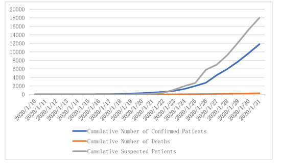
Figure 1. Number of confirmed patients and deaths in the past month.

Table 1. Number of confirmed patients and deaths in the past month.

Date	Cumulative Number of Confirmed Patients	Cumulative Number of Deaths	Cumulative Suspected Patients
10/01/2020	41	1	0
11/01/2020	41	1	0
12/01/2020	41	1	0
13/01/2020-	41	1	0
14/01/2020	41	1	0
15/01/2020	41	2	0
16/01/2020	45	2	0
17/01/2020	62	2	0
18/01/2020	121	3	0
19/01/2020	198	3	0
20/01/2020	291	6	54
21/01/2020	440	9	136
22/01/2020	571	17	393
23/01/2020	830	25	1072
24/01/2020	1287	41	1965
25/01/2020	1975	56	2684
26/01/2020	2744	80	5794
27/01/2020	4515	106	6973
28/01/2020	5974	132	9239
29/01/2020	7711	170	12,167
30/01/2020	9692	213	15,238
31/01/2020	11,791	259	17,988

The disease spread to all provinces, municipalities, and autonomous regions, with Hubei Province seeing the most serious outbreak. Figure 2 shows the number of confirmed patients (purple) and deaths (orange) in China (MedSci n.d.), with most deaths concentrated in Hubei Province.

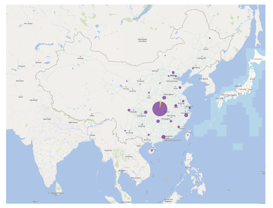
Figure 2. Schematic diagram of the number of infected patients and deaths in China as of 07:30 a.m. on 1 February 2020.

Table 2 shows the number of infections and deaths in each province, municipality, and autonomous region as of 07:30 a.m. on 1 February 2020 (MedSci n.d.), with Hubei Province accounting for 96.23 percent of deaths (204/212) and 59.17 percent of confirmed patients (5806/9812).

Table 2. Number of infected and deceased patients in all provinces, municipalities, and autonomous regions of China as of 07:30 a.m. on 1 February 2020.

Province, Municipality, or Autonomous Region	Number of Confirmed Patients	Number of Deaths
Hubei	5806	204
Zhejiang	538	0
Guangdong	436	0
Henan	352	2
Hunan	332	0
Jiangxi	240	0
Anhui	237	0
Chongqing	211	0
Shandong	184	0
Sichuan	177	1
Jiangsu	168	0
Beijing	139	1
Shanghai	135	1
Fujian	120	0
Guangxi	87	0
Shaanxi	87	0
Yunnan	83	0
Hebei	82	1
Heilongjiang	59	1
Hainan	52	1
Liaoning	48	0
Shanxi	39	0
Tianjin	32	0
Guizhou	29	0
Gansu	29	0
Inner Mongolia	20	0
Ningxia	21	0
Xinjiang	17	0
Jilin	14	0
Hong Kong	12	0
Taiwan	10	0
Qinghai	8	0
Macau	7	0
Tibet	1	0

The outbreak has also spread to other countries, including Thailand, Japan, Singapore, South Korea, Australia, Malaysia, the United States, Germany, France, the United Arab Emirates, Canada, Vietnam, the United Kingdom, Russia, Italy, Nepal, Cambodia, Sri Lanka, Finland, and India (Figure 3). Table 3 shows the number of people infected in each country (MedSci n.d.) as of 07:30 a.m. on 1 February 2020.

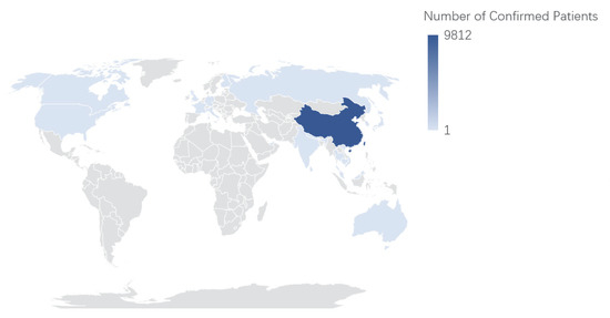
Figure 3. Schematic diagram of the number of infected patients around the world.

Table 3. Number of infected patients around the world as of 07:30 a.m. on 1 February 2020.

Country	Number of Confirmed Patients
China	9812
Thailand	19
Japan	15
Singapore	13
South Korea	11
Australia	9
Malaysia	8
The United States	6
Germany	5
France	5
The United Arab Emirates	4
Canada	3
Vietnam	2
The United Kingdom	2
Russia	2
Italy	2
Nepal	1
Cambodia	1
Sri Lanka	1
Finland	1
India	1

2. Methods and Results

The identification of risk factors is important and can be done by using various methods (He et al. 2019). This study has only predicted the duration, the number of infections and deaths, and the virus’s impact on the economy because the data on COVID-19 are limited. However, these three risk points are highly important. They not only provide useful public health and safety information but also useful insights to economics and policy making. This study used publicly available data from 20 January 2019 to 31 January 2020 to compare COVID-19 with severe acute respiratory syndrome (SARS) and make predictions. The predictions are mainly divided into the following three sections: duration, infections and deaths, and the impact on China’s economy.

2.1. Duration

The predicted duration was mainly based on the curve comparison. Firstly, this study drew the curves of the number of infected, dead, and cured people based on SARS data; then, it found the inflection point (IP) and Key Point (EP) based on the curve and data; finally, it computed the IP and EP of the COVID-19. A schematic diagram of the entire process is shown in Figure 4.

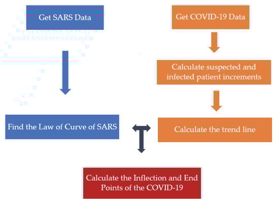
Figure 4. Schematic diagram of the calculation method of the duration of COVID-19 (authors’ figure).

In the first step, this study compared the COVID-19 with SARS data to analyze and predict the time when the virus could continue to infect people. World Health Organization (WHO) data regarding the number of confirmed cases of SARS (2003), deaths, and recoveries are presented in Table 4, with the data on China’s SARS infection from 27 March 2003 to 11 July 2003 shown in Figure 5.

Table 4. Number of confirmed cases of severe acute respiratory syndrome (SARS), deaths, and recoveries in China.

Date	Number of Confirmed Patients	Number of Deaths	Number Recovered
27/03/2003	1179	44	N/A
28/03/2003	1241	44	N/A
29/03/2003	1286	44	N/A
31/03/2003	1346	47	N/A
01/04/2003	1504	50	N/A
02/04/2003	1911	62	N/A
03/04/2003	1938	63	N/A
04/04/2003	1996	62	N/A
05/04/2003	2037	69	N/A
07/04/2003	2172	76	N/A
08/04/2003	2226	78	N/A
09/04/2003	2269	80	N/A
10/04/2003	2307	85	1184
11/04/2003	2389	90	1212
12/04/2003	2440	93	1259
14/04/2003	2631	111	1324
15/04/2003	2673	120	1338
16/04/2003	2727	125	1361
17/04/2003	2781	130	1389
18/04/2003	2899	146	1519
19/04/2003	2899	146	1520
21/04/2003	3390	180	1640
22/04/2003	3464	191	1683
23/04/2003	3800	211	1774
24/04/2003	3947	219	1842
25/04/2003	4152	230	1912
26/04/2003	4329	243	1942
28/04/2003	4537	269	2034
29/04/2003	4941	298	2106
30/04/2003	5128	317	2148
01/05/2003	5328	335	2210
02/05/2003	5511	359	2275
03/05/2003	5693	377	2329
05/05/2003	6034	401	2388
06/05/2003	6172	417	2443
07/05/2003	6340	434	2497
08/05/2003	6491	445	2563
09/05/2003	6622	453	2623
10/05/2003	6731	465	2681
12/05/2003	6881	490	2785
13/05/2003	6983	511	2885
14/05/2003	7061	524	2977
15/05/2003	7131	535	3056
16/05/2003	7172	548	3164
17/05/2003	7194	560	3246
19/05/2003	7295	580	3411
20/05/2003	7350	599	3546
21/05/2003	7387	603	3643
22/05/2003	7478	618	3766
23/05/2003	7549	623	3881
24/05/2003	7573	630	4023
26/05/2003	7629	656	4217
27/05/2003	7648	666	4341
28/05/2003	7665	676	4443
29/05/2003	7718	681	4545
30/05/2003	7732	683	4679
31/05/2003	7744	691	4810
02/06/2003	7759	697	4949
03/06/2003	7756	698	5021
04/06/2003	7756	698	5286
05/06/2003	7755	701	5371
06/06/2003	7756	705	5477
09/06/2003	7762	709	5809
10/06/2003	7769	714	5982
11/06/2003	7771	714	6104
12/06/2003	7772	715	6182
13/06/2003	7781	717	6296
16/06/2003	7780	724	6486
17/06/2003	7779	724	6573
18/06/2003	7779	725	6625
19/06/2003	7777	727	6655
20/06/2003	7777	727	6690
23/06/2003	7774	727	6793
24/06/2003	7769	727	6811
25/06/2003	7769	728	6828
26/06/2003	7765	728	6832
27/06/2003	7764	729	6836
30/06/2003	7761	730	6852
01/07/2003	7761	730	6858
02/07/2003	7759	730	6861
03/07/2003	7757	730	6861
04/07/2003	7757	730	6865
07/07/2003	7757	730	6865
08/07/2003	7754	730	6867
09/07/2003	7754	730	6875
10/07/2003	7757	730	6879
11/07/2003	7754	730	6882

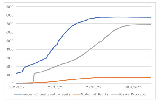
Figure 5. Number of confirmed cases of SARS, deaths, and patients recovered in China.

By following the SARS data, we determined two key time points, one being the Inflection Point (IP). The IP is the time at which the infected person does not worsen significantly. This study argues that when the number of suspected cases increasing per day equals to the number of cases increasing daily, the condition stabilizes and reaches the IP. As per Table 5 and Figure 6, we predicted that the IP would appear on 8 February 2020, based on the Polynomial Method. According to the judgment of Professor Liubo Zhang, Director of the Center for Disinfection and Testing of the Chinese Center for Disease Control and Prevention, combined with media reports, we set the IP of SARS to 14 May 2003 (CCTV 2003; CNTV 2012; Zhejiang News 2017) and its KP (Key Point) to 11 July 2003. We then calculated that the KP of the COVID-19 was 19 February 2020.

Table 5. Increasing daily numbers of infected and suspected patients of COVID-19 throughout January 2020 in China.

Date	Number of Confirmed Patients	Number of Suspected Patients	Case Increases Per Day	Suspected Case Increases Per Day
20/01/2020	291	6	54	N/A
21/01/2020	440	136	149	82
22/01/2020	574	393	134	257
23/01/2020	835	1072	261	679
24/01/2020	1297	1965	462	893
25/01/2020	1985	2684	688	719
26/01/2020	2761	5794	776	3110
27/01/2020	4535	6973	1774	1179
28/01/2020	5997	9239	1462	2266
29/01/2020	7736	12,167	1739	2928
30/01/2020	9720	15,238	1984	3071
31/01/2020	11,821	17,988	2101	2750

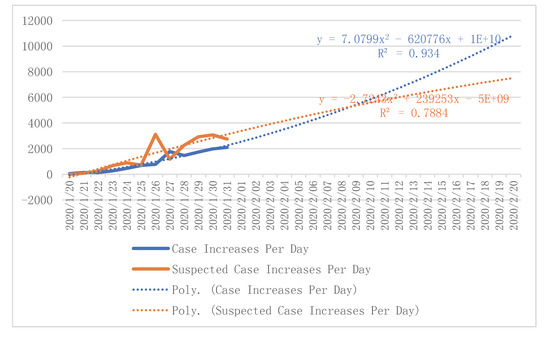
Figure 6. Trend prediction of suspected case increases per day and number of cases increasing per day based on the Excel–Polynomial Method.

IP (COVID-19) = 39 days (31/12/2019–08/02/2020)

IP (SARS) = 194 days (01/11/2002–14/05/2003)

KP (SARS) = 252 days (01/11/2002–11/07/2003)

39/(194/252) = 50.65 days≈50 days (Data lags, fetches one day forward)

KP (COVID-19) = 50 days (2019/12/31–2020/02/19), the Key Point date is 19 February 2020.

Incubation period = 24 days (Wei-jie Guan et al. 2020)

Duration (COVID-19) = 50 + 24 = 74 days (31/12/2019–14/03/2020)

Therefore, our predicted duration was seventy-four days (up to 14 March 2020).

2.2. Infections and Deaths

Previous researchers (e.g., Myers et al. 2000; Ong et al. 2010; Tizzoni et al. 2012) have conducted work to forecast epidemic trends. Two concerns are usually investigated: one relating to geographic development and the other to time series. For the former, if the focus is on accuracy and generalization, the global epidemic and mobility model is popular for urban mobility tracking and forecasting with the prerequisite that transmission tracks of infectors should be timely and fully traced and kept. For example, when SARS occurred in 2003, according to the WHO summary, travel records of super-spreaders, including where they lived, which public transportations they had taken, and who had possibly had contact with them. However, the overwhelmed transportation system and huge population movement during the Chinese New Year holiday increased infectors or carriers of COVID-19 exponentially. That increased the difficulty for us to track all the infectors and carriers’ activities as compared to SARS in 2003. Therefore, we focused on the time series development of the new virus. Time series sequence development contains three components: trend, season, and cycle. The three factors should be considered equivalently. The Autoregressive Moving Average model (ARMA) and Autoregressive Integrated Moving Average model (ARIMA) are widely used to conduct time series analysis and prediction (forecasts) in finance, business, real estate and epidemics. ARIMA is based on ARMA by including integration. If the dataset rejects the stationary hypothesis, this proves that the dataset is stationary and that ARMA is the better choice to perform the prediction. Conversely, if it cannot reject the hypothesis, the dataset is not stationary, and therefore ARIMA should be adopted. The difference should be conducted multiple times on training data in ARIMA to ensure a stationary series for the next step (Li and Chau 2016; Mollison 1977; Riley 2007; Valipour et al. 2013; Nieto et al. 2018). The flowchart is shown in Figure 7.

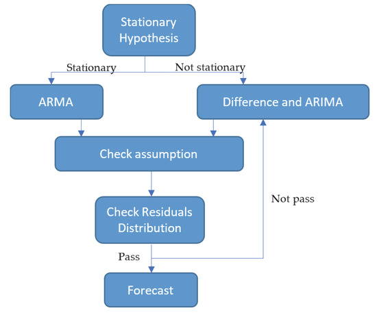
Figure 7. Time series data analysis and prediction (forecasts) process for ARIMA and ARMA

Taking the number of patients as an instance, the P-value is 0.8. It indicates that we can reject the stationary hypothesis. For the analysis, we set

$$X_t=c+ {\displaystyle \sum }_{i=1}^p{\phi }_i X_{t-i}+ {\epsilon }_t, t\in \left\{1, 2, 3\cdots , N\right\}$$

where ${\phi }_1,{\phi }_{2,}\cdots {\phi }_p$ are parameters, $c$ is a constant, and the random variable ${\epsilon }_t$ is the white noise. $X_t$ stands for a time series. N stands for the length of $X_t$.

In this case, we treated the growth of patients, deaths, or suspected cases as a series changing with time. Auto-covariance of the temporal series can be represented by:

$$Co{v}_k=E\left(\left(X_t-\mu \right)\left(X_k-\mu \right)\right)$$

To exempt the effect of scale of different samples, we introduced correlation based on covariance, where correlation is a scale-free measure compared with covariance.

$$Corr\left[X_t, X_k\right]=\frac{Cov\left[X_t, X_k\right]}{\sqrt{V\left[X_t\right]}\sqrt{V\left[X_k\right]}}=\frac{{\sigma }_{12}}{{\sigma }_1{\sigma }_2}, V\left[X\right]={\sigma }^2$$

Since we here compared elements of different time slots from the same time series, and used autocorrelation to measure the effect of previous performance on current data:

$$ACF\left(k\right)={{\displaystyle \sum }}_{t=k+1}^N\frac{\left(Z_t-\overline{Z}\right)\left(Z_k-\overline{Z}\right)}{{{\displaystyle \sum }}_{t=1}^n{\left(Z_t-\overline{Z}\right)}^2}$$

It is defined as describing the relationship between two elements on different time slots based on time intervals to find the pattern with time passing. However, ACF here is the correlation between the t element with the one of k lag. Actually, it is not just about $Z_t$ and $Z_{t-k}$. Because $Z_t$ is also affected by elements between them, e.g. $Z_{t-1}, Z_{t-2}, \cdots , Z_{t-k+1}$. And these elements also have relevance with $Z_t$ and $Z_{t-k}$. So we here introduced partial autocorrelation (PACF). It eliminates the influence of elements between $Z_t$ and $Z_{t-k}$.

We then draw two plots on autocorrelation and partial autocorrelation.

Autocorrelation is shown as per Figure 8:

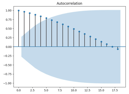
Figure 8. Autocorrelation plot graph for patients’ dataset. k lag is set on x – coordinate and y is set on y. It shows that with time interval larger, the correlation goes down.

Partial autocorrelation is shown in Figure 9:

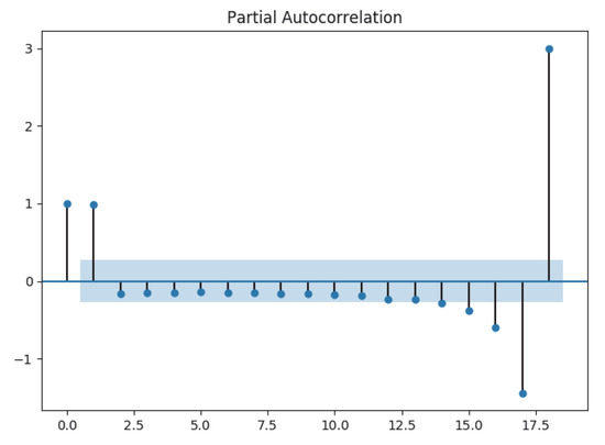
Figure 9. Partial autocorrelation plot graph for the patients’ dataset. The lag between 0.0 to 1.25 and 17.0 towards 18.0 has relevance.

According to these two plots, we know that $p=2$ and $q=2$, and the Akaike information criterion estimator is used to generate $p=2$ and $q=2$ again for verification, which are equal. Alternatively, we may use automatic parameter modification Python library to generate models (Pyramid_Arima), which is shown in Figure 10. Here p stands for the number of lag observations included in the model, also called the lag order, d is the number of times that the raw observations are differenced, also called the degree of differencing. And q is the size of the moving average window.

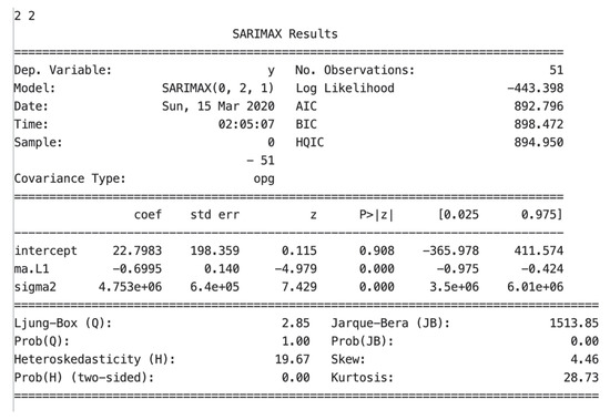
Figure 10. Pyramid_Arima Python lib parameters autocorrection result.

There is no obvious low correlation after k lag either in PACF nor in ACF, so we used ARMA to do the prediction. To clarify, if there was clear correlation performance after k lag in ACF only, we used Moving Average (MA); if only in PACF we used Autoregression (AR). If neither shows correlation, we use ARMA. Under the ARMA condition, if the performance with time passing is stable, we used ARMA; if not stable, we used ARIMA to deal with random unstableness.

Through our calculations, we attained the forecast results for 20 March 2020; simultaneously, we assumed that after March 20, the condition would become stable, and the number would not have major changes. The results are shown in Table 6, Figure 11, Figure 12 and Figure 13.

Table 6. Predicted number of patients and deaths.

Date	Number of Confirmed Patients	Number of Predicted Patients	Number of Confirmed Deaths	Number of Predicted Deaths	Number of Confirmed Suspects	Number of Predicted Suspects
10/1/2020	41	23	1	0	0	0
11/1/2020	41	96	1	2	0	0
12/1/2020	41	94	1	1	0	0
13/1/2020	41	98	1	2	0	0
14/1/2020	41	102	1	2	0	0
15/1/2020	41	105	2	2	0	0
16/1/2020	45	108	2	3	0	0
17/1/2020	62	116	2	3	0	0
18/1/2020	121	139	3	3	0	0
19/1/2020	198	216	3	4	0	0
20/1/2020	291	310	6	4	54	0
21/1/2020	440	420	9	7	136	57
22/1/2020	571	598	17	11	393	181
23/1/2020	830	744	25	21	1072	533
24/1/2020	1287	1051	41	31	1965	1500
25/1/2020	1975	1602	56	52	2684	2720
26/1/2020	2744	2425	80	70	5794	3475
27/1/2020	4515	3313	106	100	6973	7587
28/1/2020	5974	5468	132	130	9239	9176
29/1/2020	7711	7102	170	161	12167	10894
30/1/2020	9692	9045	213	203	15238	14714
31/1/2020	11791	11243	259	250	17988	18210
1/2/2020	14380	13529	304	302	19544	20890
2/2/2020	17205	16397	361	353	21558	21725
3/2/2020	20438	19487	425	415	23214	23302
4/2/2020	24324	23029	490	482	23260	25042
5/2/2020	28018	27327	563	553	24702	24156
6/2/2020	31161	31251	636	633	26359	25366
7/2/2020	34546	34390	722	711	27657	27878
8/2/2020	37198	37845	811	803	28942	29128
9/2/2020	40171	40325	908	896	23589	30212
10/2/2020	42638	43275	1016	1000	21675	21810
11/2/2020	44653	45573	1113	1115	16067	17876
12/2/2020	59804	47334	1367	1219	13435	12438
13/2/2020	63851	66255	1380	1497	10109	9169
14/2/2020	66492	69603	1457	1515	8969	7137
15/2/2020	68500	71332	1665	1627	8228	6623
16/2/2020	70548	72512	1770	1787	7264	7249
17/2/2020	72436	73992	1868	1873	6242	6399
18/2/2020	74185	75435	2004	1983	5248	5229
19/2/2020	74576	76831	2118	2115	4922	4217
20/2/2020	75465	76567	2236	2231	5206	4212
21/2/2020	76288	77148	2345	2358	5365	5138
22/2/2020	76936	77735	2442	2468	4148	5570
23/2/2020	77150	78166	2592	2562	3434	3655
24/2/2020	77658	78097	2663	2708	2824	2426
25/2/2020	78064	78496	2715	2768	2491	2136
26/2/2020	78497	78795	2744	2819	2358	1986
27/2/2020	78824	79161	2788	2815	2308	2095
28/2/2020	79251	79410	2835	2826	1418	2191
29/2/2020	79824	79812	2870	2842	851	961
1/3/2020		80411		2871		87
2/3/2020		81021		2880		0
3/3/2020		81654		2901		0
4/3/2020		82310		2921		0
5/3/2020		82988		2943		0
6/3/2020		83690		2964		0
7/3/2020		84414		2986		0
8/3/2020		85161		3008		0
9/3/2020		85930		3031		0
10/3/2020		86723		3054		0
11/3/2020		87538		3078		0
12/3/2020		88376		3102		0
13/3/2020		89237		3126		0
14/3/2020		90121		3151		0
15/3/2020		91027		3176		0
16/3/2020		91956		3202		0
17/3/2020		92909		3228		0
18/3/2020		93883		3255		0
19/3/2020		94881		3281		0
20/3/2020		95901		3309		0

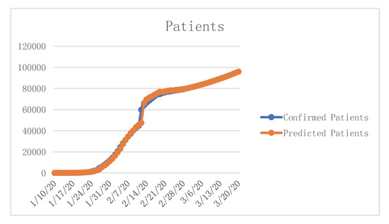
Figure 11. Predicted number of patients.

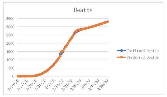
Figure 12. Predicted number of deaths.

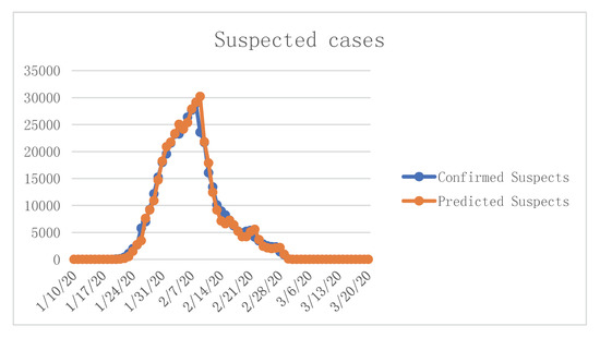
Figure 13. Predicted number of suspects.

Our prediction results show that COVID-19 would be effectively controlled by 19 February 2020, the number of infected patients was expected to be 133,548, the number of deaths was expected to be 1517, and the case fatality rate (CFR) was 1.14 percent. After that, the number of infections and deaths would stabilize at these two values. The condition would gradually stabilize, more and more people would recover, and social production activities should begin to return to normal after 14 March 2020.

2.3. Impact on China’s Economy

Due to the complexity of China’s economic system, this study focused on COVID-19′s impact on workers’ income and the impact on China’s GDP. Individual’s income represents China’s microeconomy while GDP represents its macroeconomy. The impact on work is in the next section, which forecasts GDP.

To achieve these goals, we obtained GDP data for 2000–2019 from the (National Bureau of Statistics n.d.), as shown in Table 7.

Table 7. China’s GDP by Quarter, 2000–2019.

Year and Quarter	GDP (100 Million RMB)	Year and Quarter	GDP (100 Million RMB)	Year and Quarter	GDP (100 Million RMB)	Year and Quarter	GDP (100 Million RMB)
2000Q1	21,329.9	2005Q1	40,453.3	2010Q1	87,501.3	2015Q1	151,137.9
2000Q2	24,043.4	2005Q2	44,793.1	2010Q2	99,347.4	2015Q2	168,549.7
2000Q3	25,712.5	2005Q3	48,047.8	2010Q3	105,963.7	2015Q3	176,597.7
2000Q4	29,194.3	2005Q4	54,024.8	2010Q4	119,306.8	2015Q4	192,572.9
2001Q1	24,086.4	2006Q1	47,078.9	2011Q1	104,469.9	2016Q1	162,410
2001Q2	26,726.6	2006Q2	52,673.3	2011Q2	118,895.9	2016Q2	181,408.2
2001Q3	28,333.3	2006Q3	56,064.7	2011Q3	126,562.2	2016Q3	191,010.6
2001Q4	31,716.8	2006Q4	63,621.6	2011Q4	138,012.1	2016Q4	211,566.2
2002Q1	26,295	2007Q1	57,159.3	2012Q1	117,357.6	2017Q1	181,867.7
2002Q2	29,194.8	2007Q2	64,781.6	2012Q2	131,320.6	2017Q2	201,950.3
2002Q3	31,257.3	2007Q3	69,482.1	2012Q3	138,089.6	2017Q3	212,789.3
2002Q4	34,970.3	2007Q4	78,669.3	2012Q4	151,812	2017Q4	235,428.7
2003Q1	29,825.5	2008Q1	69,373.6	2013Q1	129,449.6	2018Q1	202,035.7
2003Q2	32,537.3	2008Q2	78,711.8	2013Q2	143,518.7	2018Q2	223,962.2
2003Q3	35,291.9	2008Q3	82,460.1	2013Q3	152,222.7	2018Q3	234,474.3
2003Q4	39,767.4	2008Q4	88,699	2013Q4	167,772.3	2018Q4	258,808.9
2004Q1	34,544.6	2009Q1	73,979.2	2014Q1	140,759.8	2019Q1	218,062.8
2004Q2	38,700.8	2009Q2	83,865.8	2014Q2	156,489.6	2019Q2	242,573.8
2004Q3	41,855	2009Q3	89,846.9	2014Q3	165,484.7	2019Q3	252,208.7
2004Q4	46,739.8	2009Q4	100,825.8	2014Q4	180,828.9	2019Q4	278,019.7

Based on data from the National Bureau of Statistics of China, we have a rising trend of GDP for the past 2 decades (Figure 14). The question is that whether the trend keeps pace with the lag in the trade war and COVID-19.

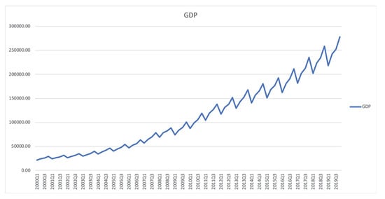
Figure 14. 2000–2019 GDP (in 100 million RMB) of the People’s Republic of China.

Figure 14 indicates that GDP kept rising as the trade war problem worsened in the second quarter of 2019. The increase in GDP reduced, possibly indicating worsening data pointing to the risk of a sharper decline, but soon recovered due to the People’s Bank of China’s (PBOC) efforts to help domestic companies, such as an increase in liquidity. However, in other areas of the world, for example the US, where the Federal Reserve has slashed broad borrowing costs since July, the PBOC has been trying to maintain gradual approaches. This is an effective means of constraining re-inflating debt bubbles.

In December 2019, the novel coronavirus epidemic broke out in the center part of China. This caused a fear of cascading spillovers of supply and demand, regardless of whether they would be peripheral or domestic. Katrina Ell, economist at Moody’s Analytics, has already expressed her gloomy view on China’s GDP with a forecast of 5.4 percent for 2020 (Bloomberg 2020).

Because the SARS outbreak had side effects on China’s economy, we labelled both 2003 and 2020 with the same features for data training (Table 8). Considering SARS affected four quarters (2002Q4, 2003Q1, 2003Q2, and 2003Q3), we forecast COVID-19 to be under control by 14 March, people will still need at least one or two months to restore confidence, so we calculated the figures according to a three quarters model (2019Q4, 2020Q1, and 2020Q2).

Table 8. Epidemic label for GDP data training.

Year and Quarter	Epidemic Label	Year and Quarter	Epidemic Label	Year and Quarter	Epidemic Label	Year and Quarter	Epidemic Label
2000Q1	0	2005Q1	0	2010Q1	0	2015Q1	0
2000Q2	0	2005Q2	0	2010Q2	0	2015Q2	0
2000Q3	0	2005Q3	0	2010Q3	0	2015Q3	0
2000Q4	0	2005Q4	0	2010Q4	0	2015Q4	0
2001Q1	0	2006Q1	0	2011Q1	0	2016Q1	0
2001Q2	0	2006Q2	0	2011Q2	0	2016Q2	0
2001Q3	0	2006Q3	0	2011Q3	0	2016Q3	0
2001Q4	0	2006Q4	0	2011Q4	0	2016Q4	0
2002Q1	0	2007Q1	0	2012Q1	0	2017Q1	0
2002Q2	0	2007Q2	0	2012Q2	0	2017Q2	0
2002Q3	0	2007Q3	0	2012Q3	0	2017Q3	0
2002Q4	1	2007Q4	0	2012Q4	0	2017Q4	0
2003Q1	1	2008Q1	0	2013Q1	0	2018Q1	0
2003Q2	1	2008Q2	0	2013Q2	0	2018Q2	0
2003Q3	1	2008Q3	0	2013Q3	0	2018Q3	0
2003Q4	0	2008Q4	0	2013Q4	0	2018Q4	0
2004Q1	0	2009Q1	0	2014Q1	0	2019Q1	0
2004Q2	0	2009Q2	0	2014Q2	0	2019Q2	0
2004Q3	0	2009Q3	0	2014Q3	0	2019Q3	0
2004Q4	0	2009Q4	0	2014Q4	0	2019Q4	1
						2020Q1	1
						2020Q2	1

After exploring the stationary level, we concluded the statistical parameters shown in Table 9.

Table 9. Hypothesis parameters.

Item	ADF	p-Value	p	q
Raw Data	1.966192	0.998627	3	2
First Difference	−2.021152	0.277377	3	2
Second Difference	−1.472205	0.547214	3	0

GDP prediction is a complicated process as that is affected by many economic variables. Here we do not go deeply into the discussion on how these factors are accounted for when calculating GDP. We will explore the temporal relationships within the data.

Figure 14 shows that there is no clear trend. Normally in the economy or business industries, a cyclic performance is considered. Since we can see that there is a fixed season (seasonal = 4), and the cyclic is used to define an unfixed pattern, we confirm the performance of GDP distribution with no trend and seasonal = 4.

Therefore, we have two possible models:

-

Seasonal Autoregressive Integrated Moving-Average with Exogenous Regressors (SARIMAX)

-

Holt Winter’s Exponential Smoothing (HWES)

SARIMAX is an extension of SARIMA that includes the modeling of exogenous variables. In an economy, there are always exogenous variables that have no relationship within the data but are imported by peripheral effects. Here we treat epidemic and time as considerations of exogenous variables for regression. A summary of the SARIMAX model is shown in Figure 15:

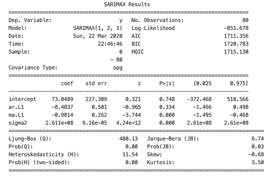
Figure 15. Summary of SARIMAX results.

HWES contains three exponentially weighted linear functions of observations. One works at a prior time step of exponential smoothing. If the dataset contains neither trends nor seasonal trends, single exponential smoothing is used; if it contains trends, then double smoothing is considered; if seasonal with trends are observed, the triple exponential smoothing is used. The model summary is shown in Figure 16:

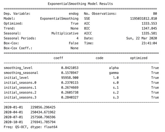
Figure 16. Summary of HWEX.

This study used Python library stats models to explore both of the methods and the prediction of the GDP dataset as listed below, in Table 10 and Figure 17:

Table 10. Predication results.

Year and Quarter	SARIMAX Predicted	HWES Predicted	Expectations
2020Q1	273,611.593	229,856.296	251,733.945
2020Q2	283,894	250,434.672	267,164.336
2020Q3	287,143.419	257,560.797	272,352.108
2020Q4	293,867.856	276,941.786	285,404.821

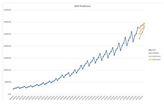
Figure 17. GDP (in 100 million RMB) and the Three Predictions.

In addition, the graph of distribution is below in Figure 17:

3. Analysis of Duration, Number of Infections, and Deaths

Based on the previous analysis, we have summarized the covid-19 and SARS regarding their duration, number of infections, and deaths.

3.1. Duration

We compared the outbreak time and found that there was a high degree of similarity between the two viruses. The duration comparison of the two viruses is shown in Table 11. Regardless of the traditional epidemic model, we conclude that the transfection rate of COVID-19 is 57.87 times faster than that of SARS, as shown in Figure 18.

Table 11. Duration comparison of SARS versus COVID-19.

Virus	Burst Date	End Date	Days	Cumulative Number of Cases in China	Average Number of Cases in China (per Day)
COVID-19	31 December 2019 (Phoenix News n.d.)	14 March 2020 1	75	133,548 2	1780.64
SARS	1 November 2002 (World Health Organization 2002, 2003)	11 July 2003 (World Health Organization 2002, 2003)	252	7754	30.77

¹ Predicted Date; ² Predicted Number.

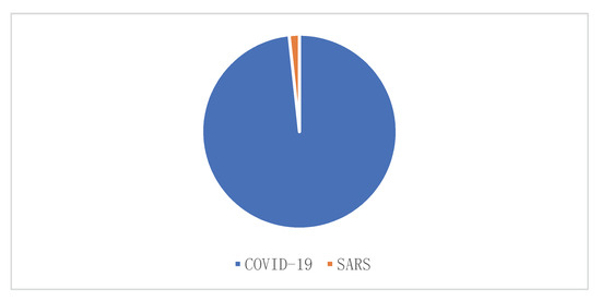
Figure 18. Average number of cases in China (per day).

In 2020, there are 366 days, of which seventy-four will be affected by the COVID-19 virus. In comparison, SARS affected 191 days in 2003, as shown in Figure 19. In terms of duration, the COVID-19 is spreading rapidly, but it will probably not have a longer-lasting impact in China than SARS in 2003.

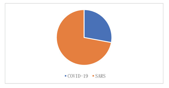
Figure 19. Affected days.

3.2. Infections and Deaths

From 2002 to 2003, SARS also raged in China. According to World Health Organization (2003), the two viruses are highly similar in terms of area and duration of the outbreak, as shown in the comparison in Table 12 and Figure 20.

Table 12. Comparison of SARS versus COVID-19.

Item	COVID-19	SARS	Times
Infections	133,548 1	7754	17.22 2
Deaths	1517 1	730	2.09 2
CFR (%)	1.13	9.42	8.34 3

¹ Predicted Number; ² COVID-19/SARS; ³ SARS/COVID-19.

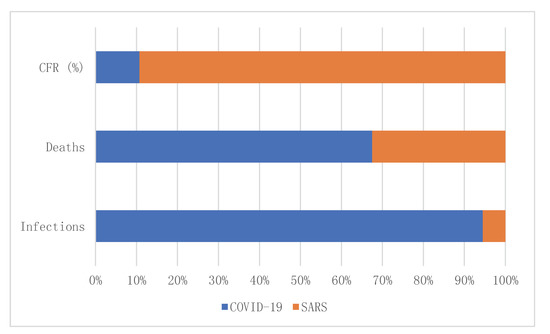
Figure 20. Comparison of SARS versus COVID-19.

As mentioned, most deaths in China (96.23 percent) have been concentrated in Hubei Province. This study consulted the website of the Health Commission of Hubei Province (2020) for information regarding the thirty-two deceased patients in this study time period, which is shown in Table 13.

Table 13. Patient information of the thirty-two deceased persons in Hubei Province.

No.		Sex		Age
1		Female		85
2		Female		69
3		Male		36
4		Male		73
5		Female		70
6		Male		81
7		Female		65
8		Male		70
9		Female		76
10		Male		72
11		Male		79
12		Male		55
13		Male		87
14		Female		66
15		Male		58
16		Male		66
17		Male		78
18		Male		65
19		Male		58
20		Female		67
21		Female		82
22		Male		75
23		Male		66
24		Male		82
25		Female		70
26		Male		53
27		Male		86
28		Male		65
29		Male		84
30		Male		81
31		Female		80
32		Female		82
Average Age of 32 Deceased Patients	Male Ratio (%)	Average Age of 11 Deceased Males	Female Ratio (%)	Average Age of 21 Deceased Females
71.3	34.3	70	65.7	73.8

The CFR of SARS is 8.34 times that of COVID-19. The number of infections and deaths from COVID-19 is 17.22 times and 2.09 times that of SARS, respectively. In terms of CFR, deaths, and infections, many more people have been infected by the new virus in 2019–2020, but the CFR is not high. The average age of the deceased was 71.3 years. The life expectancy of the deceased is 92.2 percent of the life expectancy of Hubei in 2020, 77.3 years (Health Commission of Hubei Province 2017), suggesting that the mortality rate of this disease may not be as alarming as expected.

In addition, except Hubei Province, the CFR in other provinces, municipalities, and autonomous regions is very low (close to 0 in Table 14), and we conjectured the relative high mortality rate in Hubei Province was caused by the following three factors:

Table 14. Comparison of CFR between Hubei and non-Hubei provinces.

CFR (%) of Hubei Province	CFR (%) of Non-Hubei Provinces
3.51	0.20

(1)

The infected people were in fear of this virus. This negatively affected the immune system. In addition, other factors such as tension between doctors and patients and the decline in patient care satisfaction also affected the mood of patients.

(2)

There were too many infected and suspected patients, and many of them were sent to hospitals. On the one hand, as there were insufficient hospital beds, cross-infection occurred.

(3)

There were many elderly people infected in Hubei Province. Many of them also had other underlying conditions and diseases (Health Commission of Hubei Province 2020).

In short, these factors resulted in relatively high mortality rate in Hubei Province.

4. Analysis of Impact on China’s Economy

We analyzed the impact of covid-19 on China’s economy from two aspects: different types of jobs and GDP growth rate.

4.1. Analysis Based on Job Type

Chinese jobs can be divided into four categories according to their occupational characteristics, and we analyzed them separately.

4.1.1. National Staff from Government Departments, Institutions, and State-Owned Enterprises

State departments are established and managed by the state, and wages are coordinated nationwide, so income will not be affected.

4.1.2. Private Enterprise Staff

(1) The adverse impact on private enterprises is relatively more serious. It includes catering, tourism, film, transportation, and other industries. These industries may have been completely closed in recent months.

(2) The income of employees in large and medium-sized private enterprises may be relatively stable because the capital flow of enterprises is usually stable and strong. However, some enterprises’ losses are serious when covid-19 in Europe and the US led to a substantial drop in the demand for goods and services. If covid-19 does not end shortly, these companies may have a liquidity problem..

(3) Small and micro-private companies may be severely damaged and unable to pay salary to their employees. Therefore, this outbreak may lead to bankruptcy or even wind up eventually.

4.1.3. Short-Term and Freelance Staff

Waiters, migrant workers, and live broadcasters are examples of short-term and freelance staff.

(1) Short-term and freelance workers, such as: waiters, migrant workers, may lose their jobs or experience salary reduction. Because jobs such as restaurant waiters cannot work from home, they must stop working during the outbreak.

(2) China is now a hot new market for freelance live broadcasters; the income of these broadcasters is also adversely affected. Their income is usually divided into two parts: the basic salary issued by the contracted company and the gift awarded by the audience (fans). For live broadcasters with fewer fans, the income may not be affected, most of them have not been signed by the platform, and normal live broadcast income is also very small. For live broadcasters with a large number of fans, the income has a greater impact. Because of the advent of the economic winter, the contracting company may face difficulties in cash flow, and because of the loss of income, fans will also reduce or even not give gifts.

4.1.4. Production Staff in Agriculture, Forestry, Animal Husbandry, and Fishery

As a result of the restrictions on their production activities, their income is expected to be affected to some extent, because most of these workers can guarantee self-sufficiency in their basic living.

4.1.5. Summary

In terms of basic living security, the impact may not be that high, but considering that many workers—especially the second, third, and fourth types of workers—may consider raising children or taking out mortgages, car loans, etc. their unstable income will have a rapid impact. In addition, the superior units and bosses of the second and third categories of staff may also cause difficulties for their employees’ lives if they face the problem of capital outages.

The income of national staff will not be affected. In the short term, the income of nonstate workers will drop significantly, the unemployment rate will increase; and the emerging market multinational enterprises cannot achieve improved innovation performance (Mi et al. 2020). However, with the full-scale construction and economic recovery, it is expected that income will gradually stabilize after 14 March 2020.

4.2. GDP

This calculated the economic growth rate of 7.9 percent in 2020, based on the previous forecast results (Table 15). Taking into account factors such as inflation and the real economic growth rate in 2019 (Ning 2020), this study expects the growth rate to be 6.7 percent in 2020. With the compression in recent months, economic development may have a retaliatory rebound.

Table 15. Real economic growth rate in 2020.

Year and Quarter	GDP (100 Million RMB) Per Quarter	GDP (100 Million RMB) Per Year	Economic Growth Rate (%)	Real Economic Growth Rate (%)
2018Q1	202,035.7	919281.1	/	/
2018Q2	223,962.2
2018Q3	234,474.3
2018Q4	258,808.9
2019Q1	218,062.8	990865.0	7.8	6.1
2019Q2	242,573.8
2019Q3	252,208.7
2019Q4	278,019.7
Method		GDP (100 Million RMB) Per Year	Economic Growth Rate (%)	Real Economic Growth Rate (%)
Expectations		1,076,655	8.6	6.7

5. Conclusions

Firstly, by analyzing the environment and situation in China and abroad, this study found that the epidemic is getting worse. Therefore, we obtained official data on infections, deaths, and suspected patients of the COVID-19 virus. Our results showed that the situation in Hubei Province, especially Wuhan City, became very serious. At the same time, the virus has gradually spread to the rest of the world.

Secondly, this study utilised a trend comparison method, ARMA and ARIMA, for data analysis and prediction. Through comparative analysis, we found that the key date of COVID-19 will be obtained on 19 February 2020, and the condition will be fully controlled on 14 March 2020. At the same time, we predicted the number of infections and deaths and the growth of GDP.

Third, this study analyzed the duration of the virus. Although it spreads quickly, it has a much shorter impact than the SARS period, at only seventy-five days. In addition, the number of infected people is estimated to be 133,548, and the death toll is 517. The CFR (%) is significantly lower than SARS.

Finally, this study analyzed the impact of COVID-19 on the economy. Through the analysis of different types of work, it is concluded that private enterprises and their employees, freelancers, as well as agricultural, forestry, animal husbandry, and fishery personnel are more severely affected. These results may be of interest to other countries with COVID-19 infections. Finally, our study predicts that the real GDP growth rate in China in 2020 will be 6.7 percent, which is better than expected.

References

- Bloomberg. 2020. China GDP Forecast Revised to 5.4% in 2020. Available online: https://www.bloomberg.com/news/videos/2020-02-05/our-china-gdp-forecast-revised-to-5-4-in-2020-says-moody-s-analytics-video (accessed on 5 February 2020).
- CCTV. 2003. Special Report on Prevention and Cure of SARS (14 May 2003). Available online: http://fr.cctv.com/lm/560/31/85961.html (accessed on 5 February 2020).
- CNTV. 2012. Heroes of SARS. Available online: http://news.cntv.cn/2012/09/29/ARTI1348893872515797.shtml (accessed on 5 February 2020).
- Guan, Wei-jie, Zheng-yi Ni, Yu Hu, Wen-hua Liang, Chun-quan Ou, Jian-xing He, Lei Liu, Hong Shan, Chun-liang Lei, David S.C. Hui, and et al. 2020. Clinical Characteristics of 2019 Novel Coronavirus Infection in China. medRxiv. [Google Scholar] [CrossRef]
- He, Han, Sicheng Li, Lin Hu, Nelson Duarte, Otilia Manta, and Xiao-Guang Yue. 2019. Risk Factor Identification of Sustainable Guarantee Network Based on Logistic Regression Algorithm. Sustainability 11: 3525. [Google Scholar] [CrossRef]
- Health Commission of Hubei Province. 2017. 13th Five-Year Plan for the Development of Health and Health in Hubei Province. Available online: http://wjw.hubei.gov.cn/bmdt/mtjj/mtgz/201910/t20191030_161998.shtml (accessed on 5 February 2020).
- Health Commission of Hubei Province. 2020. Health Commission of Hubei Province’s Report on Pneumonia of New Coronavirus Infection. Available online: http://wjw.hubei.gov.cn/fbjd/tzgg/ (accessed on 5 February 2020).
- Li, Rita Yi Man, and Kwong Wing Chau. 2016. Econometric Analyses of International Housing Markets. London: Routledge. [Google Scholar]
- Li, Guangdi, and Erik De Clercq. 2020. Therapeutic options for the 2019 novel coronavirus (2019–nCoV). Nature Reviews Drug Discovery. [Google Scholar] [CrossRef] [PubMed]
- Liu, Wei; Xiao-Guang Yue, and Paul B. Tchounwou. 2020. Response to the COVID-19 Epidemic: The Chinese Experience and Implications for Other Countries. International Journal of Environmental Research and Public Health 17: 2304. [Google Scholar] [CrossRef] [PubMed]
- Luo, Yu-Meng, Wei Liu, Xiao-Guang Yue, and Marc A. Rosen. 2020. Sustainable Emergency Management Based on Intelligent Information Processing. Sustainability 12: 1081. [Google Scholar] [CrossRef]
- MedSci. n.d. Real-Time Dynamics of Pneumonia Outbreak of New Coronavirus Infection. Available online: http://m.medsci.cn/wh.do (accessed on 5 February 2020).
- Mi, Lili, Xiao-Guang Yue, Xue-Feng Shao, Yuanfei Kang, and Yulong Liu. 2020. Strategic Asset Seeking and Innovation Performance: The Role of Innovation Capabilities and Host Country Institutions. Journal of Risk and Financial Management 13: 42. [Google Scholar] [CrossRef]
- Mollison, Denis. 1977. Spatial Contact Models for Ecological and Epidemic Spread. Journal of the Royal Statistical Society: Series B (Methodological) 39: 283–313. [Google Scholar] [CrossRef]
- Myers, Monica F., D. J. Rogers, J. Cox, Antoine Flahault, and Simon I. Hay. 2000. Forecasting disease risk for increased epidemic preparedness in public health. Advances in Parasitology 47: 309–30. [Google Scholar] [CrossRef] [PubMed]
- National Bureau of Statistics. n.d. Available online: http://data.stats.gov.cn (accessed on 5 February 2020).
- National Health Commission of the People’s Republic of China. 2020. Outbreak Notification. Available online: http://www.nhc.gov.cn/xcs/yqtb/list_gzbd.shtml (accessed on 5 February 2020).
- Nieto, PJ García, F. Sánchez Lasheras, E. García-Gonzalo, and F. J. de Cos Juez. 2018. PM10 Concentration Forecasting in the Metropolitan Area of Oviedo (Northern Spain) Using Models Based on SVM, MLP, VARMA and ARIMA: A Case Study. Science of the Total Environment 621: 753–61. [Google Scholar] [CrossRef] [PubMed]
- Ning, Jizhe. 2020. Ten Highlights of China’s Economic Operation. Qiushi 3. Available online: http://www.qstheory.cn/dukan/qs/2020-02/01/c_1125497444.htm (accessed on 5 February 2020).
- Ong, Jimmy Boon Som, I. Mark, Cheng Chen, Alex R. Cook, Huey Chyi Lee, Vernon J. Lee, Raymond Tzer Pin Lin, Paul Ananth Tambyah, and Lee Gan Goh. 2010. Real-time epidemic monitoring and forecasting of H1N1-2009 using influenza-like illness from general practice and family doctor clinics in Singapore. PLoS ONE 5: e10036. [Google Scholar] [CrossRef] [PubMed]
- Phoenix News. n.d. Five Consecutive Bird Flu Outbreaks in Hunan, Xinjiang, Major Animal Epidemic Situation Remains Serious. Available online: http://news.ifeng.com/c/7thkaALbJfC (accessed on 5 February 2020).
- Riley, Steven. 2007. Large-Scale Spatial-Transmission Models of Infectious Disease. Science 316: 1298–301. [Google Scholar] [CrossRef] [PubMed]
- Tizzoni, Michele, Paolo Bajardi, Chiara Poletto, José J. Ramasco, Duygu Balcan, Bruno Gonçalves, Nicola Perra, Vittoria Colizza, and Alessandro Vespignani. 2012. Real-time numerical forecast of global epidemic spreading: case study of 2009 A/H1N1pdm. BMC Medicine 10: 165. [Google Scholar] [CrossRef] [PubMed]
- Valipour, Mohammad, Mohammad Ebrahim Banihabib, and Seyyed Mahmood Reza Behbahani. 2013. Comparison of the ARMA, ARIMA, and the Autoregressive Artificial Neural Network Models in Forecasting the Monthly Inflow of Dez Dam Reservoir. Journal of Hydrology 476: 433–41. [Google Scholar] [CrossRef]
- Wang, Chuanyi, Zhe Cheng, Xiao-Guang Yue, and Michael McAleer. 2020. Risk Management of COVID-19 by Universities in China. Journal of Risk and Financial Managment 13: 36. [Google Scholar] [CrossRef]
- World Health Organization. 2002. Summary Table of SARS Cases by Country, 1 November 2002–7 August 2002. Available online: https://www.who.int/csr/sars/country/country2003_08_15.pdf?ua=1 (accessed on 5 February 2020).
- World Health Organization. 2003. SARS: Status of the Outbreak and Lessons for the Immediate Future, WHA 56. May 20. Available online: https://www.who.int/csr/media/sars_wha.pdf?ua=1 (accessed on 5 February 2020).
- Yue, Xiao-Guang, Xue-Feng Shao, Rita Yi Man Li, M. James C. Crabbe, Lili Mi, Siyan Hu, Julien S. Baker, and Gang Liang. 2020. Risk Management Analysis for Novel Coronavirus in Wuhan, China. Journal of Risk Financial Management 13: 22. [Google Scholar] [CrossRef]
- Zhejiang News. 2017. Anti-SARS 14th Anniversary Video Memory: Those Moments We May Have Forgotten. Available online: https://zj.zjol.com.cn/news/675120.html (accessed on 5 February 2020).
© 2020 by the authors. Licensee MDPI, Basel, Switzerland. This article is an open access article distributed under the terms and conditions of the Creative Commons Attribution (CC BY) license (http://creativecommons.org/licenses/by/4.0/).